Learning Environmental Sounds with Multi-scale Convolutional Neural Network

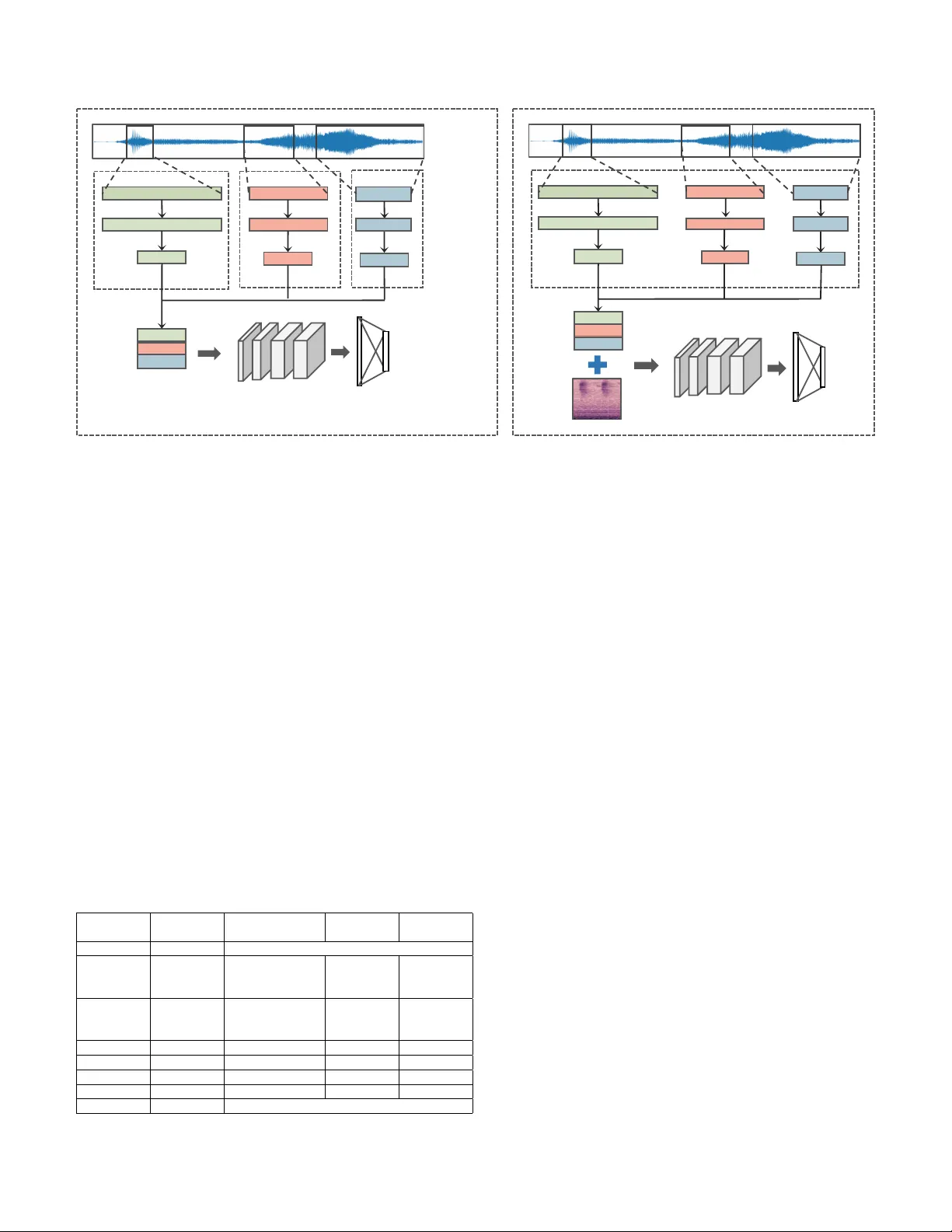
Learning En vironmental Sounds with Multi-scale Con v olutional Neural Network Boqing Zhu 1 , Changjian W ang 1 , Feng Liu 1 , Jin Lei 1 , Zengquan Lu 2 , Y uxing Peng 1 1 Science and T echnology on P arallel and Distributed Labor atory , National University of Defense T echnology 2 Colle ge of Meteor ology and Oceanology , National University of Defense T echnology Changsha, China zhuboqing09@nudt.edu.cn Abstract —Deep learning has dramatically impr oved the perf or - mance of sounds recognition. Howe ver , learning acoustic models directly from the raw wav eform is still challenging. Current wav eform-based models generally use time-domain convolutional layers to extract features. The features extracted by single size filters are insufficient for building discriminativ e repr esentation of audios. In this paper , we propose multi-scale conv olution operation, which can get better audio representation by im- pro ving the frequency resolution and learning filters cross all frequency area. F or lev eraging the wa veform-based features and spectrogram-based features in a single model, we introduce tw o- phase method to fuse the differ ent features. Finally , we propose a novel end-to-end network called W a veMsNet based on the multi-scale conv olution operation and tw o-phase method. On the en vironmental sounds classification datasets ESC-10 and ESC-50, the classification accuracies of our W a veMsNet achieve 93.75% and 79.10% respectively , which improve significantly from the pre vious methods. Index T erms —envir onmenal sounds, multi-scale, con volutional neural networks, features representation I . I N T R O D U C T I O N The environmental sounds are a wide range of everyday au- dio e vents. The problem of en vironmental sound classification (ESC) is crucial for machines to understand surroundings. It is a growing research [1-7] in the multimedia applications. Deep learning has been successfully applied to this task and has generally achieved better results than traditional methods such as random forest ensemble [8] or support v ector machine (SVM) [1]. The majority of models [2, 5] use spectrogram representation as input, such as log-mel features which com- press the amplitude with a log scale on mel-spectrograms. The representations are often transformed further into more compact forms of audio features (e.g. MFCC [4, 6]) depending on the task. All of these processes are designed based on acoustic knowledge or engineering ef forts and features might not suit with the classifier well. Recently increasing focus has extended the end-to-end learning approach down to the le vel of the raw wa veform and features could be learned directly from raw wa veform rather than designed by experts. A commonly used approach is using a time-domain con volution operation on the raw wa veform to extract features as audio representation for classification. Many of them [3, 9, 10] matched or ev en surpassed the performances which employ spectral-based features. Papers [5, 11] have found the complementarity between waveform features and analytic signal transformation (e.g. log-mel). By combining these two kinds of features, they got a notable impro vement on classification accuracy . These works just trained se veral independent models and calculated the av erage of output probabilities of each model. Howe ver , there are still two deficiencies in the existing methods. Firstly , in the previous methods, fixed size filters were employed on the time-series wa veform to extract fea- tures. Ho wev er, it is alw ays a trade-off for choosing the filter size. Wide windows gi ve good frequency resolution, but does not hav e sufficient filters in the high frequency range. Narro w windows can learn more dispersed bands but get lo w frequency resolution [3]. The feature extracted by single size filters might be insufficient for b uilding discriminati ve representation under this dilemma. Secondly , the average method can not make full use of the complementary information in the wa veform features and spectrogram features. It remains to be seen whether it can learn a combination automatically of dif ferent features in a single mode. T o address these two issues, we propose a novel multi- scale con volutional neural network (W a veMsNet), that can extract features by filter banks at multiple different scales and then fuse with the log-mel features in the same model. W e show that our multi-scale CNN outperforms the single-scale models around 3% on classification accuracy with same filters number , which is currently the best-performing method using merely waveform as input. After employing our proposed feature fusion method, the accurac y of classification is further improv ed. In summary , the unique contrib utions of this paper are threefold: 1. W e analyze the inherent deficiencies of single-scale method on features extraction and propose a nov el multi-scale time-domain conv olution operation which can extract more discriminativ e features by improving the frequency resolution and learning filters cross all frequency area. 2. W e propose a method of feature fusion which can combine spectral-based features with wav eform features in a single model. 3. W e design a new multi-scale con volutional neural net- work (W aveMsNet) based on abov e two, composed of filters with dif ferent sizes and strides. It outperforms the single-scale network and achie ves the state-of-the-art model using only waveform as input. The classification accuracy has been further impro ved using our features fusion method. The remainder of this paper is organized as follows. Section 2 discusses related work. Section 3 gives our method and network architecture. Section 4 presents the e xperimental process and results, also, we analyze the results in this section. Finally , Section 5 concludes this paper . I I . R E L ATE D W O R K For years, designing an appropriate feature representation and building a suitable classifier for these features hav e used to be treated as separate problems in the sound classification task [12-17]. F or example, acoustic researchers have been us- ing zero-crossing rate and mel-frequency cepstral coefficients (MFCC) as features to train a random forest ensemble [8] or support vector machine (SVM) [1, 18]. In these methods, clas- sification stage is separated with feature extraction so that the designed features might not be optimal for the classification task. Recently , deep learning based classifiers [19] are used for the ESC task [1]. In particular , Con volutional Neural Network (CNN) has been observed to work better for this problem [5, 19]. Since CNN classifier is useful for capturing the energy modulations across time and frequency-axis of audio spectrograms, it is well suited as classifier for ESC task [19]. The spectral-based features, such as MFCC [4], GTCC [20], and TEO-based GTCC [21] are commonly used as input to extract more abstract features in the ESC task. In [2], Piczak proposed a CNN which once was state-of-the-art method of ESC task using log-mel features and deltas (the first order temporal deriv ati ve) as a 2-channel input. End-to-end learning approach has been successfully used in image classification [22-28] and text domain [29, 30]. In the audio domain, learning from raw audio has been explored mainly in the automatic speech recognition (ASR) task [9-11]. They reported that the performance can be similar to or ev en superior to that of the models using spectral-based features as input. End-to-end learning approach has also been applied to music auto-tagging tasks as well [31]. In [5], T okozume employed an end-to-end system on the ESC task for the first time, but the approach used traditional fixed filter size and stride length. More abundant features would be learned. In the papers [5, 11], learned features can be fix ed with another features at train time. Authors found noticeable im- prov ements by supplementing log-mel filter banks features. They pre-trained two indi vidual models which used ra w wa ve and log-mel as input respectively and calculate the prediction of each window for probability-voting using the a verage of the output of these two networks. W e try to explore an efficient method to combine these two kinds of features in one model in this paper . Further , SoundNet [32] proposed to transfer kno wledge from visual models for sound classification. They used CNN models trained from visual objects and scenes to teach a fea tur e fea tur e fea tur e fea tur e fea tur e multi- scal e pooling and con catena te (a) singl e- sca le feature extra ction (b) multi - scale feature extraction filt ers max pooling mul ti -scale featur e Fig. 1. single-scale vs. multi-scale feature e xtraction feature extractor network for audio. Howe ver , it used a large number of external data, include many video clips. W e hope to find an effecti ve way to learn directly from audio. I I I . M E T H O D S A. Multi-scale con volution operation A popular approach which learns from wa veform is passing the wav eform through a time-domain con volution which has fixed filter size and followed by a pooling step to create in variance to phase shifts and further downsample the signal. This is the so-called single-scale model as Fig. 1(a) sho ws. Howe ver , features extracted by the single-scale model is not discriminativ e enough. First of all, although increasing the time and frequency resolution of the employed representation may be desirable, the uncertainty principle imposes a theoretical limit on how these two can be combined. When analyze a signal in time and frequency together , then more we zoom in into time, the equi valent amount we zoom out in frequency , and vice versa. On the other hand, frequency resolution is more critical for the classification task, if wide windows are employed on the wa veform, we learn more about the low-frequency area, ignoring the high-frequency part, narrow windows beha ve in the opposite way . It is always a trade-off. Single-scale can not always balance them. Therefore, we propose the multi-scale con volution operation (Fig. 1(b)). At multi-scale con volution layer, the wav eform signal w ( i ) are con volved with filters h ( s ) at dif ferent scales s . W e have that x ( s ) j ( n ) = f ( N − 1 X i =0 w ( i ) h ( s ) j ( n − i ) + b ( s ) j ) (1) where f is an acti vation function, N is the length of w ( i ) and b j is an additive bias. Three scales are chosen representati vely ( s = 1 , 2 , 3 ). As thus, to learn high frequency features, filters with a short window are applied at a small stride on the    F ir s t phas e Co n v 1 Co n v 2 Co n v 3 - 6 fc mu l t i - sca l e fea tu r e s output wave f orm fr oz en S ec ond phas e lo g - me l b a cken d netw or k ! " Fig. 2. Network Architectur e and T wo-phases T raining. Architecture of W aveMsNet and two-phases training method for ESC task. wa veforms. Lo w-frequency features, on the contrary , employ a long windo w that can be applied at a larger stride. At the same time, we wish to learn high frequency resolution through the long windo w (actually it does as shown in section IV -D). Then feature maps at different scales are concatenate alone f r eq uency axis and a multi-scale max pooling is employed to downsize the feature map to the same dimension on the time axis. B. F eature Fusion While we considering both the wa veform and analytic signal transformation, one of the mainstream approaches is training sev eral independent models and calculating the average of output probabilities of each model. The improv ement of the classification performance after this simple combination (as shown in section IV -C) indicates that our multi-scale features hav e the capacity to complement the log-mel features. As our experiments reveal later (T able III), simple combi- nation (a veraging the probabilities) does not make full use of T ABLE I T H E L AYE R S C O N FIG U R A T I ON O F W A V E M S N E T . layer name output size filter size, filters number filter stride max pooling Input 66150 - Con v1 I: 66150 II: 13230 III: 6615 I: 11 × 1 , 32 II: 51 × 1 , 32 III: 101 × 1 , 32 I: 1 II: 5 III: 10 no pooling Con v2 441 11 × 1 , 32 1 I: 150 II: 30 III: 15 Con v3 32 × 40 3 × 3 , 64 1 × 1 3 × 11 Con v4 16 × 20 3 × 3 , 128 1 × 1 2 × 2 Con v5 8 × 10 3 × 3 , 256 1 × 1 2 × 2 Con v6 4 × 5 3 × 3 , 256 1 × 1 2 × 2 Fc 4096 4096, dropout: 50% the information in dif ferent features and the performance is not optimal. W e explore the learning method to extract the complementary information between the different features in a single end-to-end model. W e propose a two-phase method of feature fusion, which aims at joining log-mel features in. In the first phase, a feature extractor will be trained and the multi-scale feature map X ∈ R H × W will be e xtracted directly on the time-series wa veforms, where H and W is the f r eqency and time di- mension respecti vely . In the second phase, the same-dimension log-mel features Y ∈ R H × W are stack on the wav eform features to form a two-channels feature map. It is conv olved with learnable kernels and put through the acti vation function f to form the output feature map O j ∈ R H × W O j = f ( X i ∈ M X i ∗ k ij + X i ∈ L Y i ∗ k ij + b j ) (2) where M and L represent selections of the multi-scale feature map and log-mel feature map respecti vely , the j th output map is produced by k ernel k ij and each output map is given an additiv e bias b. Then we fine-tune the backend network while keeping the parameters in the feature extractor fixed during the back propagation. T o overcome the vanishing gradient problem, we designed a shallow backend network. Deeper networks can extract more abstract features, b ut with the deepening of the network layer, small gradients ha ve little effect on the weights in front of the network, e ven if residual connection is used (as e xperiment in section IV -C). By reducing the number of backend network layers, the first fe w layers could ha ve a good ability to extract discrepant features and as con vergent as possible. C. Neural Network Arc hitecture According to the above, we propose the multi-scale con vo- lutional neural network with feature fusion as Fig. 2 sho ws. Firstly , we apply the multi-scale con volution operation on the input wav eform. Three scales are chosen: I: (size 11, stride 1), II: (size 51, stride 5), III: (size 101, stride 10). Each scale has 32 filters in the first layer . Another con volutional layer is followed to create in v ariance to phase shifts with filter size 11 and stride 1. W e aggressi vely reduce the temporal resolution to 441 with a max pooling layer to each scale feature map. W e use non-overlapping (the pooling stride is same as pooling size) max-pooling. Then, we concatenate three feature map together and we get the multi-scale feature map as sho wn in Fig. 2. Then, the backend network is applied on the multi-scale fea- ture map which can be seen as time-frequency representation. Four con volutional layers are followed. W e use small receptiv e field 3 × 3 in f req uency × time for all layers. Small filter size reduces the number of parameters in each layer and control the model sizes and computation cost. W e apply non-overlapping max pooling after con volutional layers. Finally , we apply a fully connected layers with 4096 neurons and an output layer which has as many neurons as the number of classes. W e adopt auxiliary layers called batch normalization (BN) [33] after each con volutional layer (before pooling layer). BN alleviates the problem of exploding and vanishing gradients, a common problem in optimizing deep architectures. It nor- malizes the output in one batch of the pre vious layer so the gradients are well beha ved. W ith BN layer applied, we can accelerate the training phase. D. Implementation Details W e use the exactly same model in two training phases. When training, we randomly select a 1.5 seconds w aveform as input which were employed by T okozume [5], in testing phase, we use the probability-voting strategy . Rectified Linear Units (ReLUs) ha ve been applied for each layer . W e use momentum stochastic gradient descent (momentum SGD) optimizer to train the network where momentum set as 0.9. W e run each model for 180 epochs until conv ergence. Learning rate is set as 10 − 2 for first 50 epochs, 10 − 3 for next 50 epochs, 10 − 4 for next 50 epochs and 10 − 5 for last 30 epochs. The weights in each model are initialized from scratch without an y pre- trained model or Gammatone initialization because we want to learn the complements feature with handcraft features such as mel-scale feature. Dropout layers are followed full connected layer with a dropout rate of 0.5 to avoid ov erfitting. All weight parameters are subjected to ` 2 regularization with coefficient 5 × 10 − 4 . I V . E X P E R I M E N T S A. Datasets ESC-50 and ESC-10 datasets which are public labeled sets of en vironmental recordings are used in our e xperiments. ESC- 50 dataset comprises 50 equally balanced classes, each clip is about 5 seconds and sampled at 44.1kHz. The 50 classes can be di vided into 5 major groups: animals, natural soundscapes and w ater sounds, human non-speech sound, interior/domestic sounds, and exterior/urban noises. The dataset provides an exposure to a variety of sound sources, some very common ( laughter , cat meowing, do g barking ), some quite distinct ( glass br eaking, brushing teeth ) and then some where the differences are more nuanced ( helicopter and airplane noise ). The ESC-10 is a selection of 10 classes from the ESC- 50 dataset. Datasets have been prearranged into 5 folds for comparable cross-v alidation and other experiments [2, 5, 32] used these folds. For a fair comparison, the same folds division are proposed in our ev aluation. The audios are not down- sampled, because we want to keep more high frequency information. W e shuffle the training data b ut do not perform any data augmentation. B. Effectiveness of multi-scale convolution operation W e hypothesize that applying multi-scale con volution op- eration could allow each scale to learn filters selective to the frequencies that it can most efficiently represent. T o test our hypothesis, we train variant models in single scales. W e compare the performance with constant filter size at three different scales, small receptiv e field model (SRF), middle receptiv e field model (MRF), and lar ge receptiv e field model (LRF). These three models remain only one corresponding scale (SRF remains scale I, MRF remains scale II and LRF remains scale III) and use triple filters in Con v1 and Con v2 layers for fair comparison with multi-scale. These three v ariant models are trained separately . The input and the rest of network is same as Fig. 2 T able II shows the accuracies using multi-scale features and single-scale features when we only take wav eform as input. Experiments conduct with different filter sizes, strides and pooling size in the CNN training. W e observe that our W aveMsNet substantially improve the performance (88.05% and 70.05%). W e hav e an improvement of 2.95%, 2.50%, 3.00% compared with SRF , MRF , and LRF model respectively with same filters number on ESC-50 dataset. Also, multi-scale model achieves at lest 1.35% improvement on ESC-10. T o our knowledge, it is the best-performing end-to-end model which only use wa veform as input. The significantly improv ement from single-scale to multi-scale proves that dif ferent scales hav e learned more discriminativ e features from raw wav eform. Further , the improvement is more notable on the lar ger dataset (ESC-50), which implies that our model has good generaliza- tion ability . T o further verify the ef fectiv eness of the multi-scale con vo- lution operation, we employ different backend networks, all T ABLE II C O MPA R IS O N O F T H E M U L T I - SC A L E A N D S I N GL E - S CA L E M O D EL Model Filter numbers Mean accuracy(%) Scale I Scale II Scale III ESC-10 ESC-50 SRF 96 0 0 85.85 67.10 MRF 0 96 0 86.70 67.55 LRF 0 0 96 85.75 67.05 W a veMsNet 32 32 32 88.05 70.05 50 53 56 59 62 65 68 71 Ale xNe t VG G11_bn ResNe t50 W ave MsNe t Me a n Acc ur ac y (%) SRF MRF LRF Mult i - sca l e Fig. 3. Effectiveness of multi-scale models. T o further v erify the ef- fectiv eness of the multi-scale. W e compare W a veMsNet and other three backend networks: AlexNet, VGG, ResNet. On ESC-50, Multi-scale models are superior to single-scale ones re gardless of the backend networks. of which are widely used and well-preformed in the field of image. They are AlexNet [22], VGG (11 layers with BN) [23] and ResNet (50-layers) [24]. As Fig. 3 demonstrates, the multi-scale models consistently outperform single-scale models. It indicates that multi-scale models have a wide range of effecti veness. In our shallow network, v anishing gradient problem is well suppressed during back-propagating. The first two layers of our network can con ver ge better so that our W a veMsNet matches or e ven exceeds other very deep con volutional neural network. C. T wo-phase feature fusion W e train our backend network with the log-mel features to form a new network and simply combine it with W a veMsNet we got abov e – calculating the average of output probabilities of each model. As sho wn in T able III, we get 89.50% and 78.50% accuracy on ESC-10 and ESC-50. The improvement on accuracy indicates that the multi-scale features we hav e extracted from wav eforms are highly complementary from log- mel features. Now , we use the two-phase method to fuse the features. In first phase, we only use waveform as input to train W a veM- sNet. In second phase, we fuse log-mel features with the multi- scale features as we introduced in section III-B. W e fine-tune the layers after Con v3 and keep the front part of the network (Con v1 and Con v2) freezing. That is to say , in the second training phase, parameters will only update in layers after Con v3 and not update in Con v1 and Conv2. T able III shows results after the second phase and compares the performance when the Conv1 and Conv2 are frozen and T ABLE III P E RF O R M AN C E S W IT H D I FF E RE N T T R A IN I N G M E TH O D S Method Accuracy (%) ± std ESC-10 ESC-50 after first phase 88.05 ± 2.50 70.05 ± 0.63 simple combination(two models) 89.50 ± 1.23 78.50 ± 1.50 after second phase (not frozen) 92.50 ± 1.87 77.85 ± 2.10 after second phase(frozen) 93.75 ± 0.63 79.10 ± 1.63 one-phase training method 88.75 ± 2.12 76.35 ± 1.25 T ABLE IV C O MPA R IS O N O F A C C U R AC Y O F E S C D AT A S E T Model Mean accuracy(%) ESC-10 ESC-50 Piczaks CNN [2] 81.00 64.50 T okozumes Logmel-CNN [5] - 66.50 En vNet [5] - 64.00 D-CNN-ESC [7] - 68.10 AlexNet [6] 85.00 69.00 GoogLeNet [6] 90.00 73.20 A ytar [32] 92.20 74.20 En vNet ⊕ Logmel-CNN [5] * - 71.00 W a veMsNet after first phase(ours) 88.05 70.05 W a veMsNet after second phase(ours) 93.75 79.10 Human performance [1] 95.70 81.30 * The ⊕ sign indicates system simple combination before softmax not frozen. The accuracies ha ve been greatly improv ed 5.70% and 9.05% on ESC-10 and ESC-50 datasets after second phase. In comparison, the improvement is 4.45% and 7.85% on these two datasets when we keep the parameters in Con v1 and Con v2 updatable. The improvements are more ob vious at second phase if we freeze the parameters than not. W e infer that its because log-mel features will disturb the networks front part which aiming at e xtracting features from w aveform. Furthermore, we compare with one-phase training method which fuse the multi-scale features with log-mel features from the beginning. The performances degrade 5.00% and 2.75% respectiv ely because the layers would be optimized under dif- ferent hyper-parameters. The network would hard to take into account the wav eform and log-mel if we unify the two training phase into one. The two-phase method combines wa veform- based features with spectral-based features in a single model instead of training two separate models as pre vious works did and outperforms others. D. Results and Analysis Our proposed work is compared with the other studies in literature in T able IV. W aveMsNet trained after two phase get an accuracy of 93.75% and 79.10% on ESC-10 and ESC-50 which about to match the performance of untrained human participants on this datasets (95.70% and 81.3%). Fig. 4 shows the responses of the multi-scale feature maps. Most of the filters learn to be band-pass filters. Scale I has learned more dispersed bands across the frequency that can extract feature from all frequency and the trend of the center frequency matches the mel-scale (how human percei ve the sound). But the frequency resolution is lower . On the contrary , scale III has learned high frequenc y resolution bands and most of them locate at the low frequency area. But it does not hav e sufficient filters in the high frequency range. Scale II behav es between scale I and III. This indicts that different scales could learn discrepant features and the filter banks split responsibilities based on what they ef ficiently can represent. This explains why multi-scale models get a better performance than single-scale models shown in T able II. 0 10 20 30 Filter index (sorted) 0 5 10 15 20 Frequency [kHz] 0 10 20 30 Filter index (sorted) 0 5 10 15 20 0 10 20 30 Filter index (sorted) 0 5 10 15 20 Fig. 4. Frequency response of the multi-scale featur e maps. Left shows the frequency response of feature map product by scale I. Middle corresponds to scale II. Right corresponds to scale III. V . C O N C L U S I O N In this paper , we proposed a multi-scale CNN (W a veMsNet) that operates directly on raw wa veform inputs. W e presented our model to learn more efficient representations by multiple scales. It achiev es the state-of-the-art model using only ra w wa veform as input. By the two-phase training method, we fused the waveform and log-mel features in a single model and got a significant improvement in classification accurac y on ESC-10 and ESC-50 datasets. Furthermore, we analyzed the discrimination of features learning at different scales and had insight into the reasons of performance improv ement. A C K N O W L E D G M E N T This work is supported by the National Key Research and Dev elopment Program of China (2016YFB1000100). R E F E R E N C E S [1] K. J. Piczak, “ESC: Dataset for En vironmental Sound Classification, ” in Pr oceedings of the 23rd Annual A CM Conference on Multimedia . A CM Press, pp. 1015–1018. [Online]. A v ailable: http://dl.acm.org/ citation.cfm?doid=2733373.2806390 [2] ——, “En vironmental sound classification with conv olutional neural networks, ” in Machine Learning for Signal Processing (MLSP), 2015 IEEE 25th International W orkshop on . IEEE, 2015, pp. 1–6. [3] W . Dai, C. Dai, S. Qu, J. Li, and S. Das, “V ery deep conv olutional neural networks for raw wa veforms, ” in Acoustics, Speech and Signal Pr ocessing (ICASSP), 2017 IEEE International Confer ence on . IEEE, 2017, pp. 421–425. [4] J. Salamon, C. Jacoby , and J. P . Bello, “ A dataset and taxonomy for urban sound research, ” in ACM International Confer ence on Multimedia , 2014, pp. 1041–1044. [5] Y . T okozume and T . Harada, “Learning environmental sounds with end- to-end con volutional neural network, ” in IEEE International Conference on Acoustics, Speec h and Signal Processing , 2017, pp. 2721–2725. [6] V . Boddapati, A. Petef, J. Rasmusson, and L. Lundberg, “Classifying en vironmental sounds using image recognition networks, ” Pr ocedia Computer Science , v ol. 112, pp. 2048–2056, 2017. [7] X. Zhang, Y . Zou, and W . Shi, “Dilated con volution neural network with leak yrelu for environmental sound classification, ” in International Confer ence on Digital Signal Pr ocessing , 2017, pp. 1–5. [8] A. Liaw , M. Wiener et al. , “Classification and regression by randomfor- est, ” R news , v ol. 2, no. 3, pp. 18–22, 2002. [9] T . N. Sainath, O. V inyals, A. Senior, and H. Sak, “Con volutional, long short-term memory , fully connected deep neural networks, ” in IEEE International Confer ence on Acoustics, Speech and Signal Processing , 2015, pp. 4580–4584. [10] R. Zazo, T . N. Sainath, G. Simko, and C. Parada, “Feature learning with raw-wa veform cldnns for voice activity detection, ” in INTERSPEECH , 2016, pp. 3668–3672. [11] A. S. K. W . W . T . N. Sainath, R. J. W eiss and O. V inyals, “Learning the speech front-end with raw wa veform cldnns, ” in Sixteenth Annual Confer ence of the Internatianal Speec h Communication Association , 2015. [12] D. Barchiesi, D. Giannoulis, S. Dan, and M. D. Plumbley , “ Acoustic scene classification: Classifying en vironments from the sounds they produce, ” IEEE Signal Pr ocessing Magazine , vol. 32, no. 3, pp. 16– 34, 2015. [13] J. T . David Li and D. T oub, “ Auditory scene classification using machine learning techniques, ” AASP Challenge , 2013. [14] A. Rakotomamonjy and G. Gasso, “Histogram of gradients of time- frequency representations for audio scene classification, ” IEEE/ACM T ransactions on Audio Speech & Langua ge Pr ocessing , v ol. 23, no. 1, pp. 142–153, 2015. [15] S. Dan, D. Giannoulis, E. Benetos, M. Lagrange, and M. D. Plumbley , “Detection and classification of acoustic scenes and events, ” IEEE T ransactions on Multimedia , v ol. 17, no. 10, pp. 1733–1746, 2015. [16] G. Roma, W . Nogueira, and P . Herrera, “Recurrence quantification analysis features for environmental sound recognition, ” Annals of the Rheumatic Diseases , v ol. 51, no. 9, pp. 1056–62, 2013. [17] J. Salamon and J. P . Bello, “Unsupervised feature learning for urban sound classification, ” in IEEE International Conference on Acoustics, Speech and Signal Pr ocessing , 2015, pp. 171–175. [18] W . M. Campbell, D. E. Sturim, and D. A. Reynolds, “Support vector machines using gmm supervectors for speaker verification, ” IEEE signal pr ocessing letter s , v ol. 13, no. 5, pp. 308–311, 2006. [19] J. Salamon and J. Bello, “Deep con volutional neural networks and data augmentation for environmental sound classification, ” IEEE Signal Pr ocessing Letter s , v ol. PP , no. 99, pp. 1–1, 2016. [20] M. V acher , J.-F . Serignat, and S. Chaillol, “Sound classification in a smart room en vironment: an approach using gmm and hmm methods, ” in The 4th IEEE Conference on Speech T ec hnology and Human-Computer Dialogue (SpeD 2007), Publishing House of the Romanian Academy (Buchar est) , vol. 1, 2007, pp. 135–146. [21] D. M. Agra wal, H. B. Sailor , M. H. Soni, and H. A. Patil, “Novel teo- based gammatone features for environmental sound classification, ” in Eur opean Signal Pr ocessing Conference , 2017, pp. 1809–1813. [22] A. Krizhevsky , I. Sutske ver , and G. E. Hinton, “Imagenet classification with deep con volutional neural netw orks, ” in International Confer ence on Neural Information Pr ocessing Systems , 2012, pp. 1097–1105. [23] K. Simonyan and A. Zisserman, “V ery deep conv olutional networks for large-scale image recognition, ” arXiv pr eprint arXiv:1409.1556 , 2014. [24] K. He, X. Zhang, S. Ren, and J. Sun, “Deep residual learning for image recognition, ” in Computer V ision and P attern Recognition , 2016, pp. 770–778. [25] G. Huang, Z. Liu, K. Q. W einberger , and L. van der Maaten, “Densely connected con volutional networks, ” in Pr oceedings of the IEEE confer- ence on computer vision and pattern reco gnition , vol. 1, no. 2, 2017, p. 3. [26] O. Ronneberger , P . Fischer, and T . Brox, U-Net: Convolutional Networks for Biomedical Image Se gmentation . Springer International Publishing, 2015. [27] P . Zhang, X. Niu, Y . Dou, and F . Xia, “ Airport detection on optical satel- lite images using deep conv olutional neural networks, ” IEEE Geoscience and Remote Sensing Letters , vol. 14, no. 8, pp. 1183–1187, 2017. [28] Q. W ang, Y . Dou, X. Liu, F . Xia, Q. Lv , and K. Y ang, “Local kernel alignment based multi-view clustering using extreme learning machine, ” Neur ocomputing , v ol. 275, pp. 1099–1111, 2018. [29] X. Zhang, J. Zhao, and Y . LeCun, “Character-lev el conv olutional networks for text classification, ” in Advances in neural information pr ocessing systems , 2015, pp. 649–657. [30] Y . Kim, Y . Jernite, D. Sontag, and A. M. Rush, “Character-aware neural language models, ” Computer Science , 2015. [31] J. Lee, J. Park, K. L. Kim, and J. Nam, “Sample-level deep conv olutional neural networks for music auto-tagging using raw waveforms, ” arXiv pr eprint arXiv:1703.01789 , 2017. [32] Y . A ytar, C. V ondrick, and A. T orralba, “Soundnet: Learning sound rep- resentations from unlabeled video, ” in Advances in Neural Information Pr ocessing Systems , 2016, pp. 892–900. [33] S. Ioffe and C. Szegedy , “Batch normalization: Accelerating deep network training by reducing internal covariate shift, ” in International confer ence on machine learning , 2015, pp. 448–456.