Automatic Music Accompanist

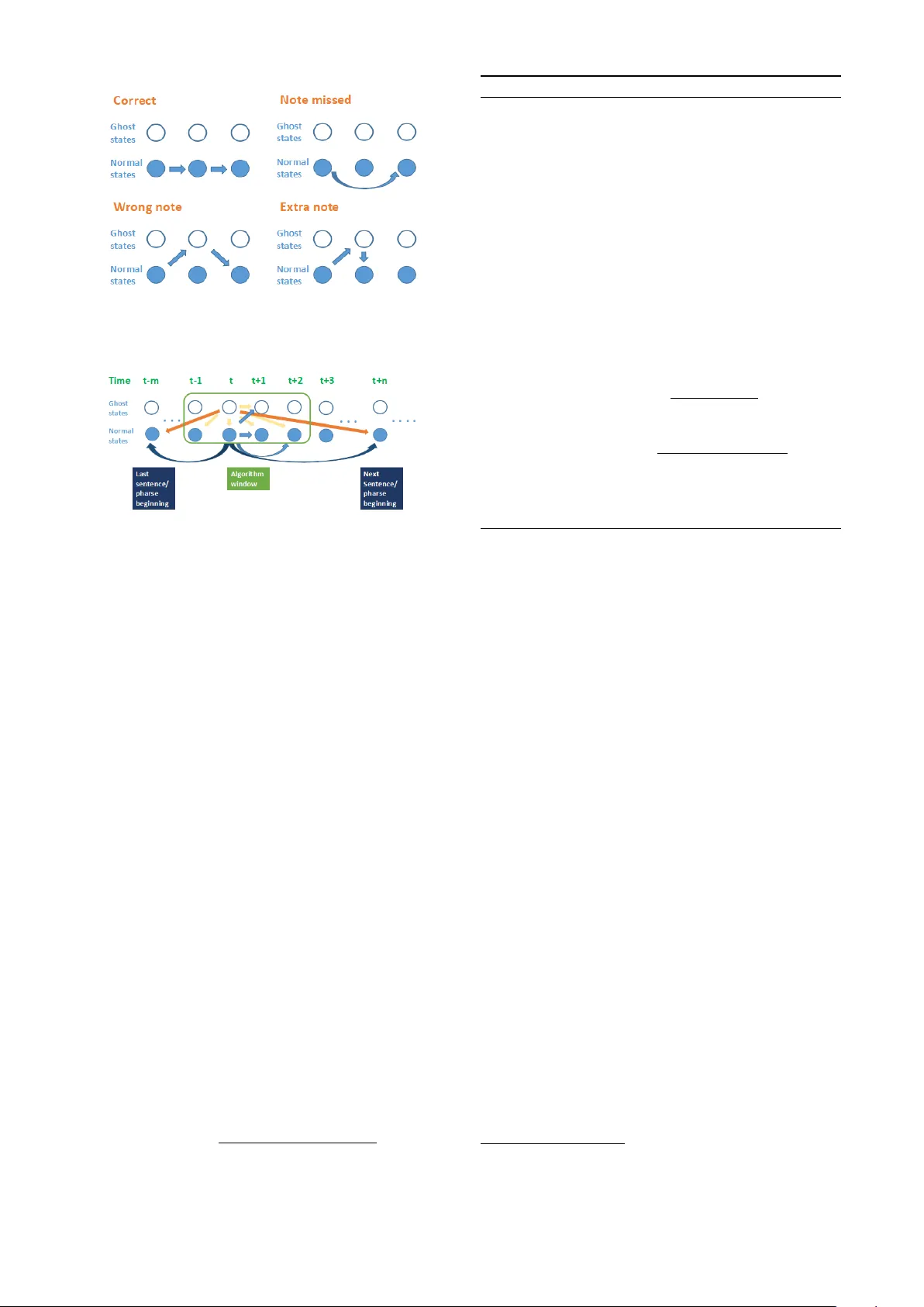
A utomatic Music Accompanist Anyi Rao Nanjing Univ ersity anyirao@smail.nju.edu.cn Francis Lau The Univ ersity of Hong K ong fcmlau@cs.hku.hk ABSTRA CT Automatic musical accompaniment is where a human mu- sician is accompanied by a computer musician. The com- puter musician is able to produce musical accompaniment that relates musically to the human performance. The ac- companiment should follow the performance using obser- vations of the notes the y are playing. This paper describes a complete and detailed construc- tion of a score following and accompanying system using Hidden Markov Models (HMMs). It details how to train a score HMM, how to deal with polyphonic input, how this HMM work when follo wing score, ho w to b uild up a musi- cal accompanist. It proposes a ne w parallel hidden Marko v model for score follo wing and a f ast decoding algorithm to deal with performance errors. 1. INTR ODUCTION Accompanists may not always be av ailable when needed, or av ailable accompanists may not hav e sufficient techni- cal ability to provide adequate accompaniment. A solu- tion for many musicians is to make use of recorded or computer-generated accompaniment where the accompa- niment is static, i.e. nev er changing from one performance to another . This forces the musician to adapt their playing to synchronize with the accompaniment. It is more natural for the musician, though, if the accompaniment adapts to the performer, particularly as a musicians playing tends to be ’free’. T o dynamically synchronize the accompaniment with the performance by the musician, the accompanist should track the performers progress through the score of the piece as they play . Score following is the process whereby a musi- cian follo ws another musicians playing of a musical piece, by tracking their progress through the score of that piece. The term is most commonly used in the context of computer - generated accompaniment, where one or more of the mu- sicians in volv ed are artificial rather than human. The pur- pose of the research outlined in this paper is to construct a automatic accompaniment. In liv e performance, score follo wing must be on-line real- time, i.e. producing accompaniment in time with the soloists playing. This places extra challenges for the score fol- lower . The system has a more limited amount of informa- tion available for analysis: only the notes that hav e been played so far , as opposed to having the whole performance Copyright: c  2017 Anyi Rao et al. to analyse. It requires fast computation speed. The ac- companist needs finish one accompaniment before the next note comes. Our contributions are as follo ws, 1 Our work is the first free open-source W indows based automatic music follo wer and accompanist to our best knowledge. 2 W e construct a comprehensiv e system and show ho w it works with detailed theoretical induction, includ- ing score follo wer training/decoding and score ac- companist. 3 W e propose a fast decoding algorithm, reduced com- putational complexity from O ( n 2 ) do wn to O ( n ) . It is able to work in real time with practical length scores. 4 W e build up two hands parallel HMM to improve accuracy and computational speed. Background There are se veral reasons why a musician may not perform the piece e xactly as written. Changes may be added by mistake: 1. A wrong note is played; 2. Extra notes are added; 3. Scored notes are missed out; 4. The musician loses their place in the music or starts playing from the wrong point in the score. 5. The tempo speeds up or slo ws down unintentionally . Also changes may be added deliber- ately , as the musician adds their own interpretations to the music: 1. The musician adds embellishments such as trills, to decorate the notes; 2. The tempo speeds up or slo ws down deliberately , for musical effect; 3. The piece being played may ha ve rubato or free/impro vised sections, where the musician is free to v ary the tempo and notes played ac- cording to their own choice. T erms Performance: In the conte xt of this project, a performance is defined specifically as the situation where a solo mu- sician (soloist), such as a flute player or singer , performs a piece of music. The solo musician would be accompa- nied by another musician (accompanist) on an instrument such as piano. This may be in a concert or similar sce- nario, performing to an audience, but this condition is not mandatory . What is important is that the soloist is mak- ing an attempt to play through the piece in a linear fashion, from start to finish. Performer/Soloist: The solo musician who is performing the piece; what they play is the most important part of the performance for any audience that may be listening. Accompanist: The musician who is playing the accom- paniment; supporting the soloists performance. Melody/Solo melody: The music that is being played by the soloist. Accompaniment: The music which is played by an ac- companist, during the performance of the soloist. Accom- paniment can be thought of background music which is de- signed to enhance what the soloist is playing and support the soloists performance. Score follower: A computer accompanist that follows the solo melody through the score as it is being played, to produce accompaniment relative to where the soloist is in the score. 2. HIDDEN MARK O V MODELS A musical score is di vided up into a sequence of musical ev ents. (for example one note or one beat can be consid- ered as one modellable musical ev ent) The score follower uses a Hidden Markov Model to rep- resent these musical ev ents, and uses a decoding algorithm to estimate what state the performer is most likely to be in at that time, i.e. which musical event in the score the performer is currently playing. 2.1 HMM Structure W e define the observation states as 12 notes in the western musical chromatic scale. W e ignores octave dif ferences be- tween notes and merely consider 12 possible observ ations: { C, C ] , D, E b , E, F , F ] , G, G ] , A, Bb, B } , as sho wn in Figure 1. The hidden states base on beat and encode the information relates to the beat as detailed in the below sec- tion 2.1.1. The paraments λ of the HMM contains three parts { π , A, B } denoted below . Figure 1. Hidden Marko v Model structure. • N: the number of possible states. W e use N symbols S 1 , S 2 , · · · , S N to denote them. • M: the number of possible observ ations. • π : the prior (initial) state distribution. π = ( π 1 , π 2 , · · · , π N ) and π i = Pr( Q 1 = S i ). • A: the state transition matrix. A ij = P r ( Q t = S j | Q t − 1 = S i ) is the probability of the ne xt state being S j if the current one is S i , 1 ≤ i, j ≤ N. Note that A does not change when t changes. • B: the observation probability matrix. Instead of denoting one probability as B j k , we use b j ( k ) = P r ( O t = V k | Q t = S j ) to denote the probability of the observation being V k when the state is S j , 1 ≤ j ≤ N, 1 ≤ k ≤ M. And, B does not change when t changes. 2.1.1 beat-based r epr esentation If there is a simple tune for which each note is of the same length, the naiv e choice is to model each note as an indi- vidual HMM state. But when music pieces become more complex, it is no longer realistic to model each note as a ne w state, and in- stead the more pertinent aspect to model as a state is each beat, or a fraction of each beat. For such cases, it was necessary to consider how the timing information within the score should be modelled (in addition to ho w the notes should be modelled). The two obvious ways to model a note that is held for longer than one state (i.e. notes that extend ov er a beat or more) are: 1. Allo w states with self-transitions, so the HMM stays in a given state while a note is being held and only mov es out of that state when the note is released. 2. Ha ve a finite number of states representing each note that is longer than one state, proportional to the length of the note (for example if each state represents one beat and a note is three beats long, represent it as three sequential states). The more successful option here is the second [1] with more fle xibility to vary the accompaniment and it also able to encode notes of different lengths into the HMM. 2.1.2 Err ors repr esentation There are three classes of probable errors [2]: • WR ONG: An incorrect note is played in place of the correct note. • SKIP: A note in the score is missed out altogether . • EXTRA: An extra, unscored note is added in the per- formance. The Hidden Markov Model processes such errors by the soloist, as they happen, by taking a specific path through the normal and ghost states. The paths for each class of error are shown in Figure 2. 2.2 T raining W e train the HMM in volving getting the maximum prob- ability of being in the correct normal state or ghost state, giv en a sequence of observations. W e define four variables. Figure 2. T ypical de viations from a score and the HMM hidden state transitions associated with these deviations. Figure 3. All allo wed transitions from the first nor- mal/ghost state pair . • α t ( i ) : α t ( i ) = P r ( o 1: t , Q t = S i | λ ) with recursion: α t +1 ( i ) = ( P N j =1 = α t ( j ) A j i ) b j ( o t +1 ) • β t ( i ) : β t ( i ) = P r ( o t +1: T | Q t = S i , λ ) with calcula- tion: β t ( i ) = P N j =1 A ij b j ( o t +1 ) β t +1 ( j ) • γ t ( i ) : γ t ( i ) = P r ( Q t = S i | o 1: T , λ ) • ξ t ( i, j ) = P r ( Q t = S i , Q t +1 = S j | o 1: T , λ ) . The ξ v ariable in volves three other values: t (the time) and (i, j) which are state inde xes. Comparing the defini- tion of γ and ξ , we immediately get (by the law of total probability): γ t ( i ) = N X j =1 ξ t ( i, j ) (1) The parameters λ = ( π , A, B ) can be updated using γ and ξ . Using the definition of conditional probabilities, we hav e ξ t ( i, j ) P r ( o 1: T | λ ) = P r ( Q t = S i , Q t +1 = S j , o 1: T | λ ) . (2) we can find the probability P r ( Q t = S i , Q t +1 = S j , o 1: T | λ ) and use it to compute ξ t ( i, j ) . This probability can be factored into the product of four probabilities: α t ( i ) , A ij , b j ( o t +1 ) and β t +1 ( j ) ξ t ( i, j ) = α t ( i ) A ij b j ( o t +1 ) β t +1 ( j ) P r ( o 1: T | λ ) (3) The entire training algorithm are shown in Algorithm 1. Algorithm 1 T raining Algorithm 1: Initialize the parameters λ (1) (e.g., randomly) 2: τ ← 1 3: while the likelihood has not con verged do 4: Use the forward procedure to compute α t (i) for all t (1 ≤ t ≤ T) and all i (1 ≤ i ≤ N) based on λ ( τ ) 5: Use the backward procedure to compute β t (i) for all t (1 ≤ t ≤ T) and all i (1 ≤ i ≤ N) based on λ ( τ ) 6: Compute γ t (i) for all t (1 ≤ t ≤ T) and all i (1 ≤ i ≤ N) according to the equation in T able 1 7: Compute ξ t (i, j) for all t (1 ≤ t ≤ T 1) and all i, j (1 ≤ i, j ≤ N) according to the equation in T able 1 8: Update the parameters to λ ( r +1) π ( τ +1) i = γ 1 ( i ) (4) A ( τ +1) ij = P T − 1 t =1 ξ t ( i, j ) P T − 1 t =1 γ t ( i ) (5) b ( τ +1) j ( k ) = P T t =1 k o t = k k γ t ( j ) P T t =1 γ t ( j ) (6) 9: τ ← τ + 1 10: end while 2.3 Real time decoding The aim is to find the most probable hidden state sequence that could generate the observations sequence produced by hearing the soloists playing. In the score followers de- veloped during this project, a re vised V iterbi algorithm is used to find out which state the soloist is most likely to be in (gi ven the sequence of observations of what notes the soloist has most recently played). Implemented in the traditional fashion [3], this algorithm finds the globally optimum path through the Hidden Markov Model states to the most probable current state, using the history of observations seen. But this causes huge com- putational comple xity and the system cannot be used in practice 1 . Although one might consider some pruning techniques to reduce computational complexity , pruning is not v alid within the context of handling arbitrary skips since skips rarely occur compared to other state transitions. There- fore, it seems necessary to introduce some constraints to the performance HMM. The problem with large computational complexity arises from the non-zero v alues of the transition probability a ij for large | i − j | . Here, we assume the transition probability can be summarised as a ij = ˜ A ij + µ. (7) where ˜ A ij is a band matrix satisfying ˜ A ij = A ij when i − W 1 ≤ j ≤ i + W 2 , otherwise ˜ A ij = 0, which de- scribes transitions within neighbouring states. µ is a prior 1 Most classical musical pieces hav e O (100 − 10000) chords. For example, the solo piano part of Rachmaninoffs piano concerto No. 3 d- moll has N ' 5000 chords only in the first movement. distribution got from training part [4] depicting arbitrary repeats/skips 2 . a ij = µ, f or j < i − W 1 or j > i + W 2 (8) where W 1 and W 2 are small positiv e inte gers which define a neighbourhood of states. Giv en an observ ation sequence o 1: T , we use a new v ari- able δ , defined by Equation (9), to find the best path. W is the sliding windo w width and W = W 1 + W 2 + 1 . δ has recursiv e relationship, as shown in equation (10) δ t ( i ) = max Q 1: t − 1 P r ( Q 1: t − 1 , o 1: t , Q t = S i | λ ) (9) δ t +1 ( i ) = max 1 ≤ j ≤ N ( δ t ( j ) A j i b i ( o t +1 )) (10) Algorithm 2 Decoding Algorithm 1: Initialization : δ 1 ( i ) = π i b i ( o 1 ) , ψ 1 ( i ) = 0 for all 1 ≤ i ≤ N 2: Slide algorithm window : 3: Forward recursion : F or t = 1,2, · · · , T − 2 , T − 1 and all 1 ≤ i ≤ N δ t +1 ( i ) = max ( δ t ( j ) a j i b i ( o t +1 )) (11) ψ t +1 ( i ) = ar g max ( δ t ( j ) a j i ) (12) 4: Output : The optimal state q T is determined by q T = ar g max 1 ≤ i ≤ N δ t +1 ( i ) (13) Theoretical evaluation W e can re write equation (11) as below: δ t +1 ( i ) = b i ( o t +1 ) max { max j ∈ nbh ( i ) [ δ t ( j ) A j i ] , max j [ δ t ( j ) µ ] } (14) where nbh(i) = { j | j − W 1 ≤ i ≤ j + W 2 } denotes the set of neighbouring states of i. Since the factor max j [ δ t ( j ) µ ] in the last equation is independent of i and can be calcu- lated with O ( N ) complexity , the decoding algorithm ex- pression has O ( W N ) computation complexity compared with pre vious O ( N 2 ) complexity . Therefore, a fast V iterbi algorithm can be used efficiently for the HMM if W  N. 2.4 T wo hands parallel HMM W e construct a two hands parallel HMM, with each hand as part HMMs corresponding to the HMM described above. The tw o then merged their outputs, assuming there is no hand crossing in performance. 2 performers are likely to resume their performance from the be ginning of a sentence/phrase when they make mistak es [5] The two part HMMs transits and outputs an observed symbol at each time. The state space of the parallel HMM is gi ven as a triplet k = ( η , f L , f R ) of the hand informa- tion, where η indicate which of the HMMs works, and f L and f R indicate the current states of the part HMMs. [6] 3. A CCOMP ANIST A soloist will naturally incorporate expressi ve features in the playing, inv olving shaping of the tempo and intensity of the playing in ways not e xplicitly represented in the score. A human accompanist would not wait for ev ery note to be played by the soloist before playing accompaniment. Instead they anticipate that the soloist will mov e onto the next note in the score and play the appropriate accompani- ment, then use the incoming information from the soloist to update their belief of where the soloist is in the score and adjust their accompaniment if necessary . In a similar fashion, this system uses the Hidden Markov Model representation to work out what the next sequen- tial state is, playing the accompaniment for that state at the time it expects the next state to occur . As it receives and processes the soloists actual input and locates the HMM state that the soloist has actually reached, it adjusts the ac- companiment if necessary . 3.1 Beat tracking W e implement beat tracking to monitor the performance’ s tempo and provide a reference to the accompaniment speed. The system incorporates a simple version of beat track- ing. This allows small tempo fluctuations to be tracked, and the soloists output to be anticipated in a timely fashion. Modelling the score by temporal units assisted us greatly with including beat tracking in the accompanist. Our im- plementation was simpler than [7] b ut was effecti ve. The accompanist used an internal tempo measure that was continually adjusted to match the soloists estimated current tempo, using a local window of notes recently played by the soloist and measuring the time in between those notes (relativ e to the notes expected durations). If the soloist is currently judged to be in a ghost state (i.e. they hav e deviated from the score), then the last input is not consid- ered as v alid for use in updating the tempo. If, though, the soloist is currently judged to be in a normal state (i.e. they can be found on the score), then the score follower works out ho w long the previous note should hav e been and compares this with the actual length of the last note. The current tempo is based on an a verage of the recent (valid) tempo observations. The lar gest and smallest tempo obser- vations are ignored and a mean is taken of the remaining tempo observ ations, to generate an estimate of the current tempo. 3.2 Controlling dynamics of the performance The system can track the volume of the soloists playing using MIDI information and replicate that v olume in the dynamic lev el of the accompaniment output, playing the accompaniment at a very slightly lo wer volume than the soloist. In this way the system allows the soloist line to be prominent but also matches the dynamic markings of their playing. W e felt it was more important to be responsi ve to the soloists dynamic interpretations than to allo w the accompanist to play at a dynamic marking independent of the soloists dynamics. 3.3 Rule-based Reactive accompanist If a human accompanist hears their soloist deviate slightly from the score, it takes time for the accompanist to relocate the soloist and adjust their playing from the expected ac- companiment to the accompaniment matching the soloist. It w ould be reasonable to hav e the computer accompanist only respond to a deviation on the next state after a devi- ation from the score was identified: replicating the slight delay that a human accompanist would also have. This is on the assumption that the states are modelled such that they are close enough together in timing for the delay not to be too noticeable. W e use a musical accompanying rule to generate our ac- companiment [8], i.e. a chord match with some certain chords. Acknowledgments Thanks to the support of the University of Hong Kong Computer Science Department summer research internship programme. 4. REFERENCES [1] A. Jordanous and A. Smaill, “In vestigating the role of score following in automatic musical accompaniment, ” in J. New Music Resear ch , 2009, pp. 197–209. [2] N. Orio and F . D ´ echelle, “Score following using spec- tral analysis and hidden marko v models, ” in ICMC: In- ternational Computer Music Confer ence , 2001, pp. 1– 1. [3] L. R. Rabiner , “ A tutorial on hidden mark ov models and selected applications in speech recognition, ” Pr o- ceedings of the IEEE , vol. 77, no. 2, pp. 257–286, 1989. [4] B. Co ¨ uasnon and J. Camillerapp, “Using grammars to segment and recognize music scores, ” in International Association for P attern Recognition W orkshop on Doc- ument Analysis Systems , 1994, pp. 15–27. [5] T . Nakamura, E. Nakamura, and S. Sagayama, “Real- time audio-to-score alignment of music performances containing errors and arbitrary repeats and skips, ” IEEE/A CM T ransactions on A udio, Speech and Lan- guage Processing (T ASLP) , vol. 24, no. 2, pp. 329–339, 2016. [6] E. Nakamura, N. Ono, Y . Saito, and S. Sagayama, “Merged-output hidden markov model for score fol- lowing of midi performance with ornaments, desyn- chronized voices, repeats and skips, ” algorithms , vol. 21, p. 8, 2014. [7] S. Dixon, “ Automatic extraction of tempo and beat from expressi ve performances, ” Journal of New Music Resear ch , v ol. 30, no. 1, pp. 39–58, 2001. [8] A. Friberg, “Generati ve rules for music performance: A formal description of a rule system, ” Computer Mu- sic Journal , v ol. 15, no. 2, pp. 56–71, 1991.