A Fast and Scalable Joint Estimator for Learning Multiple Related Sparse Gaussian Graphical Models

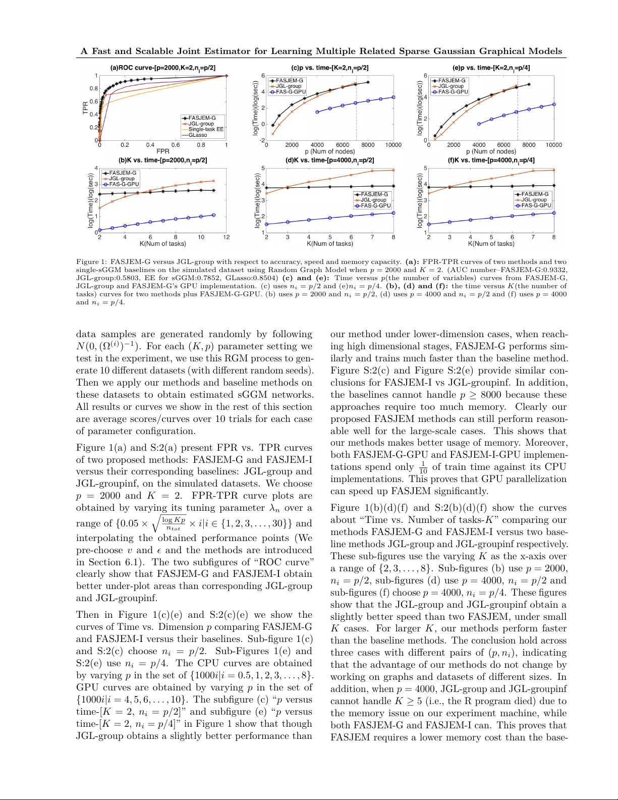
A F ast and Scalable Join t Estimator for Learning Multiple Related Sparse Gaussian Graphical Mo dels Beilun W ang Ji Gao Y anjun Qi Univ ersity of Virginia Univ ersity of Virginia Univ ersity of Virginia Abstract Estimating multiple sparse Gaussian Graphi- cal Mo dels (sGGMs) join tly for many related tasks (large K ) under a high-dimensional (large p ) situation is an imp ortan t task. Most previous studies for the join t estima- tion of m ultiple sGGMs rely on p enalized log-lik eliho o d estimators that inv olv e exp en- siv e and difficult non-smo oth optimizations. W e prop ose a nov el approac h, F ASJEM for fa st and s calable j oin t structure- e stimation of m ultiple sGGMs at a large scale. As the first study of joint sGGM using the Elemen- tary Estimator (EE) framew ork, our w ork has three ma jor contributions: (1) W e solv e F AS- JEM through an en try-wise manner which is parallelizable. (2) W e choose a proximal al- gorithm to optimize F ASJEM. This impro ves the computational efficiency from O ( K p 3 ) to O ( K p 2 ) and reduces the memory require- men t from O ( K p 2 ) to O ( K ) . (3) W e theo- retically prov e that F ASJEM achiev es a con- sisten t estimation with a con vergence rate of O ( log ( K p ) /n tot ) . On sev eral synthetic and four real-world datasets, F ASJEM sho ws sig- nifican t impro vemen ts ov er baselines on accu- racy , computational complexit y and memory costs. 1 In tro duction The past decade has seen a rev olution in collecting large- scale heterogeneous data from many scientific fields. F or instance, genomic technologies ha ve deliv ered fast and accurate molecular profiling data across many cel- lular contexts (e.g., cell lines or stages) from national pro jects like ENCODE[ 1 ]. Giv en such data, under- Pro ceedings of the 20 th In ternational Conference on Artifi- cial In telligence and Statistics (AIST A TS) 2017, F ort Laud- erdale, Florida, USA. JMLR: W&CP volume 54. Copyrigh t 2017 b y the author(s). standing and quan tifying v ariable graphs across m ulti- ple contexts is a fundamen tal analysis task. Such v ari- able graphs can significantly simplify net work-driv en studies ab out diseases or drugs[ 2 ]. The num b er of con texts those applications need to consider grows ex- tremely fast. F or example, the ENCODE [ 1 ] pro ject, b eing generated ov er ten y ears with con tributions from bio-labs across the world, con tains expression data from 147 differen t human cell t ypes (i.e., the n um b er of tasks K = 147 ) in 2016. Besides, the num b er of v ariables (de- noted as p ) is also quite large, ranging from thousands (e.g., gene) to h undreds of thousands (e.g., SNP[3]). W e form ulate this data analysis problem as join tly estimating K conditional dep endency graphs G (1) , G (2) , . . . , G ( K ) from data samples accumulated from K distinct conditions. F or homogeneous data samples from a given i -th condition, one typical ap- proac h in the literature is the sparse Gaussian Graphi- cal Mo del(sGGM)[ 4 , 5 , 6 ]. sGGM assumes data sam- ples are indep enden tly and iden tically drawn from N p ( µ ( i ) , Σ ( i ) ) , a multiv ariate normal distribution with mean µ ( i ) and cov ariance matrix Σ ( i ) . The graph struc- ture G ( i ) is enco ded by the sparsit y pattern of the in verse cov ariance matrix, also named precision matrix, Ω ( i ) . Ω ( i ) := ( Σ ( i ) ) − 1 . In G ( i ) an edge do es not connect j -th node and k -th node (i.e., conditional indep enden t) if and only if Ω ( i ) j k = 0 . sGGM imposes an ` 1 p enalt y on the parameter Ω ( i ) . F or heterogeneous data samples, rather than estimating sGGM of eac h condition sepa- rately , a m ulti-task form ulation that join tly estimates K differen t but related sGGMs can lead to a b etter generalization[7]. Most previous studies[ 8 , 9 , 10 , 11 , 12 , 13 , 14 , 15 ] for join t estimation of multiple sGGMs relied on optimiz- ing ` 1 regularized likelihoo d function plus an extra p enalt y function R 0 . This extra regularizer R 0 , which v aries in different estimators, enforces similarit y among m ultiple estimated netw orks. Since the p enalized like- liho od framework includes tw o regularization functions ( ` 1 + R 0 ), these approac hes cannot av oid the steps lik e SVD [ 8 ] and matrix multiplication [ 8 , 9 ]. Both steps need O ( K p 3 ) time complexity for computation. Be- A F ast and Scalable Join t Estimator for Learning Multiple Related Sparse Gaussian Graphical Models sides, most studies in this category require all tasks’ co- v ariance matrices to lo cate in the main memory[ 8 , 9 , 10 ] (for their optimization). Storing all elements needs O ( K p 2 ) memory space. As a result, this category of mo dels are difficult to scale up when the dimension p or the num b er of tasks K are large. In this pap er, w e prop ose a nov el mo del, namely fa st and s calable j oin t e stimator for m ultiple sGGM (F AS- JEM), for estimating multiple sGGMs jointly . Briefly sp eaking, this paper mak es the following con tributions: • No vel approac h: F ASJEM presen ts a new wa y of learning m ulti-task sGGMs by extending the elemen- tary estimator [16]. (Section 3) • F ast optimization: W e optimize F ASJEM through an en try-wise and group-entry-wise manner that can dramatically improv e the time complexity to O ( K p 2 ) . (Section 3 and Section 3.3) • Scalable optimization: The optimization of our estimators is scalable. W e reduce the memory cost to O ( K ) (i.e., requiring to store at most K en tries in the main memory). (Section 5) • Metho d v ariations: W e prop ose t wo v ariations of F ASJEM: (1) F ASJEM-G uses a group-2 norm to connect m ultiple sGGMs. (2) F ASJEM-I uses a group-infinite norm to connect multiple related sGGMs. Both metho ds show b etter p erformance o ver their corresponded “Join t graphical lasso” (JGL) baselines. (Section 3 and Section 6) • Con vergence rate: W e theoretically pro ve the con- v ergence rate of F ASJEM as O ( log ( K p ) /n tot ) . This rate shows the b enefit of joint estimation, which sig- nifican tly improv es the con vergence rate O ( log p n ) of single task sGGM (with n samples). (Section 5) • Ev aluation: F ASJEM is ev aluated using several syn thetic datasets and four real-world biomedical datasets. It p erforms better than the baselines not only on accuracy but also with resp ect to the time and storage requirements. (Section 6) A tt: Due to space limit, we hav e put details of certain con tents (e.g., pro ofs) in the app endix. Notations with “S:” as prefix in the num b ering mean the corresp onding con tents are in the app endix. F or example, full pro ofs are in Section S:8. Notations: W e fo cus on the problem of estimating K sGGMs from a p -dimensional aggregated dataset in the form of K differen t data matrices. X ( i ) n i × p describ es the data matrix for the i -th task, which includes n i data samples describ ed b y p differen t feature v ariables. The total n umber of data samples is n tot = K P i =1 n i . W e use notation Ω for the precision matrices and b Σ for the estimated cov ariance matrices. Giv en a p -dimensional v ector x = ( x 1 , x 2 , . . . , x p ) T ∈ R p , || x || 1 = P i | x i | repre- sen t the l 1 -norm of x . || x || ∞ = max i | x i | is the l ∞ -norm of x . || x || 2 = r P i x 2 i , ` 2 -norm of x . 2 Bac kground Single-task sGGM: The classic form ulation of sparse Gaussian Graphical model [ 6 ] for a single giv en task (or con text) (single sGGM) is the “graphical lasso” estima- tor (GLasso) [ 6 , 17 ] that solves the follo wing penalized maxim um lik eliho od estimation (MLE) problem: argmin Ω > 0 − log det (Ω)+ < Ω , Σ > + λ n || Ω || 1 (2.1) Elemen tary estimator for single sGGM (EE-sGGM): Recen tly the seminal study[ 18 ] gener- alized this formulation in to a so-called M-estimator framew ork: argmin θ L ( θ ) + λ n R ( θ ) (2.2) where R ( · ) represents a decomposable regularization function in [ 18 ] and L ( · ) represents a loss function (e.g., the negative log-lik eliho od function − L ( · ) in sGGM). Recen t studies[ 19 , 16 ] prop ose a new category of estima- tors named “Elementary estimator” 1 , whose solution ac hieves the same optimal conv ergence rate as Eq. (2.2) when satisfying certain conditions. These estimators ha ve the following general formulation: argmin θ R ( θ ) sub ject to: R ∗ ( θ − b θ n ) ≤ λ n (2.3) Where R ∗ ( · ) is the dual norm of R ( · ) , R ∗ ( v ) := sup u 6 =0 < u, v > R ( u ) = sup R ( u ) ≤ 1 < u, v > . (2.4) b θ n represen ts the bac kward mapping of θ . W e pro- vide detailed explanations of bac kward mapping and bac kward mapping for Gaussian case in the App endix Section S:1. F or sGGM, it is easy to deriv e Ω through the backw ard mapping on its cov ariance matrix Σ , whic h is Σ − 1 . Ho wev er, under the high-dimensional setting, when p > n , the sample cov ariance matrix b Σ is not full rank, therefore is not inv ertible. Thus the authors of [ 16 ] prop osed a proxy bac kward mapping on the cov ariance matrix b Σ under high-dimensional set- tings as ( T v ( b Σ )) − 1 . Here [ T v ( M )] ij := ρ v ( M ij ) where ρ v ( · ) is chosen to b e a soft-thresholding function. [ 16 ] pro ves that this appro ximation will not c hange the con vergence rate of sGGM estimation. Using Eq. (2.3), [ 16 ] proposed a new estimator for sGGM (the so-called elemen tary estimator for sGGM): argmin Ω || Ω || 1 sub ject to: || Ω − [ T v ( b Σ)] − 1 || ∞ ≤ λ n (2.5) This estimator has a closed-form solution[ 16 ] and has b een sho wn to b e more practical and scalable than GLasso in large-scale settings. v is a hyperparameter 1 W e denote this category of estimators as “elementary estimator” or “EE” in the rest of pap er. Beilun W ang, Ji Gao, Y anjun Qi whic h ensures that T v ( b Σ) is inv ertible. Multi-task sGGM (Multi-sGGM): F or join t esti- mation of multiple sGGMs, most studies fo cus on adding a second norm which enforces the group prop- ert y among multiple tasks. Previous studies on the join t estimation of multiple sGGMs can be summarized using Eq. (2.6), argmin Ω ( i )  0 K X i =1 ( − L (Ω ( i ) ) + λ n K X i =1 || Ω ( i ) || 1 + λ 0 n R 0 (Ω (1) , Ω (2) , . . . , Ω ( K ) ) (2.6) where Ω ( i ) denotes the precision matrix for i -th task. Ω ( i )  0 means that Ω ( i ) needs to b e a positive definite matrix. R 0 ( · ) represents the second p enalt y function for multi-tasking. Sup erposition structured estimator (SS estima- tor) : The ab o ve Eq. (2.6) is a sp ecial case (explained in Section 3) of the follo wing sup erp osition structured estimators [18]: argmin ( θ α ) α ∈ I L ( X α ∈ I θ α ) + X α ∈ I λ α R α ( θ α ) . (2.7) {R α ( · ) | α ∈ I } are a set of regularization functions and ( λ α ) α ∈ I are the regularization p enalties. The target parameter is θ = P α ∈ I θ α , a sup erp osition of θ α . Elemen tary superp osition-structured momen t estimator (ESS momen t estimator): Similar to Eq. (2.3), a recent study[ 20 ] extends the elemen tary estimator for sparse cov ariance matrices to the case of sup erposition-structured moments and named this extension as “Elem-Sup er-Moment” (ESM) estimator. 2 argmin θ 1 ,θ 2 ,...,θ | I | X α ∈ I λ α R α ( θ α ) Sub ject to: R ∗ α ( b θ − X α ∈ I θ α ) ≤ λ α ∀ α ∈ I . (2.8) 3 Metho d: A fast and scalable joint estimator for multi-sGGM The p enalized likelihoo d framew ork for multi-task sG- GMs in Eq. (2.6) inv olves a h ybrid of t wo regularization functions ( ` 1 + R 0 ). Studies in this direction cannot a void the expensive steps lik e SVD and matrix multipli- cation and also require to store K co v ariance matrices in the main memory . Since this pap er aims to de- sign a scalable joint estimator for multi-sGGM under large-scale settings, extending the elemen tary estima- tor of single-task sGGM [ 16 ] to m ulti-task form ulation b ecomes a natural choice. F or multi-task sGGMs, w e can denote that Ω tot = 2 [ 20 ] has prov ed that this class of ESM estimators ac hieves the same conv ergence rate as the corresp onding estimators (with the same superp osition of structures) using the penalized MLE formulation under certain conditions. (Ω (1) , Ω (2) , . . . , Ω ( K ) ) and Σ tot = (Σ (1) , Σ (2) , . . . , Σ ( K ) ) . Ω tot and Σ tot are b oth p × K p matrices (i.e., K p 2 param- eters to estimate). No w define an in verse function as in v ( A tot ) := ( A (1) − 1 , A (2) − 1 , . . . , A ( K ) − 1 ) , where A tot is a giv en p × K p matrix with the same structure as Σ tot . F urthermore, we add a new hyperparameter v ariable  = λ 0 n λ n . Let I = { 1 , 2 } and θ 1 = θ 2 = 1 2 Ω tot . W e can clearly tell that Eq. (2.6) is a sp ecial case of the superp osi- tion structured estimation in Eq. (2.7). The ESS (ele- men tary sup erp osition structured) momen t estimator (Eq. (2.8)) extends the elementary estimator of struc- tured cov ariance matrix to elementary sup erposition- structured estimator for estimating co v ariance matrices with a hybrid structure (e.g., sparse + low rank). This motiv ates us to prop ose the following elementary su- p erposition estimator for learning m ulti-task sGGM: argmin Ω tot || Ω tot || 1 +  R 0 (Ω tot ) s.t. || Ω tot − inv ( T v ( b Σ tot )) || ∞ ≤ λ n R 0∗ (Ω tot − inv ( T v ( b Σ tot ))) ≤ λ n (3.1) Here || · || ∗ 1 = || · || ∞ (the dual norm of l 1 -norm is l ∞ - norm). R 0 ( · ) represents a regularizer on Ω tot to enforce that { Ω ( i ) } share certain similarity . R 0 ∗ ( · ) is the dual norm of R 0 ( · ) . W e name this nov el formulation as F ASJEM. By v arying R 0 ( · ) , we can get a v ariety of F ASJEM estimators. Section 5 theoretically pro ves the con vergence rate of F ASJEM as O ( log ( K p ) /n tot ) . Our theory pro of is inspired by the ESS moment estimator [ 20 ], the SS estimator [21] and the EE-sGGM [16]. 3.1 Metho d I: F ASJEM-G F or multi-task regularization, the first R 0 ( · ) we try is the G , 2 -norm (i.e., R 0 ( · ) = || · || G , 2 ). This norm is in- spired by JGL-group lasso[ 8 ]. G , 2 -norm constrains the parameters in the same group to hav e the same lev el of sparsit y . In multi-task sGGMs, group set G := { g j,k } , where g j,k = { Ω ( i ) j,k | i = 1 , . . . , K } . Supp ose g is an arbi- trary group in group set G and totally we hav e p 2 groups. || Ω tot || G , 2 = p P j =1 p P k =1 || (Ω (1) j,k , Ω (2) j,k , . . . , Ω ( i ) j,k , . . . , Ω ( K ) j,k ) || 2 . When R 0 ( · ) = ||· || G , 2 , we name Eq. (3.1) as F ASJEM-G (short form of F ASJEM-Group2). W e solv e F ASJEM-G using a parallel proximal based optimization formula- tion from[ 22 ]. Algorithm 1 summarizes the detailed optimization steps and the four proximit y op erators implemen ted on GPU are listed in T able 1 3 . The opti- mization sequence of Algorithm 1 conv erges Q-linearly (See Eq. (S:2–10)). 3 The non-GPU version of the four proximit y operators are in Eq. (S:2–2) to Eq. (S:2–5). A F ast and Scalable Join t Estimator for Learning Multiple Related Sparse Gaussian Graphical Models 3.2 Metho d I I: F ASJEM-I As sho wn in Section 4, most previous models for m ulti- task sGGMs v aried the second norm R 0 to obtain dif- feren t mo dels. Similarly w e can easily change R 0 ( · ) in Eq. 3.1 in to any other desired norm to extend our F ASJEM. F or instance, w e can c hange R 0 ( · ) to group- infinit y norm || · || G , ∞ . || Ω tot || G , ∞ = p P j =1 p P k =1 || (Ω (1) j,k , Ω (2) j,k , . . . , Ω ( i ) j,k , . . . , Ω ( K ) j,k ) || ∞ . This norm is inspired b y a multi-task sGGM prop osed b y [ 11 ]. When using group-infinity norm, we get F ASJEM-I(short for F ASJEM-Groupinf). W e can deriv e the optimization for F ASJAM-I by changing t wo pro ximities in Algorithm 1. Considering that the original formulation in [ 11 ] is similar with JGL[ 8 ], in the rest of this paper, w e call the mo del from [ 11 ] as JGL-groupinf or JGL-I (the corresp onded baseline for F ASJEM-I). 3.3 Pro ximal Algorithm for Optimization Eq. (3.1) includes a con vex programming task since the norms we c ho ose are con vex. By simplifying notations and adding another parameter, we reform ulate it to: argmin θ 1 ,θ 2 f 1 ( θ 1 ) + f 2 ( θ 2 ) sub ject to : || θ 1 − inv ( T v ( b Σ tot )) || ∞ ≤ λ n R 0∗ ( θ 2 − inv ( T v ( b Σ tot ))) ≤ λ n θ 1 = θ 2 (3.2) Where f 1 ( · ) = || · || 1 and f 2 ( · ) =  || · || G , 2 . Then w e con vert Eq. (3.2) to the following equiv alent and distributed formulation: argmin θ 1 ,θ 2 ,θ 3 ,θ 4 f 1 ( θ 1 ) + f 2 ( θ 2 ) + f 3 ( θ 3 ) + f 4 ( θ 4 ) sub ject to: θ 1 = θ 2 = θ 3 = θ 4 (3.3) Here f 3 ( θ ) = I {|| θ − inv ( T v (Σ tot )) || ∞ ≤ λ n } ( θ ) and f 4 ( θ ) = I {|| θ − inv ( T v (Σ tot )) || ∗ G , 2 ≤ λ n } ( θ ) . I C ( · ) represents the in- dicator function of a conv ex set C as I C ( x ) = 0 when x ∈ C . Otherwise I C ( x ) = ∞ . T o solv e Eq. (3.3), w e c ho ose a parallel proximal based algorithm[ 22 ] summa- rized in Algorithm 1. Besides the distributed nature, the proximal algorithm also bring in the b enefit that man y pro ximity op erators are entry-wise op erators for the targeted parameters. The four pro ximal op erators for four functions { f 1 , f 2 , f 3 , f 4 } (for CPU platform im- plemen tation) are included in the Equations Eq. (S:2– 2) to Eq. (S:2–5) in Section S:2. With the benefits as pro ximal op erators, Eq. (S:2–2) and Eq. (S:2–4) are en try-wise and Eq. (S:2–3) and Eq. (S:2–5) are group en try-wise. 3.4 GPU Implemen tation of F ASJEM-G W e further revise Algorithm 1 to take adv an tage of the adv anced computational architecture–GPU. This algo- rithm cannot b e directly parallelized on GPU, because GPU is slo w for multiple branc hes based predictions. T able 1: F our proximit y operators implemented on GPU platform. [ prox γ f 1 ( x )] ( i ) j,k max(( x ( i ) j,k − γ ) , 0)+ min(0 , ( x ( i ) j,k + γ )) prox γ f 2 ( x g ) x g max((1 − γ || x g || 2 ) , 0) [ prox γ f 3 ( x )] ( i ) j,k min(max( x ( i ) j,k − a ( i ) j,k , − λ n ) , λ n ) + a ( i ) j,k prox γ f 4 ( x g ) max( λ n || x g − a g || 2 , 1)( x g − a g ) + a g Therefore, we con vert those four op erators pro x ( · ) in Algorithm 1 in to single soft-threshold based operators whic h only include simple algorithmic op erations like + or max . These op erators can b e easily parallelized on GPU[ 23 ]. The four proxi mity operators w e use to implemen t F ASJEM-G on GPU are summarized in T able 1. More details are included in Section S:2. Algorithm 1 P arallel pro ximal algorithm 4 input K giv en data blocks X (1) , X (2) , . . . , X ( K ) . Hyper- parameter: α ,  , v , λ n and γ . Learning rate: 0 < ρ < 2 . Max iteration num b er iter . output Ω tot 1: Compute Σ tot from X (1) , X (2) , . . . , X ( K ) 2: Initialize θ 0 = in v ( T v (Σ tot )) , θ 0 j = in v ( T v (Σ tot )) for j ∈ { 1 , 2 , 3 , 4 } and a = in v ( T v (Σ tot )) . 3: for i = 0 to iter do 4: p i 1 = pro x 4 γ f 1 θ i 1 5: p i 2 = pro x 4 γ f 2 θ i 2 6: p i 3 = pro x 4 γ f 3 θ i 3 7: p i 4 = pro x 4 γ f 4 θ i 4 8: p i = 1 4 ( 4 P j =1 θ i j ) 9: for j = 1 , 2 , 3 , 4 do 10: θ i +1 j = θ i j + ρ (2 p i − θ i − p i j ) 11: end for 12: θ i +1 = θ i + ρ ( p i − θ i ) 13: end for 14: Ω tot = θ iter output Ω tot 4 Connecting to Relev an t Studies Estimators for Single task sGGM: Sparse GGM is a highly active topic in the recen t literature. Roughly sp eaking, there exist three major categories of estima- tors for sGGM. A k ey class of estimators is based on the regularized maximum likelihoo d optimization. The p op- ular estimator “graphical lasso”(GLasso) considers max- imizing a ` 1 p enalized normal likelihoo d [ 6 , 17 , 24 , 25 ]. As the second t yp e, CLIME estimator[ 26 ] learns sGGM b y solving a constrained ` 1 optimization. The CLIME form ulation can be conv erted into m ultiple subproblems of linear programming and has sho wn more fa vorable theoretical prop erties than GLasso. The linear pro- gramming while conv ex, is computationally exp ensiv e for large-scale tasks. Recently as a third group of stud- 4 F our proximit y op erators used on GPU are defined in T able 1. Hyp erparameters are explained in Section 6. Here j, k = 1 , . . . , p , i = 1 , . . . , K and g ∈ G . Beilun W ang, Ji Gao, Y anjun Qi ies, soft-thresholding based elementary estimators[ 16 ] ha ve been introduced for inferring undirected sparse Graphical mo dels. This paper mostly follows the third category . Besides, there exists quite a n umber of recen t studies trying to scale up single sGGM to a large scale. F or example, the BigQUIC algorithm [ 27 ] prop oses an asymptoticly quadratic optimization to estimate sGGM. The elementary estimator [ 16 ] of sGGM is an adv anced v ersion of BigQUIC. Multi-sGGM: Previous Lik eliho o d based Esti- mators. Most previous metho ds to jointly estimate m ultiple sGGMs can be form ulated using the p enalized MLE Eq. (2.6), including for instance, (1) Joint graph- ical lasso (JGL-group uses G , 2 -norm in Section 3.1 [ 8 ]), (2) No de-perturb ed JGL [ 9 ], (3) Simone [ 10 ], and (4) m ulti-task sGGM prop osed b y [ 11 ]. These metho ds differ with respect to the second regularization function R 0 ( · ) they used to enforce their assumption of similarit y among tasks. Optimization and Computational Comparison: W e use JGL-group and the mo del prop osed by [ 11 ] (w e name it as JGL-groupInf ) as baselines in our exper- imen ts. As w e mentioned in Section 1, the b ottlenec k of optimizing multi-sGGM in JGL-group is the step of SVD that needs O ( K p 3 ) time complexity and re- quires storing K co v ariance matrix ( O ( K p 2 ) memory cost). Differen tly , JGL-Groupinf chose a co ordinate descen t metho d and prov ed that their optimization is equiv alent to p sequences of quadratic subproblems, eac h of whic h costs O ( K 3 p 3 ) computation. Therefore the total computational complexity of JGL-Groupinf is O ( K 3 p 4 ) . Besides, this co ordinate descen t metho d needs to store all K co v ariance matrices in the main memory( O ( K p 2 ) memory cost). T able 2 compares our mo del with tw o baselines in terms of time and space cost. Solving our mo del relies totally on en try-wise and group-entry-wise procedures. Its time complexity is O ( K p 2 ) . This is muc h faster than the baselines, esp ecially in high-dimensional settings (T able 2). 5 Moreo ver, in our optimization, learning the parameters for each group { Ω ( i ) j,k | i = 1 , . . . , K } do es not rely on other groups. This means we only need to store K en tries of the same group in the memory for computing Eq. (S:2–4) and Eq. (S:2–5). The space complexity O ( K ) is muc h smaller than previous metho ds’ O ( K p 2 ) requiremen t. 6 The comparisons are in T able 2. 5 Note that the discussion of time complexit y is for each iteration in optimization. W e show the Q-linear conv ergence for all first-order multi-task sGGM estimators in Eq. (S:2– 10). Since the baselines and our metho ds all use first-order optimization, we assume the num b er of iterations is the same among all methods. 6 W e hav e pro vided a GPU implementation of F ASJEM in Section 3.3. Although SVD or matrix in version can also b e sp eed up by GPU parallelization, these metho d T able 2: Comparison to Previous multi-sGGM metho ds References Computational Com- plexity Memory Cost JGL-Group [8] O ( K p 3 ) O ( K p 2 ) JGL-GroupInf [11] O ( K 3 p 4 ) O ( K p 2 ) F ASJEM Mo d- els O ( K p 2 ) (if paralleling completely , O ( K ) ) O ( K ) Previous Studies using Elemen tary based Esti- mators: Most previous studies of multi-sGGMs follo w the p enalized MLE framework. F ew w orks of Multi- task sGGM follow the CLIME formulation, since it is not easy to transfer tw o regularizers in to the CLIME form ulation (summarized in T able S:1). Based on the authors’ knowledge, no previous multi-sGGM studies ha ve follo wed the elementary estimators(EE) form ula- tion. As a simple soft-thresholding based estimator, elemen tary estimators (EE) ha ve been used for other tasks as well. T able S:1 summarizes three different t yp es of previous tasks for which EE can b e applied: high-dimensional regression, single sGGM and m ulti- sGGM. F or comparison, we sho w ho w these tasks hav e b een solved through the p enalized lik eliho o d framework in the second column and use the the third column to sho w studies following the CLIME formulation. Con vergence Rate Analysis: Although previous join t sGGMs work well on datasets whose K and p are relatively small, tw o important questions re- main unanswered: (1) what’s the statistical conv er- gence rate of these joint estimators? and (2) what’s the b enefits of joint learning? The conv ergence rate of estimating single-task sGGM has b een well in vestigated[ 6 , 17 , 24 , 25 ]. These studies prov ed that the estimator of single-task sGGM holds a consistent con vergence rate O ( q log p n ) if given n data samples. Ho wev er, none of the previous joint-sGGM studies pro vide suc h theoretical analysis. Experimental ev al- uations in previous joint-sGGM pap ers hav e shown b etter p erformance of running joint estimators ov er running single-task sGGM estimators on each dataset separately . How ever, it hasn’t b een prov en that theo- retically this joint estimation is better. W e successfully answ er these tw o remaining questions in Section 5. 5 Theoretical Analysis In this section, we prov e that our estimator can b e optimized asynchronously in a group entry-wise man- ner. W e also provide the pro of of the theoretical error b ounds of F ASJEM. cannot av oid the O ( K p 2 ) memory cost, whic h is a huge b ottlenec k for large-scale problems. In Section 5 we prov e that our estimator is completely group en try-wise and asyn- c hronously optimizable, this makes F ASJEM only require O ( K ) memory storage. A F ast and Scalable Join t Estimator for Learning Multiple Related Sparse Gaussian Graphical Models 5.1 Group en try-wise and parallelizing optimizable Theorem 5.1. ( F ASJEM is Gr oup entry-wise optimizable ) Supp ose we use F ASJEM to infer mul- tiple inverse of c ovarianc e matric es summarize d as b Ω tot . { b Ω ( i ) j,k | i = 1 , . . . , K } describ es a gr oup of K en- tries at ( j, k ) p osition. V arying j ∈ { 1 , 2 , . . . , p } and k ∈ { 1 , 2 , . . . , p } , we have total ly p × p gr oups. If these gr oups ar e indep endently estimate d by F ASJEM, then we have, p [ j =1 p [ k =1 { b Ω ( i ) j,k | i = 1 , . . . , K } = b Ω tot . (5.1) Pr o of. Eq. (S:2–6) and Eq. (S:2–8) are soft- thresholding based operators on each en try . Eq. (S:2–7) and Eq. (S:2–9) are soft-thresholding op erators on each group of entries. Corollary 5.2. W e c an de c omp ose F ASJEM into p × p subpr oblems that ar e indep endent fr om e ach other, and solve e ach subpr oblem at a time. Ther efor e our estima- tor only r e quir es O ( K ) memory stor age for c omputa- tion. This corollary prov es the claims w e show ed in section 4. Through Theorem (5.1), it is imp ortan t to notice that the optimization on multiple groups of entries can b e totally parallelized . 5.2 Theoretical error b ounds In this subsection, w e first pro vide the error bounds for elemen tary sup er-position estimator (ESS estimator) under I = { 1 , 2 } . W e then use this general b ound to pro ve the error b ound for F ASJEM-G. All the pro ofs are included in Section S:8. W e also include the error b ounds for elementary estimator (EE) in Section S:7. Extension to ESS: F or the m ultiple-task case, we need to consider t wo or more regularization functions. F or instance, in F ASJEM-G we assume the sparsity of parameter and the group sparsity among tasks. Since w e only consider the mo dels with tw o regularization function, we consider the error bounds of the following elemen tary sup er-p osition estimator formulation in the rest of the section. argmin θ 1 ,θ 2 λ 1 R 1 ( θ 1 ) + λ 2 R 2 ( θ 2 ) sub ject to: R ∗ i ( b θ n − ( θ 1 + θ 2 )) ≤ λ i , i = 1 , 2 (5.2) This equation restricts the num b er of penalty functions to 2 . Similar to the single-task error b ounds (in Sec- tion S:7) , w e naturally extend condition (C2) to the follo wing condition: (C3) pro j M ⊥ i ( θ ∗ i ) = 0 , i = 1 , 2 . W e b orrow the follo wing condition from [ 21 ], which is a structural incoherence condition ensuring that the non-in terference of different structures. (C4) Let Φ := max { 2 + 3 λ 1 Ψ 1 ( ¯ M 1 ) λ 2 Ψ 2 ( ¯ M 2 ) , 2 + 3 λ 2 Ψ 2 ( ¯ M 2 ) λ 1 Ψ 1 ( ¯ M 1 ) } . max { σ max ( P ¯ M 1 P ¯ M 2 ) , σ max ( P ¯ M 1 P ¯ M ⊥ 2 ) σ max ( P ¯ M ⊥ 1 P ¯ M ⊥ 2 ) } ≤ 1 16Φ 2 where P ¯ M is the matrix corresp onding to the pro jection op erator for the subspace ¯ M . The definition of Ψ( · ) are included in Definition (S:7.1). With these t wo conditions, we hav e the follo wing theo- rem: Theorem 5.3. Supp ose that the true p ar ameter θ ∗ satisfies the c onditions (C3)(C4) and λ i ≥ R ∗ i ( b θ − θ ∗ ) , then the optimal p oint b θ of Eq. (5.2) has the fol lowing err or b ounds: R ∗ i ( b θ − θ ∗ ) ≤ 2 λ i , i = 1 , 2 (5.3) R i ( b θ − θ ∗ ) ≤ 32 λ i (max i λ i Ψ( ¯ M i )) 2 , i = 1 , 2 (5.4) || b θ − θ ∗ || F ≤ 8 max i λ i Ψ( ¯ M i ) (5.5) Notice that for F ASJEM-G mo del, R 1 = || · || 1 and R 2 = || · || G , 2 . Based on the results in[ 18 ], Ψ( ¯ M 1 ) = √ s and Ψ( ¯ M 2 ) = √ s G , where s is the n umber of nonzero en tries in Ω tot and s g is the n um b er of groups in which there exists at least one nonzero entry . Clearly s > s g . Also in practice, to utilize group information, we hav e to c ho ose hyperparameter λ n > λ 0 n ( λ 1 > λ 2 in Eq. (5.5)). Therefore by Theorem (5.3), w e hav e the following theorem, Theorem 5.4. Supp ose that R 1 = || · || 1 and R 2 = || · || G , 2 and the true p ar ameter Ω ∗ tot satisfies the c onditions (C3)(C4) and λ i ≥ R ∗ i ( b Ω tot − Ω ∗ tot ) , then the optimal p oint b Ω tot of Eq. (3.1) has the fol lowing err or b ounds: || b Ω tot − Ω ∗ tot || F ≤ 8 √ sλ n . W e then deriv e a corollary of Theorem (5.4) for F ASJEM-G. A prerequisite is to show that inv ( T v ( b Σ tot )) is w ell-defined. The follo wing conditions define a broad class of sGGM that satisfy the require- men t. Similar results are also in tro duced by[16]. Conditions for elementary estimator of sGGM: C-MinInf Σ The true parameter Ω ∗ tot of Eq. (5.2) has b ounded induced op erator norm, i.e., ||| Ω ( i ) ∗ ||| ∞ := sup w 6 =0 ∈ R p || Σ ( i ) ∗ w || ∞ | w | ∞ ≤ κ 1 ∀ i . C-Sparse Σ The true m ultiple co v ariance matrices Σ ∗ tot := inv (Ω ∗ tot ) are “appro ximately sparse” along the lines [ 28 ] : for some p ositiv e constan t D , Σ ( i ) j,j ∗ ≤ D for all diagonal en tries. Moreov er, for some 0 ≤ q < 1 and c 0 ( p ) , max i p P j =1 | Σ ( i ) j,k ∗ | q ≤ c 0 ( p ) ∀ i . If q = 0 , then this condition reduce to Σ ∗ b eing sparse. W e additionally require inf w 6 =0 ∈ R p | Ω ( i ) ∗ w | ∞ | w | ∞ ≥ κ 2 . Beilun W ang, Ji Gao, Y anjun Qi Error b ounds of F ASJEM-group: In F ASJEM, θ ∗ 1 = θ ∗ 2 = 1 2 θ ∗ . θ i is the parameter w.r.t a subspace pair ( M i , ¯ M ⊥ i ) , where i = 1 , 2 . Here R 1 = || · || 1 and R 2 = || · || G , 2 . W e assume the true parameter θ ∗ satisfies C-MinInf Σ and C- Sparse Σ conditions. Using the ab ov e theorems, we ha ve the following corollary: Corollary 5.5. If we cho ose hyp erp ar ameters λ 0 n < λ n . L et v := a q log p 0 n tot for p 0 = max ( K p, n tot ) . Then for λ n := 4 κ 1 a κ 2 q log p 0 n tot and n tot > c log p 0 , with a pr ob ability of at le ast 1 − 2 C 1 exp ( − C 2 K p log ( K p )) , the estimate d optimal solution b Ω tot has the fol lowing err or b ound: || b Ω tot − Ω ∗ tot || F ≤ 32 4 κ 1 a κ 2 q s log p 0 n tot } wher e a , c , κ 1 and κ 2 ar e c onstants. The conv ergence rate of single-task sGGM is O ( log p/n i ) . In high-dimensional setting, p 0 = K p since K p > n tot . Assuming n i = n tot K , the con vergence rate of single sGGM is O ( K log p/n tot ) . Clearly , since K log p > log ( K p ) , the con vergence rate of F ASJEM is b etter than single-task sGGM. 6 Exp erimen t Multiple simulated datasets and four real-world biomed- ical datasets are used to ev aluate F ASJEM. 6.1 Exp erimen tal Settings Baseline: W e compare (1)F ASJEM-G versus JGL- group [ 8 ]; (2)F ASJEM-I v ersus JGL-groupinf [ 11 ]. This is b ecause the specific F ASJEM estimator and its base- line share the same second-penalty function. 7 Three ev aluation metrics are used for suc h comparisons. • Precision: W e use the edge-level false p ositiv e rate (FPR) and true p ositiv e rate (TPR) to measure the pre- dicted graphs versus true graph. Rep eating the pro cess 10 times, we obtain av erage metrics for each metho d we tests. Here, FPR = FP FP + TN and TPR = TP TP + FN . TP (true positive) and TN (true negativ e) mean the num b er of true nonzero entries and the num b er of true zero en- tries estimated by the predicted precision matrices. The FPR vs. TPR curv e sho ws multi-point p erformance of a metho d ov er a range of the tuning parameter. The bigger the area under a FPR-TPR curve, the better a metho d has ac hieved ov erall. • Sp eed: The time ( log (second)) betw een the whole program’s start and end indicates the sp eed of a cer- tain metho d under a specific configuration of hyper- parameters. T o b e fair, w e set up tw o types of com- parisons. The first one fixes the num b er of tasks ( K ) but v aries the dimension ( p ) . This shows the p erformance of eac h method under a high-dimensional setting. The other t yp e fixes the dimension ( p ) but v aries the num b er of tasks ( K ) . This measures the p erformance of each 7 Since single-sGGM EE has a closed-form solution (i.e., no iterativ e steps are needed in optimization), w e do not include it as baseline. metho d when ha ving a large num b er of tasks. • Memory: F or each metho d, we v ary the num b er of tasks ( K ) and the dimension ( p ) un til a specific metho d termi- nates due to the “out of memory” error. This measures the memory capacity of the corresp onding method. Our implementation: W e implement F ASJEM on t wo differen t arc hitectures: (1)CPU only and (2)GPU 8 . Similar to the JGL-group from [ 8 ], we implemen t the CPU version F ASJEM-G and F ASJEM-I with R. W e c ho ose torch7 [ 29 ] (LUA based) to program F ASJEM on GPU machine. 9 Selection of hyper-parameters: In this experiment, w e need to c ho ose the v alue of three hyper-parameters. The first one v is unique for elementary-estimator based sGGM mo dels. The second λ n (in some mo dels also noted as λ 1 ) is the main h yp er-parameter w e need to tune. The third  equals to λ 0 n λ n (The notation λ 2 is normally used in related works instead of λ 0 n ). • v : W e pre-choose v in the set { 0 . 001 i | i = 1 , 2 , . . . , 1000 } to guaran tee T v (Σ tot ) is inv ertible. • λ n 10 : Recent research studies from [ 18 ] and [ 16 ] conclude that the regularization parameter λ n i of a single task with n i samples should b e chosen with λ n i ∝ q log p n i . Com bining this result and our con vergence rate analysis in Section 5, we choose λ n = α q log K p n tot where α is a h yp er-parameter. The h yp erparameter γ in Algorithm 1 equals to λ n . •  : W e select the b est  from the set { 0 . 1 i | i = 1 , 2 , . . . , 10 } using cross-v alidation. 6.2 Exp erimen ts on simul ated datasets Using the following “Random Graph Model”(RGM), w e first generate a set of synthetic multiv ariate Gaussian datasets, each of whic h includes samples of K tasks describ ed by p v ariables. F rom [ 25 ], this “Random Graph Mo del" assumes Ω ( i ) = B ( i ) + δ ( i ) I , where eac h off-diagonal entry in B ( i ) is generated indep endently , equals to 0.5 with probability 0 . 05 i and, equals to 0 with probabilit y 1 − 0 . 05 i . δ ( i ) is selected large enough to guaran tee the p ositiv e definiteness of precision matrix. F or each case of p , we use this mo del to generate K random sparse graphs. F or eac h graph (task), n = p/ 2 8 Information of Exp erimen t Machines: The machine that w e use for exp erimen ts includes Intel(R) Core(TM) i7-3770 CPU @ 3.40GHz with a 8GB memory . The GPU that we use for exp erimen ts is Nvidia T esla K40c with 2880 cores and 12GB memory . 9 Though the ideal memory requirement of F ASJEM is only O ( K ) , IO costs should also b e taken into account in real implementations. As b eing prov ed, Ω tot is group-entry- wise optimizable. The parameter groups are indep enden tly estimated in the parallelized style. When implementing F ASJEM in a single machine (our experimental setting), w e prefer to c ho ose smaller m to mak e full use of the main memory , where m is the n umber of parameter groups which are estimated at the same time. 10 λ n = 0 . 1 used for time and memory experiments A F ast and Scalable Join t Estimator for Learning Multiple Related Sparse Gaussian Graphical Mo dels Figure 1: F ASJEM-G v ersus JGL-group with resp ect to ac curacy , sp eed and memory ca p ac it y . (a): FPR-TPR curv es of t w o metho ds and t w o single-sGGM baselines on the sim ulated dataset using Random Graph M o del when p = 2000 and K = 2 . (A UC n um b er–F ASJEM-G:0.9332 , JGL-group:0.5803, EE for sGGM:0.7852 , GLasso:0.8504) (c) and (e): Time v ersus p (the n um b e r of v ariables) curv es from F ASJEM-G, JGL-group and F ASJEM-G’s GPU implemen tation. (c) uses n i = p/ 2 and (e) n i = p/ 4 . (b), (d) and (f ): the time v ersus K (the n um b er of tasks) curv es for t w o metho ds plus F ASJEM-G- GPU. (b) uses p = 2000 and n i = p/ 2 , (d) uses p = 4000 and n i = p/ 2 and (f ) uses p = 4000 and n i = p/ 4 . data samples are generated randomly b y follo wing N (0 , (Ω ( i ) ) − 1 ) . F or eac h ( K , p ) parameter setting w e test in the exp erimen t, w e use this R GM pro ces s to gen- erate 10 differen t datasets (with differen t random seeds). Then w e apply our metho ds and bas eline metho ds on these datasets to obtain estimated sGGM net w orks. All results or curv es w e sho w in the rest of this s ection are a v erage scores/curv es o v er 10 trials for eac h case of parameter configuration. Figure 1(a) and S :2(a) prese n t FPR vs. TPR curv es of t w o p rop osed metho ds: F ASJEM-G an d F ASJEM-I v ersus their corresp onding baselin es: JGL-group and JGL-groupinf, on the sim ulated datas ets. W e c ho ose p = 2000 and K = 2 . FPR-TPR curv e pl ots are obtained b y v arying its tuning par ameter λ n o v er a range of { 0 . 05 × q log K p n tot × i | i ∈ { 1 , 2 , 3 , . . . , 30 }} and in terp olating the obtained p erformance p oin ts (W e pre-c ho ose v and  and the me tho ds are in tro duced in Section 6.1). The t w o sub figures of “R OC curv e” clearly sho w that F ASJEM-G and F ASJEM-I obtain b etter under-plot areas th an corres p onding JGL-group and JGL-groupinf. Then in Figure 1(c )(e) and S:2(c)(e) w e sho w the curv e s of Time vs. Dimension p comparing F ASJEM-G and F ASJEM-I v ersus their baselines. Sub-figure 1(c) and S: 2(c) c ho ose n i = p/ 2 . Sub-Figures 1(e) and S:2(e) use n i = p/ 4 . The CPU curv es are obtained b y v arying p in the set of { 1000 i | i = 0 . 5 , 1 , 2 , 3 , . . . , 8 } . GPU curv es are obtained b y v arying p in the set of { 1000 i | i = 4 , 5 , 6 , . . . , 10 } . The subfigure (c) “ p v ersus time-[ K = 2 , n i = p/ 2 ]” and subfigure (e) “ p v ersus time-[ K = 2 , n i = p/ 4 ]” in Figure 1 sho w that th ough JGL-group obtains a sligh tly b etter p erforman ce than our metho d un der lo w er-dimension c ases, wh en reac h - ing high dimensional stages, F ASJEM-G p erforms sim- ilarly an d trains m uc h faster than the baselin e metho d. Figure S:2(c) and Figure S:2(e) pro vide similar con- clusions for F ASJEM-I vs JGL-groupinf. In addition, the bas elines cannot handle p ≥ 8000 b ecause thes e approac hes require to o m uc h memory . Clearly our prop osed F ASJEM metho d s can still p erform reason- able w ell for the lar ge-scale cas es. Th is sho ws that our metho ds mak es b etter usage of memory . Moreo v er, b oth F ASJEM-G-GPU and F ASJEM-I-GPU implemen- tations s p end only 1 10 of train time against its CPU implemen tations. This pro v es that GPU parallelization can sp eed up F ASJEM significan tly . Figure 1(b)(d)(f ) and S:2(b)(d)(f ) sh o w the curv es ab out “Time vs. Num b er of tasks- K ” comparing our metho d s F ASJEM-G and F ASJEM-I v ersus t w o base- line metho ds JGL-group and JGL-groupinf resp ectiv ely . These sub-figures use the v arying K as the x-axis o v er a range of { 2 , 3 , . . . , 8 } . Sub-figures (b) use p = 2000 , n i = p/ 2 , s ub-figures (d) use p = 4000 , n i = p/ 2 and sub-figures (f ) c h o ose p = 4000 , n i = p/ 4 . These figures sho w that the JGL-group and JGL-grou pinf obtain a sligh tly b etter sp ee d than t w o F ASJEM, under small K cases. F or larger K , our metho ds p erf orm faster than the baseline metho ds. The conclus ion hold across three cases with differ en t pairs of ( p, n i ) , indicatin g that the adv an tage of our metho ds do not c hange b y w orking on graphs and datasets of differen t sizes. In addition, when p = 4000 , JGL-group and JGL-groupinf cannot han dle K ≥ 5 (i.e., the R program di ed) due to the memory issue on our exp erimen t mac hi ne, while b oth F ASJEM-G and F ASJEM-I can. This pro v es that F ASJE M requires a lo w er memory cost than the base- Beilun W ang, Ji Gao, Y anjun Qi lines. In all subfigures (b), (d) and (f ), F ASJEM curves are roughly linear. The exp erimen tal results match with the computational complexity analysis we ha ve p erformed in T able 2 (the computation cost of F AS- JEM is linear to K). Moreov er, subfigures (b), (d) and (f ) sho w that b oth F ASJEM-G-GPU and F ASJEM-I- GPU implemen tations spend only 1 10 time of their CPU implemen tations respectively . This confirms that GPU- parallelization can sp eed up F ASJEM significantly . F urthermore in Section S:6, w e compare F ASJEM-G and JGL-group on four different real-world datasets. F ASJEM-G consistently outperforms JGL-group on all four datasets in reco vering more known edges. References [1] ENCODE Pro ject Consortium et al. An integrated encyclop edia of dna elements in the h uman genome. Natur e , 489(7414):57–74, 2012. [2] T rey Ideker and Nev an J Krogan. Differential net- w ork biology . Mole cular systems biolo gy , 8(1):565, 2012. [3] Tim Beck, Robert K Hastings, Sirisha Gollapudi, Rob ert C F ree, and Anthon y J Bro ok es. Gwas cen tral: a comprehensive resource for the compar- ison and interrogation of genome-wide asso ciation studies. Eur op e an Journal of Human Genetics , 22(7):949–952, 2014. [4] Steffen L Lauritzen. Gr aphic al mo dels . Oxford Univ ersity Press, 1996. [5] Kan tilal V arichand Mardia, John T Ken t, and John M Bibby . Multiv ariate analysis. 1980. [6] Ming Y uan and Yi Lin. Mo del selection and estima- tion in the gaussian graphical mo del. Biometrika , 94(1):19–35, 2007. [7] Ric h Caruana. Multitask learning. Machine le arn- ing , 28(1):41–75, 1997. [8] P atrick Danaher, Pei W ang, and Daniela M Wit- ten. The joint graphical lasso for inv erse co v ari- ance estimation across multiple classes. Journal of the R oyal Statistic al So ciety: Series B (Statistic al Metho dolo gy) , 2013. [9] Karthik Mohan, Palma London, Maryam F azel, Su-In Lee, and Daniela Witten. No de-based learn- ing of multiple gaussian graphical mo dels. arXiv pr eprint arXiv:1303.5145 , 2013. [10] Julien Chiquet, Y ves Grandv alet, and Christophe Am broise. Inferring multiple graphical structures. Statistics and Computing , 21(4):537–553, 2011. [11] Jean Honorio and Dimitris Samaras. Multi-task learning of gaussian graphical mo dels. In Pr o c e e d- ings of the 27th International Confer enc e on Ma- chine L e arning (ICML-10) , pages 447–454, 2010. [12] Jian Guo, Eliza veta Levina, George Michailidis, and Ji Zh u. Joint estimation of multiple graphical mo dels. Biometrika , page asq060, 2011. [13] Bai Zhang and Y ue W ang. Learning structural c hanges of gaussian graphical models in con trolled exp erimen ts. arXiv pr eprint arXiv:1203.3532 , 2012. [14] Yi Zhang and Jeff G Schneider. Learning multiple tasks with a sparse matrix-normal p enalt y . In A d- vanc es in Neur al Information Pr o c essing Systems , pages 2550–2558, 2010. [15] Y unzhang Zhu, Xiaotong Shen, and W ei P an. Structural pursuit ov er multiple undirected graphs. Journal of the A meric an Statistic al A sso ciation , 109(508):1683–1696, 2014. [16] Eunho Y ang, Aurélie C Lozano, and Pradeep K Ra vikumar. Elementary estimators for graphi- cal mo dels. In A dvanc es in Neur al Information Pr o c essing Systems , pages 2159–2167, 2014. [17] On ureena Banerjee, Laurent El Ghaoui, and Alexandre d’Aspremont. Mo del selection through sparse maximum lik eliho od estimation for m ulti- v ariate gaussian or binary data. The Journal of Machine L e arning R ese ar ch , 9:485–516, 2008. [18] Sahand Negahban, Bin Y u, Martin J W ainwrigh t, and Pradeep K Ra vikumar. A unified framework for high-dimensional analysis of m -estimators with decomp osable regularizers. In A dvanc es in Neur al Information Pr o c essing Systems , pages 1348–1356, 2009. [19] Eunho Y ang, A urelie Lozano, and Pradeep Raviku- mar. Elementary estimators for high-dimensional linear regression. In Pr o c e e dings of the 31st Inter- national Confer enc e on Machine L e arning (ICML- 14) , pages 388–396, 2014. [20] Eunho Y ang, Aurélie C Lozano, and Pradeep D Ra vikumar. Elementary estimators for sparse co- v ariance matrices and other structured moments. In ICML , pages 397–405, 2014. [21] Eunho Y ang and Pradeep K Ravikumar. Dirt y sta- tistical mo dels. In A dvanc es in Neur al Information Pr o c essing Systems , pages 611–619, 2013. [22] P atrick L Combettes and Jean-Christophe Pesquet. Pro ximal splitting metho ds in signal pro cessing. A F ast and Scalable Join t Estimator for Learning Multiple Related Sparse Gaussian Graphical Models In Fixe d-p oint algorithms for inverse pr oblems in scienc e and engine ering , pages 185–212. Springer, 2011. [23] John Nick olls, Ian Buck, Michael Garland, and Kevin Skadron. Scalable parallel programming with cuda. Queue , 6(2):40–53, 2008. [24] T revor Hastie, Rob ert Tibshirani, Jerome F ried- man, T Hastie, J F riedman, and R Tibshirani. The elements of statistic al le arning , volume 2. Springer, 2009. [25] A dam J Rothman, Peter J Bic kel, Eliza veta Lev- ina, Ji Zhu, et al. Sparse p erm utation inv ariant co v ariance estimation. Ele ctr onic Journal of Statis- tics , 2:494–515, 2008. [26] T ony Cai, W eidong Liu, and Xi Luo. A constrained l1 minimization approach to sparse precision ma- trix estimation. Journal of the A meric an Statisti- c al A sso ciation , 106(494):594–607, 2011. [27] Cho-Jui Hsieh, Maty as A Sustik, Inderjit S Dhillon, and Pradeep D Ravikumar. Sparse in- v erse co v ariance matrix estimation using quadratic appro ximation. In NIPS , pages 2330–2338, 2011. [28] P eter J Bic kel and Eliza veta Levina. Cov ariance regularization by thresholding. The A nnals of Statistics , pages 2577–2604, 2008. [29] Ronan Collob ert, Kora y Kavuk cuoglu, and Clé- men t F arab et. T orc h7: A matlab-like environmen t for mac hine learning. In BigL e arn, NIPS W ork- shop , num b er EPFL-CONF-192376, 2011. App endix: A F ast and Scalable Join t Estimator for Learning Multiple Related Sparse Gaussian Graphical Mo dels Beilun W ang Ji Gao Y anjun Qi Univ ersity of Virginia Univ ersity of Virginia Univ ersity of Virginia S:1 App endix: Backw ard mapping for M-Estimator The graphical model MLE can be expressed as a back- w ard mapping[ 1 ] in an exp onen tial family distribution that computes the mo del parameters corresp onding to some given (sample) moments. There are ho wev er tw o ca veats with this bac kward mapping: it is not av ailable in closed form for many classes of mo dels, and even if it were a v ailable in closed form, it need not b e w ell- defined in high-dimensional settings (i.e., could lead to un b ounded mo del parameter estimates). W e provide detailed explanations about bac kward map- ping from the M-estimator framew ork [ 2 ] and backw ard mapping for Gaussian special case in this section. Bac kward mapping: Supp ose a random v ariable X ∈ R p follo ws the exp onen tial family distribution: P ( X ; θ ) = h ( X ) exp { < θ , φ ( θ ) > − A ( θ ) } (S:1–1) Where θ ∈ Θ ⊂ R d is the canonical parameter to b e estimated and Θ denotes the parameter space, φ ( X ) denotes the sufficient statistics with a feature map- ping function φ : R p → R d , and A ( θ ) is the log- partition function. W e define mean parameters as: ν ( θ ) := E [ φ ( X )] , whic h are the first momen ts of the sufficien t statistics φ ( θ ) under the exp onen tial family distribution. The set of all p ossible momen ts by the momen t polytop e: M = { ν |∃ p is a distribution s.t. E p [ φ ( X )] = ν } (S:1–2) Most mac hine learning problem about graphical model inference in volv es the task of computing moments ν ( θ ) ∈ M giv en the canonical parameters θ ∈ H . W e denote this computing as forw ard mapping : A : H → M (S:1–3) When we need to consider the rev erse computing of the forw ard mapping, we denote the interior of M as M 0 . The so-called backw ard mapping is defined as: A ∗ : M 0 → H (S:1–4) whic h does not need to b e unique. F or the exp onen tial family distribution, A ∗ : ν ( θ ) → θ = ∇ A ∗ ( ν ( θ )) . (S:1–5) Where A ∗ ( ν ( θ )) = sup θ ∈ H < θ, ν ( θ ) > − A ( θ ) . Bac kward Mapping: Gaussian Case If the random v ariable X ∈ R p follo ws the Gaussian Distribution N ( µ, Σ) . Then θ = (Σ − 1 µ, − 1 2 Σ − 1 ) . The sufficient statistics φ ( X ) = ( X, X X T ) and the log-partition func- tion A ( θ ) = 1 2 µ T Σ − 1 µ + 1 2 log( | Σ | ) . h ( x ) = (2 π ) − k 2 . When inferring the Gaussian Graphical Mo dels, it is easy to estimate the mean vector ν ( θ ) , since it equals to E [ X , X X T ] . Because the θ con tains entry Σ − 1 , when estimating sGGM, we need to use the bac kward mapping: F or the case of Gaussian distribution, θ = (Σ − 1 µ, − 1 2 Σ − 1 ) = A ∗ ( ν ) = ∇ A ∗ ( ν ) = (( E θ [ X X T ] − E θ [ X ] E θ [ X ] T ) − 1 E θ [ X ] , − 1 2 ( E θ [ X X T ] − E θ [ X ] E θ [ X ] T ) − 1 ) . (S:1–6) By plugging in A ( θ ) = 1 2 µ T Σ − 1 µ + 1 2 log ( | Σ | ) into Eq. (S:1–5), Ω is canonical parameter using backw ard mapping. W e get Ω as ( E θ [ X X T ] − E θ [ X ] E θ [ X ] T ) − 1 ) = Σ − 1 , which can b e inferred b y the estimated co v ariance matrix. S:2 App endix: Metho d and Optimization More ab out Pro ximal Optimization: The proximal algorithm only needs to calculate the pro ximity op era- tor of the parameters to b e optimized. The pro ximity op erator in proximal algorithms is defined as: pro x γ f ( x ) = argmin y ( f ( y ) + ( 1 2 γ || x − y || 2 2 )) . (S:2–1) The b enefit of the proximal algorithm is that many pro ximity op erators are entry-wise op erators for the R unning heading title breaks the line targeted parameters. The parallel pro ximal (initially called pro ximit y splitti ng) algorithm [ 3 ] b e longs to the general family of distributed con v ex optimization that optimizes in suc h a w a y that eac h term (in this case, eac h pro ximit y op erator) can b e handled b y its o wn pro cessin g elemen t, suc h as a thread or pr o cessor. Figure S:1: A simple figure to sho w ho w o u r optimization metho d w orks. Our optimization approac h is a metho d with linear con v er - gence rate in finding the optimal p oin t. It considers four prop erties : (1) information from the ra w data; (2) information from the group data; (3)sparsit y prop ert y; (4) group sparsit y prop ert y . More ab out four pro ximit y op erators for CPU implemen tation of F ASJEM-G: In the follo wi ng, w e de note x = Ω tot , a = Σ tot and g ∈ G to simply notations. Eq. (S:2–2) and Eq. (S:2–4) are en try-wise op erators and Eq. (S:2–3) and Eq. (S:2–5) are group en try-wise. Group en try-wise means in calculation, the op erator c an compute eac h group of en tries inde- p enden tly from other groups. En try-wise mean s the calculation of eac h e n try is only related to itself ). The optimization pro cess of Algorithm 1 iterating among four pro ximal op erators is visualized b y Figure S: 1. F or f 1 ( · ) = || · || 1 . pro x γ f 1 ( x ) = pro x γ ||·|| 1 ( x ) =      x ( i ) j ,k − γ , x ( i ) j ,k > γ 0 , | x ( i ) j ,k | ≤ γ x ( i ) j ,k + γ , x ( i ) j ,k < − γ (S:2–2) Eq. (S:2–2) is the closed form solution of Eq. (S:2–1) when f = | · | 1 . Here j , k = 1 , . . . , p and i = 1 , . . . , K . This i s an en try-wise op erator (i.e., the calculation of eac h en try is only related to itself ). Similarly , f 2 ( · ) = || · || G , 2 pro x γ f 2 ( x g ) = pro x γ ||·|| G , 2 ( x g ) =  x g − γ x g || x g || 2 , || x g || 2 > γ 0 , || x g || 2 ≤ γ (S:2–3) Here g ∈ G . This is a group en try-wise op erator (com- puting a group of en tries is not related to other groups). f 3 ( · ) and f 4 ( · ) include function forms of I f ( · ) a ( i ) j ,k + λ a ( i ) ,k − λ , x ( i ) j ,k < a ( i ) j ,k − λ (S:2–4) where j , k = 1 , . . . , p and i = 1 , . . . , K . This op erator is en try-wise (i.e., only related to eac h en try of x and a ). pro x γ f 4 ( x g ) = pro j || x − a || ∗ G , 2 ≤ λ = ( x g , || x g − a g || 2 ≤ λ λ x g − a g || x g − a g || 2 + a g , || x g − a g || 2 > λ (S:2–5) This op erator is group en try-wise. More ab out four pro ximit y op erators for GPU parallel implemen tation of F ASJEM-G: The four pro ximit y op erators on GPU are summarized in T able 1. More details as follo wing: F or Eq. (S:2–2), pro x γ f 1 ( x ) = pro x γ ||·|| 1 ( x ) = max (( x ( i ) j ,k − γ ) , 0) + min (0 , ( x ( i ) j ,k + γ )) (S:2–6) F or Eq. (S:2–3) pro x γ f 2 ( x g ) = pro x γ ||·|| G , 2 ( x g ) = x g max ((1 − γ || x g || 2 ) , 0) (S:2–7) F or Eq. (S:2–4) pro x γ f 3 ( x ) = pro j || x − a || ∞ ≤ λ = min (max ( x ( i ) j ,k − a ( i ) j ,k , − λ ) , λ ) + a ( i ) j ,k (S:2–8) F or Eq. (S:2–5) pro x γ f 4 ( x ) = pro j || x − a || ∗ G , 2 ≤ λ = max ( λ || x g − a g || 2 , 1)( x g − a g ) + a g (S:2–9) Here j , k = 1 , . . . , p , i = 1 , . . . , K and g ∈ G . More ab out Q-linearly Con v ergence of Opti- mization: The prop osed optimization is a firs t- or der metho d. Based on the recen t study[ 4 ], the optimiza- tion seque nce { Ω i } (for i = 1 to t iteration) con v erges Q-linearly . Q-linearly means: lim sup k →∞ || Ω k +1 − Ω ∗ || || Ω k − Ω ∗ || ≤ ρ (S:2–10) Beilun W ang, Ji Gao, Y anjun Qi S:3 App endix: Related previous studies using elemen tary based estimators Related previous studies based on elemen tary estima- tors are s ummarized in T ab le S:1. S:4 App endix: More ab out Exp erimen tal Setting and Baselines Hyp erparameter tuning: W e ha v e tried BIC metho d (used in [ 5 ]) for c ho osing the tuning parameter λ n . As p oin ted out b y ([ 6 ], [ 7 ] and [ 8 ]), the BIC or AIC metho d ma y not w ork w ell for the high-dimensional case. The refore w e h a v e skipp ed ad ding the results from BIC or AIC. In our exp erimen ts, w e compare ou r mo del with the baselines b y v arying the same set of the tuning param- eters. Baseline: Recen t literature[ 9 ] s ho ws that the single sGGM has a close form solution through the EE es- timator (i.e., no iteration). It is not fair to compare our estimator to suc h a closed-form sGGM es timator in terms of the sp eed or memory usage. Therefore w e don’t include the s ingle sGGM as a bas eline. Real W orld Exp erimen ts: W e also tried F ASJEM-I and JGL-group inf on the three datas ets. No matc h ed in teractions w ere found in one dataset. Therefore , w e omit the re sults. S:5 App endix: More Exp erimen tal Results from Sim ulated Data Figure S:3 represen ts a comparison b et w ee n the single- task EE estimator for sGGM and GLasso estimator. W e c ho ose the Ω ( i ) in the random grap h mo del as the true graph . W e obtain the t w o subfi gures b y v arying p in a set of { 100 , 200 , 300 , 400 , 500 } . The left subfig- ure is “A UC vs. p (n um b er of features)” while the righ t subfigure is “Time vs. p (n um b e r of features)” . Figure S:3 sho ws that the elemen tary estimator has ac hiev ed similar p erformance of GLasso among differ- en t p while th e computation time of EE is m uc h less than the GLas so. S:6 Exp erimen ts on Real-w orld Datasets W e apply F ASJEM-G and JGL-group on four differ- en t real-w orld datasets: (1) the breas t/colon cancer data [ 10 ] (with 2 cell t yp es and 104 samples, eac h ha v- ing 22283 features); (2) Croh n’s disease data [ 11 ] ( with 3 cell t yp es, 127 samples and 22283 features) , (3) the m y eloma and b one lesions data set[ 12 ] (with 2 cell t yp es, 173 samples and 12625 features) and (4) Enco de pro ject dataset[ 13 ] (with 3 cell t yp es, 25185 Figure S:2: Comparison b et w een F ASJEM-I and JGL-groupinf us- ing accuracy , sp eed and memory capacit y . (a) FPR-TPR curv es of t w o me th o ds on the sim ulated dataset using Random Graph Mo del when p = 2000 and K = 2 . (c) and (e) Time v ersus p (the n um b er of v ariables) curv es from F ASJEM-G, JGL-group and F ASJEM-I’s GPU implemen tation. (c) uses n i = p/ 2 and (e) n i = p/ 4 (b), (d ) and (f ) include t h e time v ersus K (the n um b er of tasks) curv es for t w o metho ds plus F ASJEM-I-GPU. (b) uses p = 2000 and n i = p/ 2 , (d) uses p = 4000 and n i = p/ 2 and (f ) uses p = 4000 and n i = p/ 4 . Figure S:3: Comparison b et w een elemen tary estimator for sGGM and GLass o for single-task sGGM. The left figure is the curv e of A UC n um b er b y v arying p . The n um b er of sample n = p/ 2 . The righ t figure is the curv e of computation time b y v arying p . Other settings are the same as the left one. Cl early , elemen tary estimator has the similar accuracy p erformance as GLasso but is m uc h faster and scalable than it. samples and 27 features). F or the first three d atasets, w e s elect its top 500 features based on the v arian ce of the v ariables. After obtaining estimated dep en dency net w orks, w e compare all metho ds using t w o ma jor existing databases [ 14 , 15 ] arc hivin g kno wn gene in- teractions. The n um b er of kno wn gene-gene in terac- tions pre dicted b y eac h metho d h as b een sho wn as bar graphs in Figure S:4. These graphs clearly sho w that F ASJEM-G outp erforms JGL-group on all three datasets and across all cell conditions within eac h of the three datasets. This lead s us to b eliev e that the prop osed F ASJEM-G is v ery promising for iden tifyi ng v ari able in teractions in a wider range of applications as w e ll. R unning heading title breaks the line T able S:1: T w o categorie s of relev an t studies differ o v er learning based on “p enalized log-lik eli h o o d" or learning based on“eleme n tary estimator" Problems P enali zed Lik eliho o d Elemen tary estimator High dimensional linear regression Lasso: argmin β | Y − β X | F + λ | β | 1 argmin β | β | 1 sub ject to : | β − ( X T X + I ) − 1 X T y | ∞ ≤ λ n sparse Gaussian Graphical Mo del gLasso: argmin Ω ≥ 0 − l og d e t (Ω)+ < Ω , Σ > + λ | Ω | 1 argmin Ω ≥ 0 | Ω | 1 sub ject to: | Ω − [ T v (Σ)] − 1 | ∞ ≤ λ n Multi-task sGGM Differen t Ch oices for P enalt y R 0 argmin Ω > 0 P i ( − L (Ω tot ) + λ 1 P i || Ω ( i ) || 1 + λ 2 R 0 (Ω tot ) Our metho d: F ASJEM Figure S:4: Compare predicted dep endencies among genes or pro- teins using existing databases [14, 15] with kno wn in teractions (bi- ologically v alidated) in h uman. The n um b er of matc hes among pre- dicted in teractions and kno wn in teractions is sh o wn as bar lines. S:7 App endix: More ab out the theoretical error b ounds Bac kground–error b ound for elemen tary esti- mator: F or pro ving the error b ounds, w e first briefly review the error b ound of a single-task E E-based mo del using the pro of strategy in the u nified framew ork[ 2 ]. The single task-EE fol lo ws the general form u lation: argmin θ R ( θ ) sub ject to: R ∗ ( b θ n − θ ) ≤ λ n (S:7–1) where R ( · ) is the ` 1 regularization function and b θ n is the bac kforw ard mapping for θ . F ollo wing the same pro of strategy in the unified frame- w ork [ 2 ], w e fi rst d ecomp ose the parameter space in to a subspace pair ( M , ¯ M ⊥ ) , where ¯ M is the closure of M . Here M is th e mo del subspace that t ypically has a m uc h lo w er dimension than th e original high- dimensional space. ¯ M ⊥ is the p erturbation sub- space of parameters. F or furthe r pro ofs, w e assume the regularization f unction in Eq. (S:7–1) is decom- p osable w.r.t the s ubspace p air ( M , ¯ M ⊥ ) . (C1) R ( u + v ) = R ( u ) + R ( v ) , ∀ u ∈ M , ∀ v ∈ ¯ M ⊥ . [ 2 ] sho ws that most regularization norms are decom- p osable corresp onding to a certain subspace pair. Definition S:7.1. A term subsp ac e c omp atibility c onstant is define d as Ψ( M , | · | ) := sup u ∈M\{ 0 } R ( u ) | u | which c aptur es the r elative value b etwe en the err or norm | · | and the r e gularization function R ( · ) . F or simplicit y , w e assume there exis ts a true param- eter θ ∗ whic h has the exact structure w.r.t a certain subspace pair. That is: (C2) ∃ a subspace pair ( M , ¯ M ⊥ ) suc h that the true parameter satisfies pro j M ⊥ ( θ ∗ ) = 0 Then w e ha v e the foll o wing theorem. Theorem S:7. 2. Supp ose the r e gularization function in Eq. (S:7–1) satisfies c ondition (C1) , the true p a- r ameter of Eq. (S:7–1) satisfies c ondition (C2) , and λ n satisfies that λ n ≥ R ∗ ( b θ − θ ∗ ) . Then, the optimal solution b θ of E q. (S:7–1) satisfies: R ∗ ( b θ − θ ∗ ) ≤ 2 λ n (S:7–2) || b θ − θ ∗ || 2 ≤ 4 λ n Ψ( ¯ M ) (S:7–3) R ( b θ − θ ∗ ) ≤ 8 λ n Ψ( ¯ M ) 2 (S:7–4) S:8 Pro of Pro of of Theorem (S:7.2) Pr o of. Let ∆ := b θ − θ ∗ b e the error v ector that w e are in terested in. R ∗ ( b θ − θ ∗ ) = R ∗ ( b θ − b θ n + b θ n − θ ∗ ) ≤ R ∗ ( b θ n − b θ ) + R ∗ ( b θ n − θ ∗ ) ≤ 2 λ n (S:8–1) Beilun W ang, Ji Gao, Y anjun Qi By the fact that θ ∗ M ⊥ = 0 , and the decomp osabilit y of R with resp ect to ( M , ¯ M ⊥ ) R ( θ ∗ ) = R ( θ ∗ ) + R [Π ¯ M ⊥ (∆)] − R [Π ¯ M ⊥ (∆)] = R [ θ ∗ + Π ¯ M ⊥ (∆)] − R [Π ¯ M ⊥ (∆)] ≤ R [ θ ∗ + Π ¯ M ⊥ (∆) + Π ¯ M (∆)] + R [Π ¯ M (∆)] − R [Π ¯ M ⊥ (∆)] = R [ θ ∗ + ∆] + R [ Π ¯ M (∆)] − R [Π ¯ M ⊥ (∆)] (S:8–2) Here, the inequality holds by the triangle inequality of norm. Since Eq. (S:7–1) minimizes R ( b θ ) , w e hav e R ( θ ∗ + ∆) = R ( b θ ) ≤ R ( θ ∗ ) . Com bining this inequality with Eq. (S:8–2), w e hav e: R [Π ¯ M ⊥ (∆)] ≤ R [Π ¯ M (∆)] (S:8–3) Moreo ver, by Hölder’s inequalit y and the decomp os- abilit y of R ( · ) , we ha ve: || ∆ || 2 2 = h ∆ , ∆ i ≤ R ∗ (∆) R (∆) ≤ 2 λ n R (∆) = 2 λ n [ R (Π ¯ M (∆)) + R (Π ¯ M ⊥ (∆))] ≤ 4 λ n R (Π ¯ M (∆)) ≤ 4 λ n Ψ( ¯ M ) || Π ¯ M (∆) || 2 (S:8–4) where Ψ( ¯ M ) is a simple notation for Ψ( ¯ M , || · || 2 ) . Since the projection op erator is defined in terms of || · || 2 norm, it is non-expansive: || Π ¯ M (∆) || 2 ≤ || ∆ || 2 . Therefore, by Eq. (S:8–4), we ha ve: || Π ¯ M (∆) || 2 ≤ 4 λ n Ψ( ¯ M ) , (S:8–5) and plugging it back to Eq. (S:8–4) yields the error b ound Eq. (S:7–3). Finally , Eq. (S:7–4) is straigh tforward from Eq. (S:8–3) and Eq. (S:8–5). R (∆) ≤ 2 R (Π ¯ M (∆)) ≤ 2Ψ( ¯ M ) || Π ¯ M (∆) || 2 ≤ 8 λ n Ψ( ¯ M ) 2 . (S:8–6) Pro of of Theorem (5.3) Pr o of. In this proof, we consider the matrix parameter suc h as the cov ariance. I = { 1 , 2 } in the following con tents. Basically , the F rob enius norm can b e simply replaced by ` 2 norm for the vector parameters. Let ∆ i := b θ i − θ ∗ i , and ∆ = b θ − θ ∗ = Σ i ∈ I ∆ i . The error b ound Eq. (5.3) can b e easily shown from the assump- tion in the statement with the constraint of Eq. (5.2). F or every i ∈ I , R ∗ i (∆) = R ∗ i ( b θ − θ ∗ ) = R ∗ i ( b θ − b θ n + b θ n − θ ∗ ) ≤ R ∗ i ( b θ n − b θ ) + R ∗ i ( b θ n − θ ∗ ) ≤ 2 λ i . (S:8–7) By the similar reasoning as in Eq. (S:8–2) with the fact that Π M ⊥ i ( θ ∗ i ) = 0 in C3 , and the decomp osability of R i with resp ect to ( M i , c M ⊥ i ) , we ha ve: R i ( θ ∗ i ) ≤R i [ θ ∗ i + ∆ i ] + R i [Π ¯ M i (∆ i )] − R i [Π ¯ M ⊥ i (∆ i )] . (S:8–8) Since n b θ i o i ∈ I minimizes the ob jective function of Eq. (5.2), X i ∈ I λ i R i ( b θ i ) ≤ X i ∈ I λ i {R i ( θ ∗ i + ∆ i ) R i [Π ¯ M i (∆ i )] − R i [Π ¯ M ⊥ i (∆ i )] } , (S:8–9) Whic h implies X i ∈ I λ i R i [Π ¯ M ⊥ i (∆ i )] ≤ X i ∈ I λ i R i [Π ¯ M i (∆ i )] (S:8–10) No w, for eac h structure i ∈ I , we ha ve an application for Hölder’s inequality: |h ∆ , ∆ i i| ≤ R ∗ i (∆) R i (∆ i ) ≤ 2 λ i R i (∆ i ) where the notation hh A, B ii denotes the trace inner pro duct, trace ( A T B ) = Σ i Σ j A ij B ij , and w e use the pre-computed b ound in Eq. (S:8–7). Then, the F rob enius error || ∆ || F can b e upp er-b ounded as follo ws: || ∆ || 2 F = hh ∆ , ∆ ii = X i ∈ I hh ∆ , ∆ i ii ≤ X i ∈ I |hh ∆ , ∆ i ii| ≤ 2 X i ∈ I λ i R i (∆ i ) ≤ 2 X i ∈ I { λ i R i [Π ¯ M i (∆ i )]+ λ i R i [Π ¯ M ⊥ i (∆ i )] } ≤ 4 X i ∈ I λ i R i [Π ¯ M i (∆ i )] ≤ 4 X i ∈ I λ i Ψ( ¯ M i ) || Π ¯ M i (∆ i ) || F (S:8–11) R unning heading title breaks the line where Ψ( ¯ M i ) denotes the compatibility constant of space ¯ M i with resp ect to the F rob enius norm: Ψ( ¯ M i , || · || F ) . Here, we define a key notation in the error b ound: Φ := max i ∈ I λ i Ψ( ¯ M i ) . (S:8–12) Armed with this notation, Eq. (S:8–11) can be written as || ∆ || 2 F ≤ 4Φ X i ∈ I || Π ¯ M i (∆ i ) || F (S:8–13) A t this p oin t, we directly app eal to the result in Prop o- sition 2 of [16] with a small mo dification: Prop osition 4. Supp ose that the structural incoher- ence condition (C4) as w ell as the condition (C3) hold. Then, we ha ve 2 | X i λ 0 n and √ s > √ s G , W e ha ve that λ n √ s > λ 0 n √ s G . By Theorem (5.3), || b Ω tot − Ω ∗ tot || F ≤ 8 max ( λ n √ s, λ 0 n √ s G ) ≤ 8 √ sλ n . S:8.1 Useful lemma(s) Lemma S:8.1. (The or em 1 of [ 17 ]). L et δ b e max ij | [ X T X n ] ij − Σ ij | . Supp ose that ν > 2 δ . Then, under the c onditions (C-Sp arse Σ ), and as ρ v ( · ) is a soft-thr eshold function, we c an deterministic al ly guar- ante e that the sp e ctr al norm of err or is b ounde d as fol lows: ||| T v ( b Σ) − Σ ||| ∞ ≤ 5 ν 1 − q c 0 ( p ) + 3 ν − q c 0 ( p ) δ (S:8–21) Lemma S:8.2. (L emma 1 of [ 18 ]). L et A b e the event that || X T X n − Σ || ∞ ≤ 8(max i Σ ii ) r 10 τ log p 0 n (S:8–22) wher e p 0 := max n, p and τ is any c onstant gr e ater than 2. Supp ose that the design matrix X is i.i.d. sample d Beilun W ang, Ji Gao, Y anjun Qi fr om Σ -Gaussian ensemble with n ≥ 40 max i Σ ii . Then, the pr ob ability of event A o c curring is at le ast 1 − 4 /p 0 τ − 2 . Pro of of Corollary (5.5) Pr o of. In the following pro of, w e re-denote the follow- ing tw o notations: Σ tot :=      Σ (1) 0 · · · 0 0 Σ (2) · · · 0 . . . . . . . . . . . . 0 0 · · · Σ ( K )      and Ω tot :=      Ω (1) 0 · · · 0 0 Ω (2) · · · 0 . . . . . . . . . . . . 0 0 · · · Ω ( K )      The condition (C-Sparse Σ ) and condition (C-MinInf Σ ) also hold for Ω ∗ tot and Σ ∗ tot . In order to utilize Theo- rem (5.4) for this sp ecific case, we only need to show that || Ω ∗ tot − [ T ν ( b Σ tot )] − 1 || ∞ ≤ λ n for the setting of λ n in the statement: || Ω ∗ tot − [ T ν ( b Σ tot )] − 1 || ∞ = || [ T ν ( b Σ tot )] − 1 ( T ν ( b Σ tot )Ω ∗ tot − I ) || ∞ ≤ ||| [ T ν ( b Σ tot ) w ] ||| ∞ || T ν ( b Σ tot )Ω ∗ tot − I || ∞ = ||| [ T ν ( b Σ tot )] − 1 ||| ∞ || Ω ∗ tot ( T ν ( b Σ tot ) − Σ ∗ tot ) || ∞ ≤ ||| [ T ν ( b Σ tot )] − 1 ||| ∞ ||| Ω ∗ tot ||| ∞ || T ν ( b Σ tot ) − Σ ∗ tot || ∞ . (S:8–23) W e first compute the upper bound of ||| [ T ν ( b Σ tot )] − 1 ||| ∞ . By the selection ν in the statement, Lemma (S:8.1) and Lemma (S:8.2) hold with probability at least 1 − 4 /p 0 τ − 2 . Armed with Eq. (S:8–21), we use the triangle inequalit y of norm and the condition (C-Sparse Σ ): for an y w , || T ν ( b Σ tot ) w || ∞ = || T ν ( b Σ tot ) w − Σ w + Σ w || ∞ ≥ || Σ w || ∞ − || ( T ν ( b Σ tot ) − Σ) w || ∞ ≥ κ 2 || w || ∞ − || ( T ν ( b Σ tot ) − Σ) w || ∞ ≥ ( κ 2 − || ( T ν ( b Σ tot ) − Σ) w || ∞ ) || w || ∞ (S:8–24) Where the second inequality uses the condition (C- Sparse Σ ). No w, by Lemma (S:8.1) with the selection of ν , we ha ve ||| T ν ( b Σ tot ) − Σ ||| ∞ ≤ c 1 ( log p 0 n tot ) (1 − q ) / 2 c 0 ( p ) (S:8–25) where c 1 is a constant related only on τ and max i Σ ii . Sp ecifically , it is defined as 6 . 5(16( max i Σ ii ) √ 10 τ ) 1 − q . Hence, as long as n tot > ( 2 c 1 c 0 ( p ) κ 2 ) 2 1 − q log p 0 as stated, so that ||| T ν ( b Σ tot ) − Σ ||| ∞ ≤ κ 2 2 , w e can con- clude that || T ν ( b Σ tot ) w || ∞ ≥ κ 2 2 || w || ∞ , which implies ||| [ T ν ( b Σ tot )] − 1 ||| ∞ ≤ 2 κ 2 . The remaining term in Eq. (S:8–23) is || T ν ( b Σ tot ) − Σ ∗ tot || ∞ ; || T ν ( b Σ tot ) − Σ ∗ tot || ∞ ≤ || T ν ( b Σ tot ) − b Σ tot || ∞ + || b Σ tot − Σ ∗ tot || ∞ . By construction of T ν ( · ) in (C-Thresh) and by Lemma (S:8.2), we can confirm that || T ν ( b Σ tot ) − b Σ tot || ∞ as well as || b Σ tot − Σ ∗ tot || ∞ can b e upp er-b ounded b y ν . By combining all together, w e can confirm that the se- lection of λ n satisfies the requiremen t of Theorem (5.4), whic h completes the pro of. References [1] Martin J W ainwrigh t and Michael I Jordan. Graph- ical mo dels, exp onen tial families, and v ariational inference. F oundations and T r ends R  in Machine L e arning , 1(1-2):1–305, 2008. [2] Sahand Negahban, Bin Y u, Martin J W ainwrigh t, and Pradeep K Ra vikumar. A unified framework for high-dimensional analysis of m -estimators with decomp osable regularizers. In A dvanc es in Neur al Information Pr o c essing Systems , pages 1348–1356, 2009. [3] P atrick L Combettes and Jean-Christophe Pesquet. Pro ximal splitting metho ds in signal pro cessing. In Fixe d-p oint algorithms for inverse pr oblems in scienc e and engine ering , pages 185–212. Springer, 2011. [4] An thony Man-Cho So Zirui Zhou, Qi Zhang. Error b ounds and conv ergence rate analysis of first-order metho ds. In Pr o c e e dings of the 32th International Confer enc e on Machine le arning , 2015. [5] P atrick Danaher, Pei W ang, and Daniela M Wit- ten. The joint graphical lasso for inv erse co v ari- ance estimation across multiple classes. Journal of the R oyal Statistic al So ciety: Series B (Statistic al Metho dolo gy) , 2013. [6] Karl W Broman and T erence P Sp eed. A model selection approach for the iden tification of quanti- tativ e trait loci in experimental crosses. Journal of the R oyal Statistic al So ciety: Series B (Statistic al Metho dolo gy) , 64(4):641–656, 2002. [7] Elías Moreno, F Javier Girón, and George Casella. Consistency of objective bay es factors as the model dimension grows. The A nnals of Statistics , pages 1937–1952, 2010. R unning heading title breaks the line [8] Y uhong Y ang and Andrew R Barron. An asymp- totic prop ert y of mo del selection criteria. Informa- tion The ory, IEEE T r ansactions on , 44(1):95–116, 1998. [9] Eunho Y ang, Aurélie C Lozano, and Pradeep K Ra vikumar. Elementary estimators for graphi- cal mo dels. In A dvanc es in Neur al Information Pr o c essing Systems , pages 2159–2167, 2014. [10] Dondapati Chowdary , Jessica Lathrop, Joanne Sk elton, Kathleen Curtin, Thomas Briggs, Yi Zhang, Jack Y u, Yixin W ang, and Abhijit Mazumder. Prognostic gene expression signatures can b e measured in tissues collected in rnalater preserv ative. The journal of mole cular diagnostics , 8(1):31–39, 2006. [11] Mic hael E Burczynski, Ron L Peterson, Natalie C T wine, Krystyna A Zub erek, Brendan J Bro deur, Lori Casciotti, V asu Magan ti, Padma S Reddy , Andrew Strahs, F red Immermann, et al. Molecu- lar classification of crohn’s disease and ulcerativ e colitis patients using transcriptional profiles in p e- ripheral blo od monon uclear cells. The journal of mole cular diagnostics , 8(1):51–61, 2006. [12] Erming Tian, F enghuang Zhan, Ronald W alker, Erik Rasmussen, Y up o Ma, Bart Barlogie, and John D Shaughnessy Jr. The role of the wn t- signaling an tagonist dkk1 in the dev elopment of os- teolytic lesions in m ultiple my eloma. New England Journal of Me dicine , 349(26):2483–2494, 2003. [13] ENCODE Pro ject Consortium et al. An integrated encyclop edia of dna elements in the h uman genome. Natur e , 489(7414):57–74, 2012. [14] TS Kesha v a Prasad, Ren u Go el, Kumaran Kan- dasam y , Shiv akumar Keerthikumar, Sameer Ku- mar, Suresh Mathiv anan, Deepthi T elikic herla, Ra- jesh Ra ju, Beema Shafreen, Abhilash V enugopal, et al. Human protein reference database?2009 up date. Nucleic acids r ese ar ch , 37(suppl 1):D767– D772, 2009. [15] Sandra Orchard, Mais Ammari, Bruno Aranda, Lionel Breuza, Leonardo Briganti, Fiona Broac kes- Carter, Nancy H Campb ell, Ga yatri Chav ali, Carol Chen, No emi Del-T oro, et al. The MIn tAct project In tAct as a common curation platform for 11 molecular interaction databases. Nucleic acids r ese ar ch , page gkt1115, 2013. [16] Eunho Y ang and Pradeep K Ravikumar. Dirt y sta- tistical mo dels. In A dvanc es in Neur al Information Pr o c essing Systems , pages 611–619, 2013. [17] A dam J Rothman, Elizav eta Levina, and Ji Zhu. Generalized thresholding of large cov ariance ma- trices. Journal of the A meric an Statistic al A sso ci- ation , 104(485):177–186, 2009. [18] Pradeep Ravikumar, Martin J W ainwrigh t, Garv esh Raskutti, Bin Y u, et al. High-dimensional co v ariance estimation by minimizing l1-p enalized log-determinan t div ergence. Ele ctr onic Journal of Statistics , 5:935–980, 2011.