Identification of GSM and LTE Signals Using Their Second-order Cyclostationarity

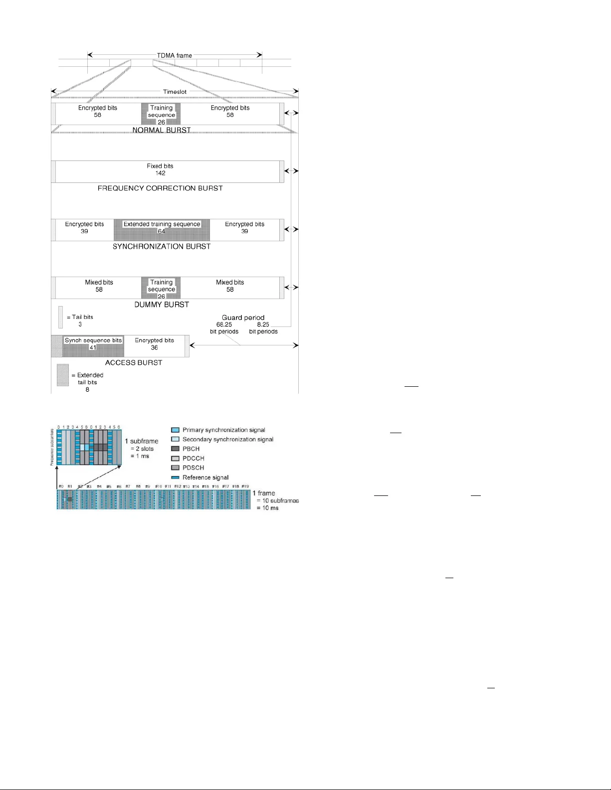
Identification of GSM and L TE Signals Using Their Second-order Cyclostationarity Ebrahim Karami ∗ , Octavia A. Dobre ∗ , and Nikhil Adnani † ∗ Electrical and Computer Engineering, Memorial Univ ersity , Canada email: { ekarami,odobre } @mun.ca † ThinkRF Corp., Ottawa, Canada email: info@thinkrf.com Abstract —A utomatic signal identification (ASI) has v arious mil- litary and commercial applications, such as spectrum surveillance and cognitive radio. In this paper , a novel ASI algorithm is proposed f or the identification of GSM and L TE signals, which is based on the pilot-induced second-order cyclostationarity . The proposed algorithm pr ovides a very good perf ormance at low signal-to-noise ratios and short observation times, with no need for channel estimation, and timing and fr equency synchro- nization. Simulations and off-the-air signals acquired with the ThinkRF WSA4000 receiver are used to confirm the findings. Index T erms —Global system of mobile (GSM), long term evolution (L TE), cyclostationarity . I . I N T RO D U C T I O N Automatic signal identification (ASI) has been initially in- vestigated for military communications, e.g., for electronic warfare and spectrum surv eillance [1]. More recently , ASI has found applications to commercial communications, in the context of software defined and cognitive radios [2], [3]. ASI tackles the problem of identifying the signal type without relying on pre-processing, such as channel estimation, and timing and frequency synchronization [1], [3]–[14]. While most of the ASI w ork in the literature has been done for generic signals, very fe w papers in v estigate the identifica- tion of standard signals; ho wev er , the latter is crucial for spectrum surveillance and cogniti ve radio applications. ASI techniques usually exploit signal features to identify the signal type [1], [4]–[13], and the feature-based identification of standard signals has been carried out as follows. In [4], the authors use second-order cyclostationarity-based features to classify different IEEE 802.11 standard signals. The pilot- induced cyclostationarity of the IEEE 802.11a standard sig- nals is studied in [5], with ASI application. K urtosis-based features are proposed in [6], [7] to identify OFDM-based stan- dard signals. Furthermore, the cyclic prefix (CP)-, preamble-, and reference-signal-induced second-order cyclostationarity of L TE and W iMAX standard signals is exploited in [8]–[11] for This work was supported in part by the National Sciences and Engineering Research Council of Canada (NSERC) through the Engage program. their identification. While the previously mentioned feature- based ASI techniques are dev eloped for orthogonal frequency division multiplexing (OFDM)-based signals, they are not necessarily appropriate to other standard signals, such as GSM. Therefore, to identify such standard cellular signals, we need to develop ASI algorithms based on ne w features. In wireless communications systems, pilot signals are used for channel estimation, as well as frequency and timing synchronization. As the pilot symbols are sent periodically , one can use this periodicity to identify different wireless standard signals. In this paper , we propose a low complexity algorithm to identify the GSM and L TE standard signals, as being widely used in Canada; off-the-air signals are used for verification. The rest of the paper is organized as follo ws. Section II presents the model for the GSM and L TE standard signals. Section III introduces the proposed algorithm for the iden- tification of these signals. In Section IV, results for off-the- air signals acquired with the ThinkRF WSA4000 receiver are shown, along with simulation results. The paper is concluded in Section V. I I . S I G NA L M O D E L In this section, the signal model for the GSM and L TE downlink (DL) is introduced. More specifically , we present the pilot signals in these standards, as their periodicity will be exploited for the identification feature. A. GSM Signal Model The GSM frame structure is sho wn in Fig. 1, including the normal b urst, which carries data, the control bursts, such as frequency correction and synchronization, as well as the access bursts [15]. In the normal burst, 26 bits in each time slot are dedicated to training; these are repeated every time slot and used for channel estimation. Since the duration of each time slot is 577 µ s, the repetition frequency of the pilot sequence is 1733 Hz. From Fig. 1, one can see that the other GSM bursts hav e similar repetitive sequences, but with dif ferent lengths; howe ver , all repeat with the same frequency , i.e., 1733 Hz. Fig. 1. Time slot and format of bursts in the GSM systems [15]. Fig. 2. L TE FDD DL frame structure [17]. B. L TE DL Signal Model The L TE frequency di vision duplex (FDD) DL frame structure is sho wn in Fig. 2. Each L TE frame includes 20 time slots, each with 6 or 7 OFDM symbols, depending if the short or long CP is used [16]. In Canada, L TE with short CP is commonly employed. From Fig. 2, one can see that the samples which are periodically repeated correspond to the cell specific reference signals (RSs), and primary and secondary synchronization channels (PSCH and SSCH), where the RS is repeated e very time slot and PSCH and SSCH are repeated ev ery 10 time slots. The duration of each L TE time slot is 0.5 ms. Consequently , the repetition frequency for the RSs is 2 kHz, while for the PSCH and SSCH is 200 Hz. I I I . P RO P O S E D S I G N AL I D E N T I FI C A T I O N A L G O R I T H M In this section, the algorithm proposed for the identification of GSM and L TE standard signals is presented. First, we introduce the fundamental concept of signal cyclostationarity in order to further discuss the identification feature, and then present the feature-based algorithm and study its complexity . A. Second-or der Signal Cyclostationarity A signal r ( t ) e xhibits second-order cyclostationarity if its first and second-order time-v arying correlation functions are periodic in time [18]. In this work, the following second-order time-varying correlation function is considered c ( t, τ ) = E [ r ( t ) r ∗ ( t + τ )] , (1) where ∗ denotes complex conjugation, E [ . ] is the statistical expectation, and τ is the delay . If c ( t, τ ) is periodic in time with the fundamental period M 0 , then it can be expressed by a Fourier series as [18] c ( t, τ ) = X { α } C ( α , τ ) e j 2 πtα . (2) The Fourier coef ficients defined as C ( α , τ ) = 1 M 0 Z M 0 0 c ( t, τ ) e − j 2 πtα d t, (3) are referred to as the c yclic correlation function (CCF) at cyclic frequency (CF) α and delay τ . The set of CFs is giv en by { α } = { ` M 0 , ` ∈ I , with I as the set of integers } . Assuming M r as the number of received samples, CCF at CF α and delay τ is estimated from the receiv ed sequence, r ( m ) , as [19] ˆ C ( α , τ ) = 1 M r M r − 1 X m =0 r ( m ) r ∗ ( m + τ T s ) e − j 2 παmT s . (4) where T s is the sampling period and τ is multiple integer of T s . Due to the periodicity of the pilot signals in GSM and L TE standards, one can show that these induce second-order cyclostationarity with CFs α i = ` T i , i = GSM, L TE, where T i is the time slot duration of the GSM and L TE standards. The pilot-induced second-order cyclostationarity will be used as an identification feature, as presented in the next sub-section. B. Pr oposed Second-or der Cyclostationarity-based Algorithm W e e xplore the CCF at CF α and zero delay C ( α, 0) to identify the GSM and L TE standard signals, as follo ws. In the first step, ˆ C ( α , 0) is estimated at CFs α i = 1 T i , i = GSM, L TE. In the second step, the estimated CCF magnitude is compared with a threshold, which is set up based on a constant false alarm criterion. The probability of false alarm is defined as the probability of deciding that the standard signal is present when this is not (either an unknown signal or noise is present). An analytical closed form e xpression of the false alarm probability is obtained based on the distrib ution of the CCF magnitude estimate for the unknown signal and noise; in this case, one can simply infer that the CCF magnitude estimate has an asymptotic Rayleigh distribution [19]. Hence, if the CCF for a specific CF α and delay τ is used as a discriminating feature, the probability of false alarm is calculated using the complementary cumulative density function of the Rayleigh distribution as P F = exp( − Γ 2 σ 2 r ) , (5) where σ 2 r is the variance of the recei ved signal. A summary of the proposed algorithm is provided as follo ws. Proposed algorithm Input: The recei ved sequence r ( m ) , m = 0 , ..., M r − 1 . - Estimate the CCF , C i = ˆ C ( α i , 0) , using (4) at CFs α i = 1 T i , i = GSM, L TE. - Estimate the variance of the receiv ed signal, σ 2 r , and calculate the threshold using (5). if C i > Γ then - The receiv ed signal is identified as i , i = GSM, L TE. else - The type of the received signal is not i and it can be either an intruder or noise. end if Computational complexity: W e ev aluate the computational complexity of the proposed identification algorithm through the number of floating point operations (flops) [20], where a complex multiplication and addition require six and two flops, respectiv ely . Based on (4), one can easily see that the number of complex multiplications and additions needed to calculate the CCF equals 2 M r and M r − 1 , respectiv ely . By considering that the thresholding does not require additional complexity , it is straightforward that the number of flops needed by the algorithm equals 14 M r − 2 . It is worth noting that with an av erage Intel Core i750, the identification process takes 68.5 ms for M r = 50000 ; hence, the algorithm can be implemented in practice. I V . R E S U LT S In this section, the results for simulated and of f-the-air signals are presented. A. CCF for Simulated Signals Here we present simulation results for the CCF magnitude of the GSM and L TE signals. For each case, a signal burst of 1000 time slots is generated and then transmitted through a frequenc y-selectiv e fading channel consisting of L p = 4 0 1000 2000 3000 4000 5000 6000 7000 8000 9000 10000 0 0.02 0.04 0.06 0.08 0.1 0.12 0.14 0.16 0.18 0.2 α (Hz) | ˆ C ( α , 0) | Fig. 3. CCF magnitude vs. CF for simulated GSM signals. 0 1000 2000 3000 4000 5000 6000 7000 8000 9000 10000 0 0.05 0.1 0.15 0.2 0.25 0.3 0.35 0.4 0.45 0.5 α (Hz) | ˆ C ( α , 0) | Fig. 4. CCF magnitude vs. CF for simulated L TE signals. statistically independent taps, each being a zero-mean complex Gaussian random variable. The channel is characterized by an e xponential po wer delay profile, σ 2 ( p ) = B h exp ( − p/ 5) , where p = 0 , ..., L p − 1 and B h is chosen such that the av erage power is normalized to unity and SNR is 20 dB. Fig. 3 presents simulation results for the GSM signals, while Fig. 4 shows results for the L TE signals. As expected, one can easily see that the CCF obtained from the simulated GSM signal has peaks at CFs equal to multiple integers of 1733 Hz, which is the reciprocal of the GSM time slot duration. Furthermore, also as expected, the estimated CCF for the simulated L TE signal has peaks at CFs equal to multiple integers of 2 kHz, which is the reciprocal of the L TE time slot duration. B. CCF for Off-the-air Signals In this section, results for the CCF magnitude estimated from the signals receiv ed by a WSA4000 receiver is presented. The location of measurements was the ThinkRF company , in the north Kanata area of Ottawa, Canada. F or each frequency band, 10 6 samples were receiv ed. The bandwidth of the signal recei ved by the WSA4000 receiver was 125 MHz, and the system had a decimation rate parameter to decrease the bandwidth; as such, depending on the expected bandwidth 0 1000 2000 3000 4000 5000 6000 7000 8000 9000 10000 0 0.02 0.04 0.06 0.08 0.1 0.12 0.14 0.16 0.18 0.2 α (Hz) | ˆ C ( α , 0) | Fig. 5. CCF magnitude vs. CF for a signal received by the WSA4000 system within the frequency band of 869 MHz. of the received signal, an appropriate decimation factor was considered. Please note that the proposed algorithm does not need to know the e xact bandwidth of the recei ved signal; as long as the signal of interest is in the bandwidth of the received signal, the proposed algorithm can identify it. Fig. 5 presents the CCF magnitude results for the signal in the 869 MHz band, where we expect the GSM signal from the Rogers base station (BS) located at approximately 460 meter away from our receiver . The decimation factor for this measurement was 64, corresponding to a 1.951 MHz recei ve bandwidth. This bandwidth was enough to co ver the GSM bands supported by the corresponding BS 1 . From Fig. 5, one can see that the CCF estimated from the of f-the-air GSM signal has peaks at CFs equal to multiple inte gers of 1733 Hz, which agrees with the simulation results. Fig. 6 presents the CCF magnitude results for the signal in the 2115 MHz band, where we expect the L TE signal from the Rogers BS located at approximately 460 meter away from the receiv er (the location of this BS is the same as in the previous case). The decimation factor for this measurement was 16, corresponding to a 7.81 MHz receiv e bandwidth, which covers the L TE signal transmitted by the BS. From Fig. 6, one can see that the CCF estimated from the off-the-air L TE signal has peaks at CFs equal to multiple integers of 2 kHz, which concurs with the simulation results. C. P erformance of the Pr oposed Algorithm In this section, the performance of the proposed algorithm for the identification of GSM and L TE signals is ev aluated by Monte Carlo simulation through averaging ov er 1000 iterations. The simulation parameters are the same as in sub- section IV -A. The threshold is set up based on the constant false alarm criterion, and in each iteration, data is generated with a random timing offset taken from a uniform distribution within the first time slot. 1 Each GSM band is 200 kHz. 0 1000 2000 3000 4000 5000 6000 7000 8000 9000 10000 0 0.05 0.1 0.15 0.2 0.25 0.3 0.35 0.4 0.45 0.5 α (Hz) | ˆ C ( α , 0) | Fig. 6. CCF magnitude vs. CF for a signal received by the WSA4000 system within the frequency band of 2115 MHz. −20 −15 −10 −5 0 5 10 15 20 0 0.1 0.2 0.3 0.4 0.5 0.6 0.7 0.8 0.9 1 SNR (dB) P ( λ = ξ | ξ ) , ξ = GSM T = 5 0 msec T = 4 0 msec T = 3 0 msec T = 2 0 msec T = 1 0 msec Fig. 7. Probability of correct identification for the GSM signals, P ( λ = ξ | ξ ) , ξ = GSM, versus SNR for different observ ation times, T . Fig. 7 presents the performance of the proposed algorithm for the identification of the GSM signals for different obser- vation times, with P F = 10 − 2 . From Fig. 7, one can see that with SNR > 0 dB, the probability of correct identification, P ( λ = GSM | GSM ) , approaches one at an observation time as low as 10 ms, while with 50 ms, this occurs at about -5 dB SNR. Fig. 8 presents the performance of the proposed algorithm for the detection of the L TE signals for different observation times, with P F = 10 − 2 . From Fig. 8, one can notice that with SNR > -5 dB, the probability of correct correct identification, P ( λ = L TE | L TE ) , approaches one at an observation time as lo w as 10 ms. In all cases, the results obtained for the L TE signal is better than for the GSM signal; ho wev er , one can obtain a good performance at short observation times and with low SNR for both signal types. Fig. 9 presents the performance of the proposed algorithm for the identification of the GSM and L TE signals for different P F values, with an observation time of T = 10 ms. From Fig. 9, one can see that for L TE signals with SNR > -5 dB, a very −20 −15 −10 −5 0 5 10 15 20 0 0.1 0.2 0.3 0.4 0.5 0.6 0.7 0.8 0.9 1 SNR (dB) P ( λ = ξ | ξ ) , ξ = L T E T = 5 0 msec T = 4 0 msec T = 3 0 msec T = 2 0 msec T = 1 0 msec Fig. 8. Probability of correct identification for the L TE signals, P ( λ = ξ | ξ ) , ξ = L TE, versus SNR for dif ferent observation times, T . −20 −15 −10 −5 0 5 10 15 20 0 0.1 0.2 0.3 0.4 0.5 0.6 0.7 0.8 0.9 1 SNR (dB) P ( λ = ξ | ξ ) , ξ = L TE , GSM P F = 10 − 1 P F = 10 − 2 P F = 10 − 3 ξ =L TE ξ =G SM Fig. 9. Probability of correct identification for the GSM and L TE signals, P ( λ = ξ | ξ ) , ξ = GSM , L TE, versus SNR for dif ferent P F values. Solid lines are used for the L TE signal and dashed lines are used for the GSM signal. good performance is achieved regardless of the P F value; at lower SNRs, it is observed that P ( λ = L TE | L TE ) improv es as P F increases. For the GSM signal, P ( λ = GSM | GSM ) approaches one for SNR > 0 dB regardless of the P F value; at lower SNRs, the performance also enhances as P F increases. In all cases, a better performance is attained for L TE signal identification when compared with GSM. V . C O N C L U S I O N In this paper , we proposed a very low complexity second- order cyclostationarity based algorithm for the identification of the GSM and L TE standard signals, which are commonly used in Canada. The proposed algorithm attains a very good performance at low SNRs and with short observ ation times. Signals acquired by a ThinkRF WSA4000 receiver were used to prov e the concept. A C K N O W L E D G M E N T The authors would like to ackno wledge T im Hember and Dr . T arek Helaly from ThinkRF Corp. for their kind support. R E F E R E N C E S [1] O. A. Dobre, A. Abdi, Y . Bar-Ness, and W . Su, “A Survey of Automatic Modulation Classification T echniques: Classical Approaches and New Dev elopments, ” IET Communications , vol. 1, pp. 137–156, Apr. 2007. [2] J. Mitola and G. Maguire, “Cognitive Radio: Making Software Radios More Personal, ” IEEE P ersonal Communications , v ol. v ol. 6, no. 4, pp. 13–18, Aug. 1999. [3] T . Y ucek and H. Arslan, “A Surve y of Spectrum Sensing Algorithms for Cognitiv e Radio Applications, ” IEEE Communications Surveys and T utorial , vol. 11, no. 1, pp. 116–130, Mar . 2009. [4] K. Kim, C. M. Spooner, I. Akbar, and J. H. Reed, “Specific Emitter Identification for Cognitive Radio with Application to IEEE 802.11, ” in Pr oc. IEEE Global T elecommunications Conference , 2008, pp. 1-5. [5] M. Adrat, J. Leduc, S. Couturier, M. Antweiler , and H. Elders-Boll, “2nd Order Cyclostationarity of OFDM Signals: Impact of Pilot T ones and Cyclic Prefix, ” in Pr oc. IEEE International Confer ence on Commu- nications , 2009, pp. 1-5. [6] A. Bouzegzi, P . Jallon, and P . Ciblat, “A Fourth-order Based Algorithm for Characterization of OFDM Signals, ” in Pr oc. IEEE SP A WC , 2012, pp. 411-415. [7] A. Bouzegzi, P . Ciblat, and P . Jallon, “New Algorithms for Blind Recognition of OFDM Based Systems, ” ELSEVIER: Signal Processing , vol. 90, pp. 900–913, Mar . 2010. [8] A. Al-Habashna, O. A. Dobre, R. V enkatesan, and D. C. Popescu, “W iMAX Signal Detection Algorithm Based on Preamble-induced Second-order Cyclostationarity , ” in Proc. IEEE Global T elecommuni- cations Confer ence , 2010, pp. 1-5. [9] ——, “Cyclostationarity-based Detection of L TE OFDM Signals for Cognitiv e Radio Systems, ” in Pr oc. IEEE Global T elecommunications Confer ence , 2010, pp. 1-6. [10] ——, “Second-Order Cyclostationarity of Mobile W iMAX and L TE OFDM Signals and Application to Spectrum A wareness in Cognitive Radio Systems, ” IEEE Journal of Selected T opics in Signal Processing , vol. 6, no. 1, pp. 26–42, Feb. 2012. [11] ——, “Joint Cyclostationarity-based Detection and Classification of Mobile WiMAX and L TE OFDM Signals, ” in Proc. IEEE International Confer ence on Communications , 2011, pp. 1-6. [12] W . Gardner and C. Spooner, “Signal Interception: Performance Advan- tages of Cyclic-Feature Detectors, ” IEEE T ransactions on Communica- tions , vol. 40, no. 1, pp. 149–159, Jan. 1992. [13] A. Punchihewa, Q. Zhang, O. A. Dobre, C. Spooner , and R. Inkol, “On the Cyclostationarity of OFDM and Single Carrier Linearly Digitally Modulated Signals in Time Dispersiv e Channels: Theoretical Dev elop- ments and Application, ” IEEE T ransactions on W ir eless Communica- tions , vol. 9, pp. 2588–2599, Mar . 2010. [14] W . Su, J. Xu, and M. Zhou, “Real-time Modulation Classification Based On Maximum Likelihood, ” IEEE Communications Letters , vol. vol. 12, no. 11, pp. 801 – 803, Nov . 2008. [15] European T elecommunications Standard Institute (ETSI), Rec. ETSI/GSM 05.02, Multiplexing and Multiple Access on the Radio P ath . version 3.5.1, Mar. 1992. [16] A. Ghosh, J. Zhang, J. Andrews, and R. Muhamed, Fundamentals of LTE . Prentice Hall, 2010. [17] M. Rumney , L TE and the Evolution to 4G W ireless: Design and Measur ement Challenges, 2nd Edition , 2nd ed. W iley , 2013. [18] W . Gardner and C. Spooner, “The Cumulant Theory of Cyclostationary T ime-Series, Part I. Foundation, ” IEEE T ransactions on Signal Pr ocess- ing , vol. 42, no. 12, pp. 3387–3408, Dec. 1994. [19] A. Dandawate and G. Giannakis, “Statistical T ests for Presence of Cyclostationarity , ” IEEE Tr ansactions on Signal Pr ocessing , vol. 42, no. 9, pp. 2355–2369, Sep. 1994. [20] S. W atkins, Fundamentals of Matrix Computations . W iley , 2002.