Approximating the Distribution of the Median and other Robust Estimators on Uncertain Data

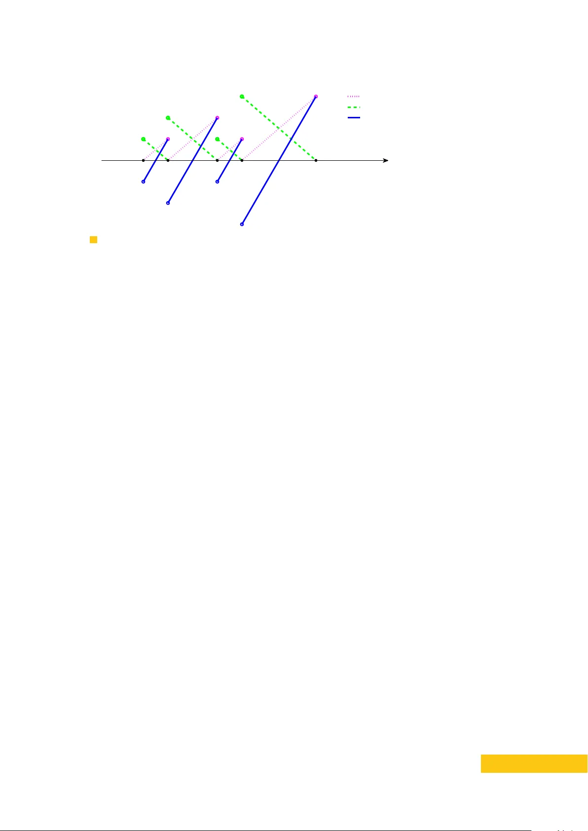
App ro ximating the Distribution of the Median and other Robust Estimato rs on Uncertain Data Kevin Buc hin Departmen t of Mathematics and Computer Science, TU Eindho ven [Eindho v en, The Netherlands] k.a.buc hin@tue.nl h ttps://orcid.org/0000-0002-3022-7877 Jeff M. Phillips Sc ho ol of Computing, Univ e rsit y of Utah [Salt Lak e Cit y , USA] jeffp@cs.utah.edu Pingfan T ang Sc ho ol of Computing, Univ e rsit y of Utah [Salt Lak e Cit y , USA] tang1984@cs.utah.edu Abstract Robust estimators, like the median of a point set, are imp ortant for data analysis in the presence of outliers. W e study robust estimators for lo cationally uncertain points with discrete distributions. That is, each point in a data set has a discrete probabilit y distribution describing its lo cation. The probabilistic nature of uncertain data mak es it c hallenging to compute such estimators, since the true v alue of the estimator is no w describ ed by a distribution rather than a single point. W e sho w how to construct and estimate the distribution of the median of a point set. Building the approximate supp ort of the distribution takes near-linear time, and assigning probabilit y to that support takes quadratic time. W e also develop a general approximation tec hnique for distributions of robust estimators with resp ect to ranges with b ounded V C dimension. This includes the geometric median for high dimensions and the Siegel estimator for linear regression. 2012 A CM Subject Classification Theory of computation ∼ Computational geometry Keyw ords and phrases Uncertain Data, Robust Estimators, Geometric Median, T ukey Median F unding NSF CCF-1115677, CCF-1350888, I IS-1251019, A CI-1443046, CNS-1514520, CNS-1564287, and NW O pro ject no. 612.001.207 1 Intro duction Most statistical or machine learning mo dels of noisy data start with the assumption that a data set is drawn iid (indep endent and identically distributed) from a single distribution. Suc h distributions often represent some true phenomenon under some noisy observ ation. Therefore, approaches that mitigate the influence of noise, inv olving robust statistics or regularization, hav e b ecome commonplace. Ho w ever, many mo dern data sets are clearly not generated iid, rather each data element represen ts a separate ob ject or a region of a more complex phenomenon. F or instance, eac h data element may represent a distinct p erson in a p opulation or an hourly temp erature reading. Y et, this data can still b e noisy; for instance, multiple GPS locational estimates of a p erson, or multiple temp erature sensors in a city . The set of data elemen ts may be noisy and there may b e multiple inconsistent readings of eac h elemen t. T o mo del this noise, the inconsisten t readings can naturally b e interpreted as a probability distribution. XX :2 App roximating the Distribution of the Median on Uncertain Data Giv en such lo cationally noisy , non-iid data sets, there are many unresolved and imp ortant analysis tasks ranging from classification to regression to summarization. In this paper, we initiate the study of robust estimators [ 17 , 26 ] on lo cationally uncertain data. More precisely , w e consider an input data set of size n , where each data p oint’s lo cation is describ ed by a discrete probability distribution. W e will assume these discrete distributions hav e a supp ort of at most k p oin ts in R d ; and for concreteness and simplicity w e will fo cus on cases where eac h p oint has supp ort describ ed by exactly k p oints, eac h b eing equally likely . Although algorithms for lo cationally uncertain p oints hav e b een studied in quite a few con texts ov er the last decade [ 14 , 24 , 20 , 5 , 18 , 4 , 2 , 3 , 34 ] (see more through discussion in full version [ 10 ]), few hav e directly addressed the problem of noise in the data. As the uncertain t y is often the direct consequence of noise in the data collection pro cess, this is a pressing concern. As such we initiate this study fo cusing on the most basic robust estimators: the median for data in R 1 , as well as its generalization the geometric median and the T ukey median for data in R d , defined in Section 1.1. Being robust refers to the fact that the median and geometric medians hav e a br e akdown p oint s of 0.5, that is, if less than 50% of the data p oin ts (the outliers) are mo ved from the true distribution to some lo cation infinitely far aw ay , the estimator remains within the extent of the true distribution [ 25 ]. The T ukey median has a breakdown p oint betw een 1 d +1 and 1 3 [7]. In this pap er, we generalize the median (and other robust estimators) to lo cationally uncertain data, where the outliers can o ccur not just among the n data p oints, but also as part of the discrete distributions representing their p ossible lo cations. The main challenge is in mo deling these robust estimators. As we do not hav e precise lo cations of the data, there is not a single minimizer of cost ( x, Q ) ; rather there ma y b e as man y as k n p ossible input p oint sets Q (the combination of all p ossible lo cations of the data). And the exp ected v alue of such a minimizer is not robust in the same wa y that the mean is not robust. As such we build a distribution ov er the p ossible locations of these cost-minimizers. In R 1 (b y defining boundary cases carefully) this distribution is of size at most O ( nk ) , the size of the input, but already in R 2 it may b e as large as k n . Our Results. W e design algorithms to create an appro ximate supp ort of these median distributions. W e create small sets T (called an ε -supp ort ) such that eac h p ossible median m Q from a p ossible p oin t set Q is within a distance ε · cost ( m Q , Q ) of some x ∈ T . In R w e can create a supp ort set T of size O ( k /ε ) in O ( nk log ( nk )) time. W e show that the b ound O ( k /ε ) is tight since there may b e k large enough mo des of these distributions, each requiring Ω(1 /ε ) p oints to represent. In R d our b ound on | T | is O ( k d /ε d ) , for the T ukey median and the geometric median. If w e do not need to cov er sets of medians m Q whic h o ccur with probabilit y less than ε , we can get a b ound O ( d/ε 2 ) in R d . In fact, this general approach in R d extends to other estimators, including the Siegel estimator [ 28 ] for linear regression. W e then need to map weigh ts onto this support set T . W e can do so exactly in O ( n 2 k ) time in R 1 or approximately in O (1 /ε 2 ) time in R d . Another goal may b e to then construct a single-p oint estimator of these distributions: the median of these median distributions. In R 1 w e can show that this pro cess is stable up to cost ( m Q , Q ) where m Q is the resulting single-p oint estimate. How ever, we also show that already in R 1 suc h estimators are not stable with resp ect to the weigh ts in the median distribution, and hence not stable with resp ect to the probabilit y of any p ossible location of an uncertain point. That is, infinitesimal c hanges to suc h probabilities can greatly change the lo cation of the single-p oint estimator. As such, we argue the approximate median distribution (whic h is stable with resp ect to these changes) is the b est robust represen tation of suc h data. K. Buchin, J. M. Phillips, and P . T ang XX :3 1.1 F ormalization of Mo del and Notation W e consider a set of n lo cationally uncertain p oints P = { P 1 , . . . , P n } so that each P i has k p ossible lo cations { p i, 1 , . . . , p i,k } ⊂ R d . Here, P i = { p i, 1 , . . . , p i,k } is a m ultiset, which means a point in P i ma y app ear more than once. Let P flat = ∪ i { p i, 1 , . . . , p i,k } represen t all p ositions of all p oints in P , which implies P flat is also a multiset. W e consider each p i,j to b e an equally likely (with probability 1 /k ) lo cation of P i , and can extend our techniques to non-uniform probabilities and uncertain p oints with fewer than k p ossible lo cations. F or an uncertain p oint set P w e say Q b P is a tr aversal of P if Q = { q 1 , . . . q n } has each q i in the domain of P i (e.g., q i = p i,j for some j ). W e denote by Pr Q b P [ γ ( Q )] the probabilit y of the even t γ ( Q ) , given that Q is a randomly selected trav ersal from P , where the selection of eac h q i from P i is indep endent of q i 0 from P i 0 . W e are particularly interested in the case where n is large and k is small. F or technical simplicit y we assume an extended RAM mo del where k n (the num b er of p ossible trav ersals of p oint sets) can b e computed in O (1) time and fits in O (1) words of space. W e consider three definitions of medians. In one dimension, given a set Q = { q 1 , q 2 , . . . , q n } that w.l.o.g. satisfies q 1 ≤ q 2 ≤ . . . ≤ q n , we define the me dian m Q as q n +1 2 when n is o dd and q n 2 when n is even. There are several w a ys to generalize the median to higher dimensions [ 7 ], herein we focus on the geometric median and T ukey median. Define cost ( x, Q ) = 1 n P n i =1 k x − q i k where k · k is the Euclidian norm. Giv en a set Q = { q 1 , q 2 , . . . , q n } ⊂ R d , the ge ometric me dian is defined as m Q = arg min x ∈ R d cost ( x, Q ) . The T uk ey depth [ 30 ] of a p oin t p with resp ect to a set Q ⊂ R d is defined depth Q ( p ) := min H ∈H p | H ∩ Q | where H p := { H is a closed half space in R d | p ∈ H } . Then a T ukey me dian of a set Q is a p oint p that can maximize the T ukey depth. 1.2 Related W o rk on Uncertain Data The algorithms and computational geometry communities hav e recently generated a large amoun t of researc h in trying to understand ho w to efficiently pro cess and represent uncertain data [ 14 , 24 , 20 , 5 , 18 , 21 , 4 , 2 , 3 , 1 ], not to mention some motiv ating systems and other progress from the database comm unit y [ 27 , 16 , 15 , 34 , 6 ]. Some work in this area considers other mo dels, with either worst-case representations of the data uncertaint y [ 31 ] which do not naturally allow probabilistic mo dels, or when the data may not exist with some probabilit y [ 18 , 21 , 5 ]. The second mo del can often b e handled as a sp ecial case of the lo cationally uncertain mo del w e study . Among lo cationally uncertain data, most work fo cuses on data structures for easy data access [ 12 , 15 , 29 , 3 ] but not the direct analysis of data. Among the w ork on analysis and summarization, such as for histograms [ 13 ], conv ex h ulls [ 5 ], or clustering [ 14 ] it usually fo cuses on quantities like the exp ected or most likely v alue, which ma y not b e stable with resp ect to noise. This includes estimation of the exp ected median in a stream of uncertain data [ 19 ] or the exp ected geometric median as part of k -median clustering of uncertain data [ 14 ]. W e are not aw are of an y w ork on modeling the probabilistic nature of lo cationally uncertain data to construct robust estimators of that data, robust to outliers in b oth the set of uncertain p oints as well as the probabilit y distribution of each uncertain p oint. 2 Constructing a Single P oint Estimate W e b egin by exploring the construction of a single p oint estimator of set of n lo cationally uncertain p oints P . W e demonstrate that while the estimator is stable with resp ect to the XX :4 App roximating the Distribution of the Median on Uncertain Data v alue of cost , the actual minim um of that function is not stable and provides an incomplete picture for m ultimo dal uncertainties. It is easiest to explore this through a w eighted p oint set X ⊂ R 1 . Giv en a probability distribution defined b y ω : X → [0 , 1] , w e can compute its weigh ted median b y scanning from smallest to largest until the sum of weigh ts reaches 0 . 5 . There are t wo situations whereby we obtain such a discrete weigh ted domain. The first domain is the set T of p ossible lo cations of medians under differen t instantiations of the uncertain p oin ts with weigh ts ˆ w as the probability of those medians b eing realized; see constructions in Section 3.2 and Section 3.5. Let the resulting weigh ted median of ( T , ˆ w ) b e m T . The second domain is simply the set P flat of all p ossible lo cations of P , and its weigh t w where w ( p i,j ) is the fraction of Q b P whic h take p i,j as their median (p ossibly 0 ). Let the w eigh ted median of ( P flat , w ) b e m P . I Theo rem 1. | m T − m P | ≤ ε cost ( m P ) ≤ ε cost ( m Q , Q ) , Q b P is any tr aversal with m P as its me dian. Pro of. W e can divide R in to | T | in terv als, one asso ciated with each x ∈ T , as follows. Each z ∈ R is in an interv al asso ciated with x ∈ T if z is closer to x than any other p oint y ∈ T , unless | z − y | ≤ ε cost ( z ) but | z − x | > cost ( z ) . Th us a point p i,j whose weigh t w ( p i,j ) con tributes to ˆ w ( x ) , is in the in terv al asso ciated with x . Th us, if p i,j = m P , then the sum of all weigh ts of all points greater than p i,j is at most 0 . 5 , and the sum of all weigh ts of p oints less than p i,j is less than 0 . 5 . Hence if m P is in an in terv al asso ciated with x ∈ T , then the sum of all weigh ts of p oints p i,j in interv als greater than that of x m ust b e at most 0 . 5 and those less than that of x m ust b e less than 0 . 5 . Hence m T = x , and | x − p i,j | ≤ ε cost ( m P ) as desired. J Non-Robustness of single p oint estimates. The geometric median of the set { m Q is a geometric median of Q | Q b P } is not stable under small perturbations in w eights; it sta ys within the conv ex hull of the set, but otherwise not muc h can b e said, even in R 1 . Consider the example with n = 3 and k = 2 , where p 1 , 1 = p 1 , 2 = p 2 , 1 = 0 and p 2 , 2 = p 3 , 1 = p 3 , 2 = ∆ for some arbitrary ∆ . The median will b e at 0 or ∆ , eac h with probability 1 / 2 , dep ending on the lo cation of P 2 . W e can also create a more intricate example where ˆ cost (0) = ˆ cost (∆) = 0 . As these examples hav e m Q at 0 or ∆ equally likely with probability 1 / 2 , then canonically in R 1 w e would hav e the median of this distribution at 0 , but a slight change in probability (sa y from sampling) could put it all the wa y at ∆ . This indicates that a represen tation of the distribution of medians as we study in the remainder is more appropriate for noisy data. 3 App roximating the Median Distribution The big c hallenge in constructing an ε -supp ort T is finding the p oints x ∈ P flat whic h hav e small v alues of cost ( x, Q ) (recall cost ( x, Q ) = 1 n P n i =1 k x − q i k ) for some Q b P . But this requires determining the smallest cost Q b P that has x ∈ Q and x is the median of Q . One may think (as the authors initially did) that one could simply use a pro xy function ˆ cost ( x ) = 1 n P n i =1 min 1 ≤ j ≤ k k x − p i,j k , whic h is relatively simple to compute as the low er en v elop e of cost functions for each P i . Clearly ˆ cost ( x ) ≤ cost ( x, Q ) for all Q b P , so a set ˆ T satisfying a similar approximation for ˆ cost will satisfy our goals for cost . Ho wev er, there exist (rather adv ersarial) data sets P where ˆ T w ould require Ω( nk ) p oints; see App endix A. On the other hand, we sho w this is not true for cost . The k ey difference b etw een cost and ˆ cost is that ˆ cost do es not enforce the use of some Q b P of whic h x is a median. That is, that (roughly) half the p oin ts are to the left and half to the right for this Q . K. Buchin, J. M. Phillips, and P . T ang XX :5 −3 −2 −1 0 1 2 3 p i, 0 p i, 1 p i, 2 p i, 3 p i, 4 p L i ( p ) R i ( p ) D i ( p ) Figure 1 The plot of L i ( p ) , R i ( p ) and D i ( p ) . Pro xy functions L , R , and D . W e handle this problem by first introducing tw o families of functions, defined precisely shortly . W e let L i ( x ) (resp. R i ( x ) ) represent the contribution to cost at x from the closest p ossible lo cation p i,j of an uncertain p oint P i to the left (resp. righ t) of x . This allows us to decomp ose the elemen ts of this cost. How ever, it do es not help us to enforce this balance. Hence we in tro duce a third proxy function D i ( x ) = L i ( x ) − R i ( x ) capturing the difference b etw een L i and R i . W e will show that the c hoice of whic h points are used on the left or righ t of x is completely determined b y the D i v alues. In particular, we main tain the D i v alues (for all i ∈ [ n ] ) in sorted order, and use the i with larger D i v alues on the righ t, and smaller D i v alues on the left for the min cost Q b P . T o define L i , R i , and D i , we first assume that P flat and P i for all i ∈ [ n ] are sorted (this w ould take O ( nk log ( nk )) time). Then to simplify definitions we add tw o dummy p oints to eac h P i , and introduce the notation e P i = P i ∪ { p i, 0 , p i,k +1 } and e P = { e P 1 , e P 2 , · · · , e P n } , where p i, 0 = min P flat − n ∆ , p i,k +1 = max P flat + n ∆ , and ∆ = max P flat − min P flat . Thus, ev ery p oin t p ∈ P flat can b e view ed as the median of some trav ersal of e P . Moreo ver, since we put the p i, 0 and p i,k +1 p oin ts far enough out, they will essentially act as p oints at infinity and not affect the rest of our analysis. Next, for p ∈ P flat w e define cost ( p ) = min { cost ( p, Q ) | p is the median of Q and Q b e P } . Th us, if there exists Q b P such that p is the median of Q , then cost ( p ) ≤ cost ( p, Q ) . No w to compute cost and exp edite our analysis, for p ∈ [ min P flat − n ∆ , max P flat + n ∆] , w e define L i ( p ) = min {| p i − p | | p i ∈ e P i ∩ ( −∞ , p ] } and R i ( p ) = min {| p i − p | | p i ∈ e P i ∩ [ p, ∞ ) } . and recall D i ( p ) = L i ( p ) − R i ( p ) . Ob viously , if p ∈ e P i , then D i ( p ) = L i ( p ) = R i ( p ) = 0 . F or example, if e P i = { p i, 0 , p i, 1 , p i, 2 , p i, 3 , p i, 4 } and p i, 0 < p i, 1 < p i, 2 < p i, 3 < p i, 4 , then the plot of L i ( p ) , R i ( p ) and D i ( p ) , is sho wn in Figure 1. F or the sake of brevity , we no w assume n is o dd; adjusting a few arguments b y +1 will adjust for the n is even case. Consider next the following prop erty of the D i functions with resp ect to computing cost ( p ) for a point p ∈ P i 0 . Let { i 1 , i 2 , · · · , i n − 1 } = [ n ] \{ i 0 } b e a p ermutation of uncertain p oin ts, except for i 0 , so that D i 1 ( p ) ≤ D i 2 ( p ) ≤ · · · ≤ D i n − 1 ( p ) . Then to minimize cost ( p, Q ) , we coun t the uncertain p oints P i l using L i l if in the p ermutation i l ≤ ( n − 1) / 2 and otherwise coun t it on the right with R i l . This holds since for any other p ermutation XX :6 App roximating the Distribution of the Median on Uncertain Data { j 1 , j 2 , · · · , j n − 1 } = [ n ] \{ i 0 } we hav e P n − 1 l = n +1 2 D i l ( p ) ≥ P n − 1 l = n +1 2 D j l ( p ) and th us n − 1 2 X l =1 L i l ( p ) + n − 1 X l = n +1 2 R i l ( p ) = n − 1 X l =1 L i l ( p ) − n − 1 X l = n +1 2 D i l ( p ) ≤ n − 1 X l =1 L j l ( p ) − n − 1 X l = n +1 2 D j l ( p ) = n − 1 2 X l =1 L j l ( p ) + n − 1 X l = n +1 2 R j l ( p ) . F or p ∈ P i 0 , cost ( p ) = 1 n  P n − 1 2 l =1 L i l ( p ) + P n − 1 l = n +1 2 R i l ( p )  under this D i -sorted p ermutation. 3.1 Computing cost No w to compute cost for all p oints p ∈ P flat , we simply need to maintain the D i in sorted order, and then sum the appropriate terms from L i and R i . Let us first examine a few facts ab out the complexit y of these functions. The function L i (resp. R i ) is piecewise-linear, where the slope is alwa ys 1 (resp. − 1 ). The breakp oin ts only o ccur at x = p i,j for each p i,j ∈ P i . Hence, they each ha ve complexity Θ( k ) for all i ∈ [ n ] . The structure of L i and R i implies that D i is also piecewise-linear, where the slop e is alw a ys 2 and has breakp oints for each p i,j ∈ P i . Each linear comp onent attains a v alue D i ( x ) = 0 when x is the midp oint b etw een t wo p i,j , p i,j 0 ∈ P i whic h are consecutive in the sorted order of P i . The fact that all D i ha v e slop e 2 at all non-discon tinuous p oin ts, and these discontin uous p oin ts only o ccur at P i , implies that the sorted order of the D i functions do es not c hange in b etw een p oints of P flat . Moreov er, at one of these p oints of discontin uity x ∈ P flat , the ordering b etw een D i s only changes for uncertain p oints D i 0 suc h that there exists a p ossible lo cation p i 0 ,j ∈ P i 0 suc h that x = p i 0 ,j . This implies that to maintain the sorted order of D i for any x , as we increase the v alue of x , w e only need to up date this order at the nk p oin ts in P flat with resp ect to D i 0 for which there exists p i 0 ,j ∈ P i 0 with p i 0 ,j = x . This takes O ( log ( nk )) time p er up date using a balanced BST, and thu s O ( nk log ( nk )) time to define cost ( x ) for all v alues x ∈ R 1 . T o compute cost ( x ) , we also require the v alues of L i (or R i ); these can be constructed indep endently for each i ∈ [ n ] in O ( k ) time after sorting, and in O ( nk log k ) time ov erall. 1 Ultimately , we arriv e at the following theorem. I Theorem 2. Consider a set of n unc ertain p oints P with k p ossible lo c ations e ach. W e c an c ompute cost ( x ) for al l x ∈ R such that x = p i,j for some p i,j ∈ P flat in O ( nk log ( nk )) time. 3.2 Building the ε -Supp o rt T and Bounding its Size W e next sho w that there alwa ys exists an ε -supp ort T and it has a size | T | = O ( k ε ) . I Theorem 3. Given a set of n unc ertain p oints P = { P 1 , · · · , P n } , wher e P i = { p i, 1 , · · · , p i,k } ⊂ R , and ε ∈ (0 , 1] we c an c onstruct an ε -supp ort T that has a size | T | = O ( k ε ) . 1 When multiple distinct p i,j coincide at a point x , then more care may b e required to compute cost ( x ) (depending on the specifics of how the median is defined in these boundary cases). Sp ecifically , w e may not wan t to set L i ( x ) = 0 , instead it may b e b etter to use the v alue R i ( x ) even if R i ( x ) = α > 0 . This is the case when α < R i 0 ( x ) − L i 0 ( x ) for some other uncertain p oin t P i 0 (then we say P i is on the right, and P i is on the left). This can be resolv ed by either tw eaking the definition of median for these cases, or sorting all D i ( x ) for uncertain points P i with some p i,j = x , and some b o okkeeping. K. Buchin, J. M. Phillips, and P . T ang XX :7 Pro of. W e first sort P flat in ascending order, scan P flat = { p 1 , · · · , p nk } from left to righ t and c ho ose one p oint from P flat ev ery b n 3 c p oin ts, and then put the chosen point into T . Now, supp ose p is the median of some trav ersal Q b P and cost ( p ) = cost ( p, Q ) . If p / ∈ T , then there are tw o consecutive p oints t, t 0 in T suc h that t < p < t 0 . On either side of p there are at least b n 2 c p oin ts in Q , so without loss of generality , we assume | p − t 0 | ≥ 1 2 | t − t 0 | . Since | [ p, ∞ ) ∩ Q | ≥ n 2 and there are at most b n 3 c p oin ts in [ p, t 0 ] , we hav e | ( t 0 , ∞ ) ∩ Q | ≥ n 2 − b n 3 c ≥ n 6 , whic h implies cost ( p ) = cost ( p, Q ) ≥ 1 n X q ∈ ( t 0 , ∞ ) ∩ Q | q − p | ≥ 1 n X q ∈ ( t 0 , ∞ ) ∩ Q | t 0 − p | ≥ 1 n n 6 | t 0 − p | = 1 6 | t 0 − p | ≥ 1 12 | t − t 0 | . (1) F or any fixed ε ∈ (0 , 1] , and tw o consecutiv e p oints t, t 0 ( t < t 0 ) in T , we put x 1 , · · · , x d 12 ε e− 1 in to T where x i = t + | t − t 0 | i d 12 ε e for 1 ≤ i ≤ d 12 ε e − 1 . So, for the median p ∈ ( t, t 0 ) , there exists x i ∈ T s.t. | p − x i | ≤ ε 12 | t − t 0 | , and from (1) , we kno w | p − x i | ≤ ε cost ( p ) . In total we put O ( k ε ) p oints into T ; thus the pro of is completed. J I Rema rk 1. The ab ov e construction results in an ε -supp ort T of size O ( k /ε ) , but do es not restrict that T ⊂ P flat . W e can enforce this restriction by for eac h x placed in T to choose the single nearest p oint p ∈ P flat to replace it in T . This results in an (2 ε ) -supp ort, which can b e made an ε -supp ort by instead adding d 24 ε e − 1 p oints betw een eac h pair ( t, t 0 ) , without affecting the asymptotic time b ound. I Rema rk 2. W e can construct a sequence of uncertain data { P ( n, k ) } suc h that, for eac h uncertain data P ( n, k ) , the optimal ε -supp ort T has a size Ω( k ε ) . F or example, for ε = 1 3 , 1 5 , 1 7 , · · · , w e define n = 1 ε , and p i,j = ( j − 1) n + i for i ∈ [ n ] and j ∈ [ k ] . Then, for any median p ∈ P flat , we hav e ε cost ( p ) = 2 n 2 P n − 1 2 i =1 i = n 2 − 1 4 n 2 < 1 4 , hence cov ering no other p oints, whic h implies | T | = Ω( nk ) = Ω( k ε ) . W e can construct the minimal size ε -supp ort T in O ( nk log ( nk )) time b y sorting, and greedily adding the smallest p oin t not yet co vered eac h step. This yields the slightly stronger corollary of Theorem 3. I Co rolla ry 4. Consider a set of n unc ertain p oints P = { P 1 , · · · , P n } , wher e P i = { p i, 1 , · · · , p i,k } ⊂ R , and ε ∈ (0 , 1] . W e c an c onstruct an ε -supp ort T in O ( nk log ( nk )) time which has the minimal size for any ε -supp ort, and | T | = O ( k ε ) . There are m ultiple wa ys to generalize the notion of a median to higher dimensions [ 7 ]. W e fo cus on tw o v ariants: the T ukey median and the geometric median. W e start with generalizing the notion of an ε -supp ort to a T ukey median since it more directly follo ws from the techniques in Theorem 3, and then address the geometric median. 3.3 An ε -Supp o rt fo r the T uk ey Median A closely related concept to the T ukey median is a c enterp oint , whic h is a p oin t p suc h that depth Q ( p ) ≥ 1 d +1 | Q | . Since for any finite set Q ∈ R d its centerpoint alw ays exists, a T ukey median m ust b e a cen terp oin t. This means if p is the T ukey median of Q , then for any closed half space containing p , it contains at least 1 d +1 | Q | p oin ts of Q . Using this prop erty , w e can pro v e the follo wing theorem. XX :8 App roximating the Distribution of the Median on Uncertain Data I Theorem 5. Given a set of n unc ertain p oints P = { P 1 , · · · , P n } , wher e P i = { p i, 1 , · · · , p i,k } ⊂ R 2 , and ε ∈ (0 , 1] , we c an c onstruct an ε -supp ort T for the T ukey me dian on P that has a size | T | = O ( k 2 ε 2 ) . Pro of. Supp ose the pro jections of P flat on x -axis and y -axis are X and Y resp ectiv ely . W e sort all p oints in X and choose one p oin t from X ev ery b n 4 c p oin ts, and then put the chosen p oin ts into a set X T . F or each p oint x ∈ X T w e draw a line through ( x, 0) parallel to y -axis. Similarly , we sort all p oin ts in Y and choose one p oint every b n 4 c p oin ts, and put the c hosen p oin ts into Y T . F or each point y ∈ Y T w e draw a line through (0 , y ) parallel to x -axis. No w, supp ose p with co ordinates ( x p , y p ) is the T uk ey median of some trav ersal Q b P and cost ( p, Q ) = 1 n P q ∈ Q k q − p k . If x p / ∈ X T and y p / ∈ Y T , then there are x, x 0 ∈ X T and y , y 0 ∈ Y T suc h that x < x p < x 0 and y < y p < y 0 , as sho wn in Figure 2(a). Without loss of generality , w e assume | x p − x | ≥ 1 2 | x 0 − x | and | y p − y | ≥ 1 2 | y − y 0 | . Since p is the T ukey median of Q , we ha v e | Q ∩ ( −∞ , ∞ ) × ( −∞ , y p ] | ≥ n 3 where ( −∞ , ∞ ) × ( −∞ , y p ] = { ( x, y ) ∈ R 2 | y ≤ y p } . Recall there are at most b n 4 c p oin ts of P flat in ( −∞ , ∞ ) × [ y p , y ] , which implies | Q ∩ ( −∞ , ∞ ) × ( −∞ , y ) | ≥ n 3 − b n 4 c ≥ n 12 . So, we ha ve cost ( p, Q ) ≥ 1 n X q ∈ Q ∩ ( −∞ , ∞ ) × ( −∞ ,y ) k q − p k ≥ 1 n n 12 | y − y p | ≥ 1 24 | y − y 0 | . Using a symmetric argument, we can obtain cost ( p, Q ) ≥ 1 24 | x − x 0 | . F or any fixed ε ∈ (0 , 1] , and any tw o consecutive p oints x, x 0 in X T w e put x 1 , · · · , x d 48 ε e− 1 in to X T where x i = x + | x − x 0 | i d 48 ε e . Also, for any tw o consecutive p oin t y , y 0 in Y T , w e put y 1 , · · · , y d 48 ε e− 1 in to Y T where y i = y + | y − y 0 | i d 48 ε e . So, for the T ukey median p ∈ ( x, x 0 ) × ( y , y 0 ) , there exist x i ∈ X T and y j ∈ Y T suc h that | x p − x i | ≤ ε 48 | x − x 0 | and | y p − y j | ≤ ε 48 | y − y 0 | . Since w e hav e shown that 1 24 | x − x 0 | and 1 24 | y − y 0 | are lo wer b ounds for cost ( p, Q ) , w e obtain k ( x p , y p ) − ( x i , y j ) k ≤| x p − x i | + | y p − y j | ≤ ε 48 ( | x − x 0 | + | y − y 0 | ) ≤ ε 48 (24 cost ( p, Q ) + 24 cost ( p, Q )) = ε cost ( p, Q ) . Finally , we define T as T := X T × Y T . Then for any Q b P , if p is the T uk ey median of Q , there exists t ∈ T suc h that k t − p k ≤ ε cost ( p, Q ) . Thus, T is an ε -supp ort for the T uk ey median on P . Moreo ver, since | X T | = O ( k ε ) and | Y T | = O ( k ε ) , we hav e | T | = O ( k 2 ε 2 ) . J In a straight-forw ard extension, w e can generalize the result of Theorem 5 to d dimensions. I Theorem 6. Given a set of n unc ertain p oints P = { P 1 , · · · , P n } , wher e P i = { p i, 1 , · · · , p i,k } ⊂ R d , and ε ∈ (0 , 1] , we c an c onstruct an ε -supp ort T for the T ukey me dian on P that has a size | T | = O ((2 d ( d + 1)( d + 2) 2 k ε ) d ) . 3.4 An ε -Supp o rt fo r the Geometric Median Unlik e the T ukey median, there does not exist a constant C > 0 suc h that: for any geometric median p of p oint set Q ⊂ R d , any closed half space containing p con tains at least 1 C | Q | p oin ts of Q . F or example, suppose in R 2 there are 2 n + 1 points on x -axis with the median p oin t at the origin; this p oint is also the geometric median. If we mo ve this p oint up w ard along the y direction, then the geometric median also mov es up w ards. Ho wev er, for the line through the new geometric median and parallel to the x -axis, all 2 n other p oints are under this line. K. Buchin, J. M. Phillips, and P . T ang XX :9 Hence, we need a new idea to adapt the metho d in Theorem 6 for the geometric median in R d . W e first consider the geometric median in R 2 . W e show we can find some line through it, such that on b oth sides of this line there are at least n 8 p oin ts. I Lemma 7. Supp ose p is the ge ometric me dian of Q ⊂ R 2 with size | Q | = n . Ther e is a line ` thr ough p so b oth close d half planes with ` as b oundary c ontain at le ast n 8 p oints of Q . Pro of. W e first build a rectangular coordinate system at the point p , which means p is the origin with co ordinates ( x p , y p ) = (0 , 0) . Then we use the x -axis, y -axis and lines x = y , x = − y to decompose the plane into eight regions, as shown in Figure 2(b). Since all these eigh t regions ha v e the same shap e, without loss of generality , w e can assume Ω = { ( x, y ) ∈ R 2 | x ≥ y ≥ 0 } con tains the most p oints of Q . Then | Ω ∩ Q | ≥ n 8 , otherwise n = | Q | = | R 2 ∩ Q | ≤ 8 | Ω ∩ Q | < n , whic h is a contradiction. If | Q ∩ { p }| ≥ n 8 , i.e., the multiset Q con tains p at least n 8 times, then obviously this prop osition is correct. So, w e only need to consider the case | Q ∩ { p }| < n 8 . W e introduce notations e Ω = Ω \ { p } and Ω o = Ω \ ∂ Ω , and denote the co ordinates of an y q ∈ Q as q = ( x q , y q ) . F rom a property of the geometric median (prov en in App endix 14) we know P q ∈ Q \{ p } x q − x p k q − p k ≤ | Q ∩ { p }| . Since | Q ∩ { p }| < n 8 this implies X q ∈ Q ∩ e Ω x q k q k + X q ∈ Q \ Ω x q k q k < n 8 , since p is the origin and Q \ { p } = ( Q ∩ e Ω ) ∪ ( Q \ Ω) . F rom x q k q k = x q √ x 2 q + y 2 q ≥ 1 √ 2 , ∀ q ∈ e Ω w e obtain | Q ∩ e Ω | 1 √ 2 ≤ X q ∈ Q ∩ e Ω x q k q k < n 8 − X q ∈ Q \ Ω x q k q k ≤ n 8 + | Q \ Ω | ≤ n 8 + ( n − | Q ∩ e Ω | ) whic h implies there are not to o man y p oints in e Ω , | Q ∩ e Ω | < √ 2 n (1 + √ 2) · 9 8 < 0 . 66 n. No w, we define the tw o pairs of half spaces which share a b oundary with e Ω : H + 1 = { ( x, y ) ∈ R 2 | y ≥ 0 } , H − 1 = { ( x, y ) ∈ R 2 | y ≤ 0 } and H + 2 = { ( x, y ) ∈ R 2 | x − y ≥ 0 } , H − 2 = { ( x, y ) ∈ R 2 | x − y ≤ 0 } . W e assert either | H + 1 ∩ Q | ≥ n 8 and | H − 1 ∩ Q | ≥ n 8 , or | H + 2 ∩ Q | ≥ n 8 and | H − 2 ∩ Q | ≥ n 8 . Otherwise, since | Q ∩ Ω | ≥ n 8 and Ω ⊂ H + 1 ∩ H + 2 , we hav e p x x ′ x p y y ′ y p p x x ′ x p y y ′ y p θ (a) (b) (c) Figure 2 (a) T uk ey median p is in a grid cell formed by x, x 0 and y , y 0 . (b) The plane is decomp osed into 8 regions with the same shape. (c) Geometric median p is in an oblique grid cell formed b y x, x 0 and y, y 0 . XX :10 App roximating the Distribution of the Median on Uncertain Data | H − 1 ∩ Q | < n 8 and | H − 2 ∩ Q | < n 8 . F rom H − 1 ∪ H − 2 ∪ Ω o = R 2 w e hav e n = | Q | = | R 2 ∩ Q | = | ( H − 1 ∪ H − 2 ∪ Ω o ) ∩ Q | ≤ | H − 1 ∩ Q | + | H − 2 ∩ Q | + | Ω o ∩ Q | ≤| H − 1 ∩ Q | + | H − 2 ∩ Q | + | e Ω ∩ Q | ≤ n 8 + n 8 + 0 . 66 n < n, whic h is a con tradiction. Therefore, among lines ` 1 : y = 0 and ` 2 : x − y = 0 , whic h b oth go through p , one of them has at least n/ 8 p oints from Q on both sides. J I Theorem 8. Given a set of n unc ertain p oints P = { P 1 , · · · , P n } , wher e P i = { p i, 1 , · · · , p i,k } ⊂ R 2 , and ε ∈ (0 , 1] , we c an c onstruct an ε -supp ort T for the ge ometric me dian on P that has a size | T | = O ( k 2 ε 2 ) . Pro of. The idea to prov e this theorem is to use sev eral oblique coordinate systems. W e consider an oblique co ordinate system, the angle b etw een x -axis and y -axis is θ ∈ (0 , π 2 ] , and use the technique in Theorem 5 to generate a grid. More precisely , we pro ject P flat on to the x -axis along the y -axis of the oblique co ordinate system to obtain a set X , sort all points in X , and choose one p oint from X ev ery b n 9 c p oin ts to form a set X T . Then we use the same metho d to generate Y and Y T pro jecting along the x -axis in the oblique co ordinate system. F or each p oint x ∈ X T w e draw a line through ( x, 0) parallel to the (oblique) y -axis, and for eac h p oint y ∈ Y T w e draw a line through (0 , y ) parallel to the (oblique) x -axis. Let p with co ordinates ( x p , y p ) b e the geometric median of some trav ersal Q b P and cost ( p, Q ) = 1 n P q ∈ Q k q − p k . If x p / ∈ X T and y p / ∈ Y T , then there are x, x 0 ∈ X T and y , y 0 ∈ Y T suc h that x p ∈ ( x, x 0 ) and y p ∈ ( y , y 0 ) , as sho wn in Figure 2(c). If we hav e the condition: | Q ∩ ( −∞ , ∞ ) × ( −∞ , y p ] | ≥ n 8 , | Q ∩ ( −∞ , ∞ ) × [ y p , ∞ ) | ≥ n 8 , | Q ∩ ( −∞ , x p ] × ( −∞ , ∞ ) | ≥ n 8 , | Q ∩ [ x p , ∞ ) × ( −∞ , ∞ ) | ≥ n 8 , (2) then we can make the following computation. Without loss of generalit y , w e assume | x p − x | ≥ 1 2 | x 0 − x | and | y p − y | ≥ 1 2 | y − y 0 | . There are at most b n 9 c p oin ts of P flat in ( −∞ , ∞ ) × [ y p , y ] , which implies | Q ∩ ( −∞ , ∞ ) × ( −∞ , y ) | ≥ n 8 − b n 9 c ≥ n 72 . So, we ha ve cost ( p, Q ) ≥ 1 n X q ∈ Q ∩ ( −∞ , ∞ ) × ( −∞ ,y ) k q − p k ≥ 1 n n 72 | y − y p | ≥ sin( θ ) 144 | y − y 0 | . Similarly , we can prov e cost ( p, Q ) ≥ sin( θ ) 144 | x − x 0 | . F or any fixed ε ∈ (0 , 1] , and any t wo consecutiv e p oints x, x 0 in X T w e put x 1 , · · · , x d 288 ε sin( θ ) e− 1 in to X T where x i = x + | x − x 0 | i d 288 ε sin( θ ) e . Also, for an y tw o consecutive p oin t y , y 0 in Y T , we put y 1 , · · · , y d 288 ε sin( θ ) e− 1 in to Y T where y i = y + | y − y 0 | i d 288 ε sin( θ ) e . So, for the L 1 median p ∈ ( x, x 0 ) × ( y , y 0 ) , there exist x i ∈ X T and y j ∈ Y T suc h that | x p − x i | ≤ ε sin( θ ) 288 | x − x 0 | and | y p − y j | ≤ ε sin( θ ) 288 | y − y 0 | . Since we ha v e sho wn that b oth sin( θ ) 144 | x − x 0 | and sin( θ ) 144 | y − y 0 | are low er b ounds for cost ( p, Q ) , using the distance formula in an oblique co ordinate system, we hav e k ( x p , y p ) − ( x i , y j ) k ≤ (( x p − x i ) 2 + ( y p − y j ) 2 + 2( x p − x i )( y i − y p ) cos( θ )) 1 2 ≤ (( x p − x i ) 2 + ( y p − y j ) 2 + 2 | x p − x i || y i − y p | ) 1 2 = | x p − x i | + | y p − y j | ≤ ε sin( θ ) 288 ( | x − x 0 | + | y − y 0 | ) ≤ ε sin( θ ) 288  144 sin( θ ) cost ( p, Q ) + 144 sin( θ ) cost ( p, Q )  = ε cost ( p, Q ) . K. Buchin, J. M. Phillips, and P . T ang XX :11 Therefore, if all k n geometric medians of trav ersals satisfy (2) and θ ∈ (0 , π 2 ] is a constant then T = X T × Y T is an ε -supp ort of size O  k 2 (sin( θ ) ε ) 2  for the geometric median on P . Although we cannot find an oblique co ordinate system to make (2) hold for all k n medians, w e can use several oblique co ordinate systems. Using the result of Lemma 7, for an y geometric median of n p oin ts Q , we know there exists a line ` through p and parallel to a line in { ` 1 : y = 0 , ` 2 : x − y = 0 , ` 3 : x = 0 , ` 4 : x + y = 0 } , such that in b oth sides of this line, there are at least n 8 p oin ts of Q . Since w e did not make any assumption on the distribution of p oin ts in Q , if we rotate ` 1 , ` 2 , ` 3 , ` 4 an ticlo c kwise by π 8 around the origin, we can obtain four lines ` 0 1 , ` 0 2 , ` 0 3 , ` 0 4 , and there exists a line ` 0 through p and parallel to a line in { ` 0 1 , ` 0 2 , ` 0 3 , ` 0 4 } , suc h that on both sides of this line, there are at least n 8 p oin ts of Q . The angle b etw een ` and ` 0 is at least π 8 . Therefore, given L = { ` 1 , ` 2 , ` 3 , ` 4 } and L 0 = { ` 0 1 , ` 0 2 , ` 0 3 , ` 0 4 } , for eac h pair ( `, ` 0 ) ∈ L × L 0 , w e take ` and ` 0 as x -axis and y -axis resp ectively to build an oblique coordinate system, and then use the ab ov e metho d to compute a set T ( `, ` 0 ) . Since for an y geometric median p there m ust b e an oblique co ordinate system based on some ( `, ` 0 ) ∈ L × L 0 to make (2) hold for p , w e can tak e T = ∪ ` ∈ L ,` 0 ∈ L 0 T ( `, ` 0 ) as an ε -supp ort for geometric median on P , and the size of T is | T | = O  16 k 2 (sin( π 8 ) ε ) 2  = O  k 2 ε 2  . J The result of Theorem 8 can b e generalized to R d and details are in App endix C. 3.5 Assigning a Weight to T in R 1 Here we pro vide an algorithm to assign a weigh t to T in R 1 , whic h appro ximates the probabilit y distribution of median. F or T in R d , we provide a randomized algorithm in Section 4.1. Define the w eigh t of p i,j ∈ P flat as w ( p i,j ) = 1 k n |{ Q b P | p i,j is the median of Q }| , the probabilit y it is the median. Suppose T is constructed b y our greedy algorithm for R 1 . F or p i,j ∈ P flat , we introduce a map f T : P flat → T , f T ( p i,j ) = arg min {| x − p i,j | | x ∈ T , | x − p i,j | ≤ ε cost ( p i,j ) } , where cost ( p i,j ) = min { cost ( p i,j , Q ) | p i,j is the median of Q and Q b P } . In tuitiv ely , this maps each p i,j ∈ P flat on to the closest p oint x ∈ T , unless it violates the ε -appro ximation prop erty which another further p oint satisfies. No w for each x ∈ T , define weigh t of x as ˆ w ( x ) = P { p i,j ∈ P flat | f T ( p i,j )= x } w ( p i,j ) . So we first compute the weigh t of each p oint in P flat and then obtain the weigh t of p oints in T in another linear sweep. Our ability to calculate the weigh ts w for each p oin t in P flat is summarized in the next lemma. The algorithm, explained within the pro of, is a dynamic program that expands a sp ecific p olynomial similar to Li et.al. [ 22 ], where in the final state, the co efficients corresp ond with the probability of eac h p oint being the median. I Lemma 9. W e c an output w ( p i,j ) for al l p oints in P flat in R 1 in O ( n 2 k ) time. Pro of. F or an y p i 0 ∈ P i 0 , we define the following terms to count the num b er of p oints to the left ( l j ) or righ t ( r j ) of it in the j th uncertain p oint (excluding P i 0 ): l j = ( |{ p ∈ P j | p ≤ p i 0 }| if 1 ≤ j ≤ i 0 − 1 |{ p ∈ P j +1 | p ≤ p i 0 }| if i 0 ≤ j ≤ n − 1 , r j = ( |{ p ∈ P j | p ≥ p i 0 }| if 1 ≤ j ≤ i 0 − 1 |{ p ∈ P j +1 | p ≥ p i 0 }| if i 0 ≤ j ≤ n − 1 . XX :12 App roximating the Distribution of the Median on Uncertain Data Then, if n is o dd, we can write the weigh t of p i 0 as w ( p i 0 ) = 1 k n X S 1 ∩ S 2 = ∅ S 1 ∪ S 2 = { 1 , ··· ,n − 1 } ( l i 1 · l i 2 · . . . · l i n − 1 2 · r j 1 · r j 2 · . . . · r j n − 1 2 ) , where S 1 = { i 1 , i 2 , · · · , i n − 1 2 } and S 2 = { j 1 , j 2 , · · · , j n − 1 2 } . This sums o ver all partitions S 1 , S 2 of uncertain p oints on the left or right of p i 0 for whic h it is the median, and each term is the pro duct of wa ys each uncertain p oint can b e on the appropriate side. W e define w ( p i 0 ) similarly when n is ev en, then the last index of S 2 is j n 2 . W e next describ e the algorithm for n o dd; the case for n ev en is similar. T o compute P S 1 ∩ S 2 = ∅ S 1 ∪ S 2 = { 1 , ··· ,n − 1 } ( l i 1 · l i 2 · . . . · l i n − 1 2 · r j 1 · r j 2 · . . . · r j n − 1 2 ) , we consider the follo wing p olynomial: ( l 1 x + r 1 )( l 2 x + r 2 ) · · · ( l n − 1 x + r n − 1 ) , (3) where P S 1 ∩ S 2 = ∅ S 1 ∪ S 2 = { 1 , ··· ,n − 1 } ( l i 1 · l i 2 · . . . · l i n − 1 2 · r j 1 · r j 2 · . . . · r j n − 1 2 ) is the co efficient of x n − 1 2 . W e define ρ i,j (1 ≤ i ≤ n − 1 , 0 ≤ j ≤ i ) as the coefficient of x j in the p olynomial ( l 1 x + r 1 ) · · · ( l i x + r i ) and then it is easy to c heck ρ i,j = l i ρ i − 1 ,j − 1 + r i ρ i − 1 ,j . Th us we can use dynamic programming to compute ρ n − 1 , 0 , ρ n − 1 , 1 , · · · , ρ n − 1 ,n − 1 , as shown in Algorithm 1. Algorithm 1 Compute ρ n − 1 , 0 , ρ n − 1 , 1 , · · · , ρ n − 1 ,n − 1 Let ρ 1 , 0 = r 1 , ρ 1 , 1 = l 1 , ρ 1 , 2 = 0 . for i = 2 to n − 1 do for j = 0 to i do ρ i,j = l i ρ i − 1 ,j − 1 + r i ρ i − 1 ,j ρ i,i +1 = 0 return ρ n − 1 , 0 , ρ n − 1 , 1 , · · · , ρ n − 1 ,n − 1 . Th us Algorithm 1 computes the w eigh t 1 k n w ( p i 0 ) = ρ n − 1 , n − 1 2 for a single p i 0 ∈ P flat . Next w e show, we can reuse muc h of the structure to compute the weigh t for another p oin t; this will ultimately sha v e a factor n off of running Algorithm 1 nk times. Supp ose for p i 0 ∈ P i 0 w e hav e obtained ρ n − 1 , 0 , ρ n − 1 , 1 , . . . , ρ n − 1 ,n − 1 b y Algorithm 1, and then we consider p i 0 0 = min { p ∈ P flat \ P i 0 | p ≥ p i 0 } . W e assume p i 0 0 ∈ P i 0 0 , and if i 0 0 < i 0 , we construct a p olynomial ( l 1 x + r 1 ) · · · ( l i 0 0 − 1 x + r i 0 0 − 1 )( ˜ l i 0 0 x + ˜ r i 0 0 )( l i 0 0 +1 x + r i 0 0 +1 ) · · · ( l n − 1 x + r n − 1 ) (4) and if i 0 0 > i 0 , we construct a p olynomial ( l 1 x + r 1 ) · · · ( l i 0 0 − 2 x + r i 0 0 − 2 )( ˜ l i 0 0 − 1 x + ˜ r i 0 0 − 1 )( l i 0 0 x + r i 0 0 ) · · · ( l n − 1 x + r n − 1 ) (5) where ˜ l i 0 0 = ˜ l i 0 0 − 1 = |{ p ∈ P i 0 | p ≤ p i 0 0 }| and ˜ r i 0 0 = ˜ r i 0 0 − 1 = |{ p ∈ P i 0 | p ≥ p i 0 0 }| . Since (3) and (4) ha v e only one differen t factor, w e obtain the co efficien ts of (4) from the co efficients of (3) in O ( n ) time. W e recov er the coefficients of ( l 1 x + r 1 ) · · · ( l i 0 − 1 x + r i 0 − 1 )( l i 0 0 +1 x + r i 0 0 +1 ) · · · ( l n − 1 x + r n − 1 ) from ρ n − 1 , 0 , ρ n − 1 , 1 , · · · , ρ n − 1 ,n − 1 , and then use these co efficien ts to compute the co efficients of (4) . Similarly , if i 0 0 > i 0 , we obtain the coefficients of (5) from the co efficients of (3) . Therefore, we can use O ( n 2 ) time to compute the w eigh t of the first p oin t in P flat and then use O ( n ) time to compute the w eight of eac h other p oint. The whole time is O ( n 2 ) + nk O ( n ) = O ( n 2 k ) . J I Corolla ry 10. W e c an assign ˆ w ( x ) to e ach x ∈ T in R 1 in O ( n 2 k ) time. K. Buchin, J. M. Phillips, and P . T ang XX :13 4 A Randomized Algorithm to Construct a Covering Set In this section we describ e a muc h more general randomized algorithm for robust estimators on uncertain data. It constructs an approximate co vering set of the supp ort of the distribution of the estimator, and estimates the weigh t at the same time. The supp ort of the distribution is not as precise compared to the techniques in the previous section in that the new technique ma y fail to cov er regions with small probability of containing the estimator. Supp ose P = { P 1 , P 2 , · · · , P n } is a set of uncertain data, where for i ∈ [ n ] , P i = { p i, 1 , p i, 2 , · · · , p i,k } ⊆ X for some domain X . An estimator E : { Q | Q b P } 7→ Y maps Q b P to a metric space ( Y , ϕ ) . Let B ( y , r ) = { y 0 ∈ Y | ϕ ( y , y 0 ) ≤ r } b e a ball of radius r in that metric space. W e denote ν as the V C-dimension of the range space ( Y , R ) induced b y these balls, with R = { B ( y , r ) | y ∈ Y , r ≥ 0 } . W e now analyze the simple algorithm whic h randomly instantiates trav ersals Q b P , and constructors their estimators z = E ( Q ) . Rep eating this N times builds a domain T = { z 1 , z 2 , . . . , z N } eac h with weigh t w ( z i ) = 1 / N . Duplicates of domain p oints can hav e their weigh ts merged as describ ed in Algorithm 2. Algorithm 2 Approximate the weigh t of p oints in T Initialize T = ∅ for j = 1 to N do Randomly choose Q b P , and set z = E ( Q ) . if z = z 0 for some z 0 ∈ T , then incremen t c z 0 = c z 0 + 1 else add z to T , and set c z = 1 . return c z N as the appro ximate v alue of w ( z ) for all z ∈ T I Theorem 11. F or ε > 0 and δ ∈ (0 , 1) , set N = O ((1 /ε 2 )( ν + log (1 /δ ))) . Then, with pr ob ability at le ast 1 − δ , for any B ∈ R we have   P z ∈ T ∩ B w ( z ) − Pr Q b P [ E ( Q ) ∈ B ]   ≤ ε. Pro of. Let T ∗ b e the true supp ort of E ( Q ) where Q b P , and let w ∗ : T ∗ → R + b e the true probability distribution defined on T ∗ ; e.g., for discrete T ∗ , then for any z 0 ∈ T ∗ , w ∗ ( z 0 ) = Pr Q b P [ E ( Q ) = z 0 ] . Then each random z generated is a random draw from w ∗ . Hence for a range space with bounded V C-dimension [ 32 ] ν , w e can apply the sampling b ound [23] for ε -approximations of these range spaces to prov e our claim. J In Theorem 11, for z i ∈ T , if we c ho ose B = B ( z i , r ) ∈ R with r small enough such that T ∩ B only contains z i , then w e obtain the following. I Corolla ry 12. F or ε > 0 and δ ∈ (0 , 1) , set N = O ((1 /ε 2 )( ν + log (1 /δ ))) . Then, with pr ob ability at le ast 1 − δ , for any z ∈ Y we have | w ( z ) − Pr Q b P [ E ( Q ) = z ] | ≤ ε. I Rema rk 3. W e can typically define a metric space ( Y , ϕ ) where ν = O (1) ; for instance for p oin t estimators (e.g., the geometric median), define a pro jection in to R 1 so no z i s map to the same p oint, then define distance ϕ as restricted to the distance along this line, so metric balls are in terv als (or slabs in R d ); these ha v e ν = 2 . 4.1 Application to Geometric Median F or each Q b P , the geometric median m Q ma y take a distinct v alue. Thus even calculating that set, let alone their weigh ts in the case of duplicates, w ould require at least Ω( k n ) time. XX :14 App roximating the Distribution of the Median on Uncertain Data But it is straightforw ard to apply this randomized approac h. F or P flat ∈ R d , the natural metric space ( Y , ϕ ) is Y = R d and ϕ as the Euclidian distance. Ho w ev er, there is no known closed form solution for the geometric median; it can b e computed within any additiv e error φ through v arious metho ds [ 33 , 11 , 9 , 8 ]. As suc h, w e can state a slightly more intricate corollary . I Corolla ry 13. Set ε > 0 and δ ∈ (0 , 1) and N = O ((1 /ε 2 )( d + log (1 /δ ))) . F or an unc ertain p oint set P with P flat ⊂ R d , let the estimator E b e the ge ometric me dian, and let E φ b e an algorithm that finds an appr oximation to the ge ometric me dian within additive err or φ > 0 . Run the algorithm using E φ . Then for any b al l B = B ( x, r ) ∈ R , ther e exists 2 another b al l B 0 = B ( x, r 0 ) with | r − r 0 | ≤ φ such that with pr ob ability at le ast 1 − δ ,    X z ∈ T ∩ B 0 w ( z ) − Pr Q b P [ E ( Q ) ∈ B ]    ≤ ε. 4.2 Application to Siegel Estimato r The Siegel (repeated median) estimator [ 28 ] is a robust estimator S for linear regression in R 2 with optimal breakdown p oint 0 . 5 . F or a set of p oints Q , for eac h q i ∈ Q it computes slop es of all lines through q i and each other q 0 ∈ Q , and tak es their median a i . Then it tak es the median a of the set { a i } i of all median slop es. The offset b of the estimated line ` : y = ax + b , is the median of ( y i − ax i ) for all p oints q i = ( x i , y i ) . F or uncertain data P flat ⊂ R 2 , we can directly apply our general technique for this estimator. W e use the following metric space ( Y , ϕ ) . Let Y = { ` | ` is a line in R 2 with form y = ax + b, where a, b ∈ R } . Then let ϕ b e the Euclidean distance in the standard dual; for t w o lines ` : y = ax + b and ` 0 : y = a 0 x + b 0 , define ϕ ( `, ` 0 ) = p ( a − a 0 ) 2 + ( b − b 0 ) 2 . By examining the dual space, we see that ( Y , R ) with R = { B ( `, r ) | ` ∈ Y , r ≥ 0 } and B ( `, r ) = { ` 0 ∈ Y | ϕ ( `, ` 0 ) ≤ r } has a VC-dimension 3 . F rom the definition of the Siegel estimator [ 28 ], there can b e at most O ( n 3 k 3 ) distinct lines in T = { S ( Q ) | Q b P } . By Corollary 12, setting N = O ((1 /ε 2 ) log (1 /δ )) , then with probabilit y at least 1 − δ for all z ∈ T we ha ve    w ( z ) − Pr Q b P [ S ( Q ) = z ]    ≤ ε. 5 Conclusion W e initiate the study of robust estimators for uncertain data, by studying the median, as w ell as extensions to the geometric median and Siegel estimators, on lo cationally uncertain data p oints. W e show ho w to efficien tly create appro ximate distributions for the lo cation of these medians in R 1 . W e generalize these approac hes to robust estimators asso ciated with b ounded VC-dimension range spaces in a general metric space. W e also argue that although w e can use suc h distributions to calculate a single-p oint representation of these distributions, it is not v ery stable to the input distributions, and serves as a p o or representation when the true scenario is multi-modal; hence further motiv ating our distributional approach. A cknowledgements. The authors would lik e to thank anon ymous review ers for helping simplify some pro ofs, and for the Shonan Village Center where some of this work to ok place. 2 T o simplify the discussion on degenerate behavior, define ball B 0 , so any point q on its b oundary can b e defined inside or outside of B , and this decision can be differen t for each q , even if they are co-lo cated. K. Buchin, J. M. Phillips, and P . T ang XX :15 A The Size of ˆ T Based on ˆ cost F or a giv en p ositiv e num b er ε and a set of uncertain p oints P = { P 1 , · · · , P n } where P i = { p i, 1 , · · · , p i,k } ⊂ R , i ∈ [ n ] , if w e define ˆ cost ( x ) = 1 n P n i =1 min 1 ≤ j ≤ k | x − p i,j | and try to find a set ˆ T suc h that for an y Q b P , there exists x ∈ ˆ T s.t. | x − m Q | ≤ ε ˆ cost ( m Q ) , then for some fixed ε > 0 , the size of ˆ T may satisfy | ˆ T | = Ω( nk ) . In fact, for this data set: ε = 1 4 , k = 2 , p i, 1 = 1 − 1 2 i − 1 and p i, 2 = 1 for all i ∈ [ n ] , w e ha ve ˆ cost ( p i, 1 ) = 1 n   i − 1 X j =1 ( p j, 2 − p i, 1 ) + n X j = i +1 ( p j, 1 − p i, 1 )   = 1 n   i − 1 X j =1  1 − (1 − 1 2 i − 1 )  + n X j = i +1  1 − 1 2 j − 1 − (1 − 1 2 i − 1 )    = 1 2 i − 1 + 1 n  1 2 n − 1 − 2 1 2 i − 1  < 1 2 i − 1 , whic h implies ε ˆ cost ( p i, 1 ) + ε ˆ cost ( p i +1 , 1 ) < 1 4 1 2 i − 1 + 1 4 1 2 i < 1 2 i = p i +1 , 1 − p i, 1 . So we ha v e [ p i, 1 − ε ˆ cost ( p i, 1 ) , p i, 1 + ε ˆ cost ( p i, 1 )] ∩ [ p i +1 , 1 − ε ˆ cost ( p i +1 , 1 ) , p i +1 , 1 + ε ˆ cost ( p i +1 , 1 )] = ∅ for i ∈ [ n ] , whic h implies | ˆ T | ≥ n . No w, if we consider n = 1 , 2 , 3 , · · · , k = 2 , 4 , 6 , · · · and p i,j = 1 2 (3 j − 1) − 1 2 i − 1 , p i,j +1 = 1 2 (3 j − 1) for j = 1 , 3 , 5 , · · · k − 1 and i ∈ [ n ] , then is easy to chec k | ˆ T | ≥ 1 2 k n . Therefore, we ha v e | ˆ T | = Ω( nk ) . B A Prop ert y of Geometric Median T o prov e the re sult of Lemma 7, we need the following prop erty of geometric median. Although this result is stated on Wikip edia, we hav e not found a pro of in the literature, so w e present it here for completeness. I Lemma 14. Supp ose p is the ge ometric me dian of Q = { q 1 , · · · , q n } ⊂ R d , and ( x 1 , · · · , x d ) and ( x i, 1 , · · · , x i,d ) ar e the c o or dinates of p and q i r esp e ctively, then we have | P q i ∈ Q \{ p } x j − x i,j k q − p k | ≤ | Q ∩ { p }| for any j ∈ [ d ] . Pro of. W e in tro duce the notation f ( y ) = f 1 ( y ) + f 2 ( y ) where f 1 ( y ) = P q ∈ Q \{ p } k q − y k and f 2 ( y ) = P q ∈ Q ∩{ p } k q − y k . Supp ose v j ∈ R d is a vector suc h that its j -th comp onent is one and all other comp onents are zero. Since p is the global minim um p oint of f , for any j ∈ [ d ] there exists δ j > 0 such that f ( p + εv j ) ≥ f ( p ) and f ( p − εv j ) ≥ f ( p ) , ∀ ε ∈ [0 , δ j ) , whic h implies f 1 ( p + εv j ) + f 2 ( p + εv j ) ≥ f 1 ( p ) + f 2 ( p ) , ∀ ε ∈ [0 , δ j ) , (6) and f 1 ( p − εv j ) + f 2 ( p − εv j ) ≥ f 1 ( p ) + f 2 ( p ) , ∀ ε ∈ [0 , δ j ) . (7) XX :16 App roximating the Distribution of the Median on Uncertain Data Since f 2 ( p ) = 0 , from (6) w e hav e 1 ε ( f 1 ( p + εv j ) − f 1 ( p )) ≥ − 1 ε f 2 ( p + εv j ) = −| Q ∩ { p }| . Letting ε → 0+ , we obtain ∂ f 1 ( p ) ∂ x j ≥ −| Q ∩ { p }| which implies X q i ∈ Q \{ p } x j − x i,j k q − p k ≥ −| Q ∩ { p }| . (8) Similarly , using (7) w e can obtain X q i ∈ Q \{ p } x j − x i,j k q − p k ≤ | Q ∩ { p }| . (9) Th us, conclusion of this lemma is obtained from (8) and (9). J The b ound in Lemma 14 is tigh t. F or example, w e consider Q = { ( − 2 , 0) , ( − 1 , 0) , (0 , 0) , (1 , 0) , ( − 1 , 1) , ( − 1 , − 1) } ⊂ R 2 , then p = ( − 1 , 0) is the geometric median of Q and | P q =( x q ,y q ) ∈ Q \{ p } − 1 − x q k q − p k | = 1 = | Q ∩ p | . C Size b ound of T in R d Using the metho d in the pro of of Theorem 8, we can generalize the result of this theorem to R 3 and higher dimensional space. I Theorem 15. Given a set of n unc ertain p oints P = { P 1 , · · · , P n } , wher e P i = { p i, 1 , · · · , p i,k } ⊂ R 3 , and ε ∈ (0 , 1] , we c an c onstruct an ε -supp ort T for L 1 me dian on P that has a size | T | = O  k 3 ε 3  . Pro of. The first step is to obtain a result similar to Lemma 7: if p is the L 1 median of a set of n p oin ts Q ⊂ R 3 , then we can find a plane h through p , such that any closed half space with h as its b oundary contains at least n 24 p oin ts of Q . T o prov e this, w e build a rectangular co ordinate system at the p oint p , and use nine planes H 3 = { x 1 = 0 , x 2 = 0 , x 3 = 0 , x 1 ± x 2 = 0 , x 2 ± x 3 = 0 , x 3 ± x 1 = 0 } to partition R 3 in to 24 regions: { Ω i, s | i ∈ { 1 , 2 , 3 } , s ∈ { 1 , − 1 } 3 } , where Ω i, s = Ω i, ( s 1 ,s 2 ,s 3 ) := { ( x 1 , x 2 , x 3 ) ∈ R 3 | s i x i ≥ s j x j ≥ 0 , for j = 1 , 2 , 3 } . All of these regions ha ve the same shape with Ω 1 , (1 , 1 , 1) = { ( x 1 , x 2 , x 3 ) ∈ R 3 | x 1 ≥ x 2 ≥ 0 , x 1 ≥ x 3 ≥ 0 } , which means they can coincide with each other through rotation, shift and reflection. So, w e define Ω = Ω 1 , (1 , 1 , 1) and without loss of generality assume | Q ∩ Ω | = max i ∈ [3] , s ∈{ 1 , − 1 } 3 | Q ∩ Ω i, s | . Obviously , w e hav e | Q ∩ Ω | ≥ n 24 . W e only need to consider the case | Q ∩ { p }| < n 24 . In tro ducing notations e Ω = Ω \ { p } , Ω o = Ω \ ∂ Ω , from the prop erty of L 1 median we kno w P q ∈ Q \{ p } x q, 1 − x p, 1 k q − p k ≤ | Q ∩ { p }| < n 24 . Since p is the origin, we ha v e P q ∈ Q ∩ e Ω x q, 1 k q k + P q ∈ Q \ Ω x q, 1 k q k < n 24 , which implies | Q ∩ e Ω | 1 √ 3 < n 24 + | Q \ Ω | ≤ n 24 + ( n − | Q ∩ e Ω | ) since x q, 1 k q k ≤ 1 √ 3 , for all q ∈ e Ω . Th us, we obtain | Q ∩ e Ω | < √ 3 n 1 + √ 3 · 25 24 < 0 . 67 n. (10) No w, for x = ( x 1 , x 2 , x 3 ) ∈ R 3 w e define h 1 ( x ) = x 1 − x 2 , h 2 ( x ) = x 1 − x 3 , h 3 ( x ) = x 2 , h 4 ( x ) = x 3 , and H + i = { x ∈ R 3 | h i ( x ) ≥ 0 } , H − i − = { x ∈ R 3 | h i ( x ) ≤ 0 } , and assert there exists i ∈ [4] suc h that | H + i ∩ Q | ≥ n 24 and | H − i ∩ Q | ≥ n 24 . Otherwise, since | Q ∩ Ω | ≥ n 24 K. Buchin, J. M. Phillips, and P . T ang XX :17 and Ω ⊂ ∩ 4 i =1 H + i , we hav e | H − i ∩ Q | < n 24 for all i ∈ [4] . F rom ∪ 4 i =1 H − i ∪ Ω o = R 3 and (10) w e hav e n = | Q | = | R 3 ∩ Q | = | ( ∪ 4 i =1 H − i ∪ Ω o ) ∩ Q | ≤ 4 X i =1 | H − 1 ∩ Q | + | Ω o ∩ Q | ≤ 4 X i =1 | H − 1 ∩ Q | + | e Ω ∩ Q | ≤ 4 n 24 + 0 . 67 n < n, (11) whic h is a con tradiction. Therefore, in { x 1 − x 2 = 0 , x 1 − x 3 = 0 , x 2 = 0 , x 3 = 0 } there exists at lease one plane suc h that an y closed half space with this line as the b oundary contains at least n 24 p oin ts of Q . The second step is to obtain three sets of planes which hav e the same structure with H 3 , and this can b e done through orthogonal transformation. Since a plane through the origin can b e uniquely determined by its normal vector, we can use normal vectors V 3 = { (1 , 0 , 0) , (0 , 1 , 0) , (0 , 0 , 1) , (1 , ± 1 , 0) , (0 , 1 , ± 1) , ( ± 1 , 0 , 1) } to represent planes in H 3 . Then, w e c ho ose three orthogonal matrices M 1 , M 2 , M 3 and define V 3 ( M i ) = { v M i | v ∈ V 3 } for i = 1 , 2 , 3 . One set of feasible orthogonal matrices is { M i | M i = I 3 − 2 u 3 ,i u T 3 ,i , for i = 1 , 2 , 3 } , where I 3 is a 3 × 3 iden tity matrix, and u 3 ,i = (1 i , 2 i , 3 i ) T is a column vector. It can b e v erified that min v i ∈ V 3 ( M i ) , ∀ i ∈ [3] | Det ([ v 1 ; v 2 ; v 3 ]) | ≥ 4 . 8468 × 10 − 4 , where [ v 1 ; v 2 ; v 3 ] is a 3 × 3 matrix and v i is its i th ro w. This means if w e arbitrarily choose three vectors v 1 , v 2 , v 3 from V 3 ( M 1 ) , V 3 ( M 2 ) and V 3 ( M 3 ) resp ectively , then these three vectors are linearly indep endent, so the three planes determined by these vectors can form an oblique co ordinates system. W e can use the metho d in the pro of of Theorem 8, to generate a set T ( v 1 , v 2 , v 3 ) with size O ( C [ v 1 ; v 2 ; v 3 ] k 3 ε 3 ) in this oblique co ordinate system, where C [ v 1 ; v 2 ; v 3 ] is a constant determined b y | Det ([ v 1; v 2; v 3]) | . F or the three orthogonal matrices we c hose ab ov e, | Det ([ v 1; v 2; v 3]) | has a lo wer b ound, so the constant C [ v 1 ; v 2 ; v 3 ] has an upp er b ound, whic h implies O  C [ v 1 ; v 2 ; v 3 ] k 3 ε 3  = O  k 3 ε 3  . F or any L 1 median p of n p oin ts Q and any V 3 ( M i ) there must b e a plane through p and orthogonal to a vector in V 3 ( M i ) such that in b oth sides of this plane there are at least n 24 p oin ts of Q . So, there exist ( v 1 , v 2 , v 3 ) ∈ V 3 ( M 1 ) × V 3 ( M 2 ) × V 3 ( M 3 ) and x ∈ T ( v 1 , v 2 , v 3 ) suc h that k x − p k ≤ ε cost ( p, Q ) . Therefore, we can tak e T = ∪ v i ∈ V 3 ( M i ) , ∀ i ∈ [3] T ( v 1 , v 3 , v 3 ) as an ε -supp ort for L 1 median on P with size O ( k 3 ε 3 ) . J In the pro of of Theorem 15, we choose three orthogonal matrices M 1 , M 2 , M 3 . These three matrices are indep endent from the input data P , so we can store these orthogonal matrices and use them to compute the ε -supp ort of L 1 median for an y P in R 3 . T o generalize the result of Theorem 15 to R d , we can use d + 2  n 2  h yp erplanes H d = { x i = 0 | i ∈ [ d ] } ∪ { x i ± x j = 0 | 1 ≤ i < j ≤ d } to partition R d in to d 2 d regions: { Ω i, s | i ∈ [ d ] , s ∈ { 1 , − 1 } d } , where Ω i, s = Ω i, ( s 1 , ··· ,s d ) := { ( x 1 , · · · , x d ) ∈ R d | s i x i ≥ s j x j ≥ 0 , ∀ j ∈ [ d ] } . All of these regions hav e the same shap e with Ω 1 , (1 , ··· , 1) = { ( x 1 , · · · , x d ) ∈ R d | x 1 ≥ x j ≥ 0 , for j = 2 , · · · , d } . Using the metho d in the pro of of Theorem 15 w e can show, if p is the L 1 median of n p oin ts Q and is the origin, then there is a hyperplane h in H d suc h that an y half space with h as the b oundary contains at least n d 2 d p oin ts of Q . (In R d , (11) will b ecome n ≤ 2( d − 1) n d 2 d + √ dn 1+ √ d d 2 d +1 d 2 d , and it is easy to sho w the right side of this inequality is alw a ys less than n for all d ≥ 3 , so the metho d in the pro of of Theorem 15 still works.) Supp ose V d is the collection of normal vectors of all hyperplanes in H d . W e randomly c ho ose a set of d -dimensional orthogonal matrices M = { M 1 , · · · , M d } , and define V d ( M i ) = { v M i | v ∈ V d } for i = 1 , · · · , d . If min v i ∈ V d ( M i ) , ∀ i ∈ [ d ] | Det ([ v 1 ; · · · ; v d ]) | ≥ c M > 0 , where c M is a positive constan t dep endent on M and [ v 1 ; · · · ; v d ] is a d × d matrix with v i as its i th XX :18 App roximating the Distribution of the Median on Uncertain Data ro w, then w e can store these matrices, for each ( v 1 , · · · , v d ) ∈ V d ( M 1 ) × · · · × V d ( M d ) build an oblique co ordinate system, and use the method in Theorem 8, to generate a set T ( v 1 , · · · , v d ) with size O ( C [ v 1 ; ··· ; v d ] k d ε d ) = O ( C M k d ε d ) , where C M is a p ositive constan t dep endent on M . Finally , we return T = ∪ v i ∈ V d ( M i ) , ∀ i ∈ [ d ] T ( v 1 , · · · , v d ) as an ε -supp ort for L 1 median on P , and the size of T is | T | = O ( C M k d ε d ) = O ( k d ε d ) , since M is fixed for all uncertain data in R d . Since a d -dimensional orthogonal matrix has d ( d − 1) / 2 indep endent v ariables, w e can alw a ys find orthogonal matrices M 1 , · · · , M d and a constan t c M , such that min v i ∈ V d ( M i ) , ∀ i ∈ [ d ] | Det ([ v 1 ; · · · ; v d ]) | ≥ c M > 0 , and for fixed d , M 1 , · · · , M d can be stored to deal with an y input data P in R d . F or example, for d = 4 w e can define M i = I 4 − 2 u 4 ,i u T 4 ,i , for i = 1 , · · · , 4 , where I 4 is an identit y matrix and u 4 ,i = (1 i , 2 i , 3 i , 4 i ) T , and it can be v erified that min v i ∈ V 4 ( M i ) , ∀ i ∈ [4] | Det ([ v 1 ; · · · ; v 4 ]) | ≥ 3 . 7649 × 10 − 6 . F or d = 5 , we can define M i = I 5 − 2 u 5 ,i u T 5 ,i , for i = 1 , · · · , 5 , where I 5 is an identit y matrix and u 5 ,i = (1 i , 2 i , 3 i , 4 i , 5 i ) T , and we hav e min v i ∈ V 5 ( M i ) , ∀ i ∈ [5] | Det ([ v 1 ; · · · ; v 5 ]) | ≥ 2 . 3635 × 10 − 11 . In summary , we hav e the following theorem. I Theorem 16. Given a set of n unc ertain p oints P = { P 1 , · · · , P n } , wher e P i = { p i, 1 , · · · , p i,k } ⊂ R d , and ε ∈ (0 , 1] , for and fixe d d we c an c onstruct an ε -supp ort T for L 1 me dian on P that has a size | T | = O  k d ε d  . K. Buchin, J. M. Phillips, and P . T ang XX :19 References 1 Amirali Ab dullah, Samira Daruki, and Jeff M. Phillips. Range counting coresets for uncer- tain data. In SOCG , 2013. 2 P ankaj K. Agarwal, Boris Aronov, Sariel Har-P eled, Jeff M. Phillips, Ke Yi, and W uzhou Zhang. Nearest-neighbor searching under uncertaint y I I. In PODS , 2013. 3 P ankaj K. Agarw al, Siu-Wing Cheng, Y ufei T ao, and Ke Yi. Indexing uncertain data. In PODS , 2009. 4 P ankaj K. Agarw al, Alon Efrat, Sw aminathan Sankararaman, and W uzhou Zhang. Nearest- neigh b or searc hing under uncertain t y . In PODS , 2012. 5 P ankaj K. Agarw al, Sariel Har-Peled, Subhash Suri, Hakan Yildiz, and W uzhou Zhang. Con v ex h ulls under uncertain t y . In ESA , 2014. 6 P arag Agraw al, Omar Benjelloun, Anish Das Sarma, Chris Ha yworth, Shibra Nabar, T omo e Sugihara, and Jennifer Widom. T rio: A system for data, uncertaint y , and lineage. In PODS , 2006. 7 Greg Aloupis. Geometric measures of data depth. In Data Depth: R obust Multivariate A nalysis, Computational Ge ometry and A pplications . AMS, 2006. 8 Sanjeev Arora, Prabhakar Raghav an, and Satish Rao. Approximation sc hemes for euclidean k-medians and related problems. In STOC , 1998. 9 Prosenjit Bose, Anil Maheshw ari, and P at Morin. F ast appro ximations for sums of distances clustering and the Fermet-Weber problem. CGT A , 24:135–146, 2003. 10 Kevin Buc hin, Jeff M. Phillips, and Pingfan T ang. Approximating the distribution of the median and other robust estimators on uncertain data. A rXiv e-prints , 2018. arXiv: 1601.00630 . 11 R. Chandrasekaran and A. T amir. Algebraic optimization: The Fermet-Web er location problem. Mathematic al Pr o gr amming , 46:219–224, 1990. 12 R. Cheng, Y. Xia, S. Prabhakar, R. Shah, and J. S. Vitter. Efficient indexing metho ds for probabilistic threshold queries o v er uncertain data. In VLDB , 2004. 13 Graham Cormo de and Minos Garafalakis. Histograms and wa velets of probabilitic data. In ICDE , 2009. 14 Graham Cormo de and Andrew McGregor. Approximation algorithms for clustering uncer- tain data. In PODS , 2008. 15 N. Dalvi and D. Suciu. Efficient query ev aluation on probabilistic databases. In VLDB , 2004. 16 N. N. Dalvi, C. Ré, and D. Suciu. Probabilistic databases: Diamonds in the dirt. Commu- nic ations of the A CM , 52(7):86–94, 2009. 17 Da vid Donoho and Peter J. Hub er. The notion of a breakdown point. In P . Bick el, K. Doksum, and J. Ho dges, editors, A F estschrift for Erich L. L ehmann , pages 157–184. W adsw orth In ternational Group, 1983. 18 Lingxiao Huang and Jian Li. Approximating the exp ected v alues for combinatorial optim- ization problems o v er stochastic points. In ICALP , 2015. 19 T.S. Jayram, Andrew McGregor, S. Muthukrishnan, and Erik V ee. Estimating statistical aggregates on probabilistic data streams. A CM TODS , 33:1–30, 2008. 20 Allan G. Jørgensen, Maarten Löffler, and Jeff M. Phillips. Geometric computation on indecisiv e p oin ts. In W ADS , 2011. 21 P egah Kamousi, Timoth y M. Chan, and Subhash Suri. Sto chastic minim um spanning trees in euclidean spaces. In SOCG , 2011. 22 Jian Li, Barna Saha, and Amol Deshpande. A unified approach to ranking in probabilistic databases. In VLDB , 2009. 23 Yi Li, Philip M. Long, and Ara vind Sriniv asan. Improv ed bounds on the samples complexity of learning. Journal of Computer and System Scienc e , 62:516–527, 2001. XX :20 App roximating the Distribution of the Median on Uncertain Data 24 Maarten Löffler and Jeff Phillips. Shap e fitting on p oint sets with probability distributions. In ESA , 2009. 25 Hendrik P . Lopuhaa and P eter J. Rousseeu w. Breakdo wn points of affine equiv aniant estimators of m ultiv ariate location and con veriance matrices. The A nnals of Statistics , 19:229–248, 1991. 26 P eter J. Rousseeuw. Multiv ariate estimation with high breakdown p oint. Mathematic al Statistics and Applic ations , pages 283–297, 1985. 27 Anish Das Sarma, Omar Benjelloun, Alon Halevy , Sh ubha Nabar, and Jennifer Widom. Represen ting uncertain data: models, properties, and algorithms. VLDBJ , 18:989–1019, 2009. 28 Andrew F. Siegel. Robust regression using repeated medians. Biometrika , 82:242–244, 1982. 29 Y ufei T ao, Reynold Cheng, Xiaokui Xiao, W ang Kay Ngai, Ben Kao, and Sunil Prabhakar. Indexing multi-dimensional uncertain data with arbitrary probabilit y density functions. In VLDB , 2005. 30 J. W. T uk ey . Mathematics and the picturing of data. In Pro c e e dings of the 1974 Interna- tional Congr ess of Mathematics, V anc ouver , volume 2, pages 523–531, 1975. 31 Marc v an Krev eld and Maarten Löffler. Largest b ounding b ox, smallest diameter, and related problems on imprecise points. CGT A , 43:419–433, 2010. 32 Vladimir V apnik and Alexey Chervonenkis. On the uniform con vergence of relativ e frequen- cies of ev en ts to their probabilities. Th. Pr ob ability and Applic ations , 16:264–280, 1971. 33 Endre W eiszfeld. Sur le p oint pour lequel la somme des distances de n p oints donnés est minim um. T ohoku Mathematic al Journal, First Series , 43:355–386, 1937. 34 Ying Zhang, Xuemin Lin, Y ufei T ao, and W enjie Zhang. Uncertain lo cation based range ag- gregates in a multi-dimensional space. In Pr o c e e dings 25th IEEE International Conferenc e on Data Engine ering , 2009.