Efficient big data assimilation through sparse representation: A 3D benchmark case study in seismic history matching

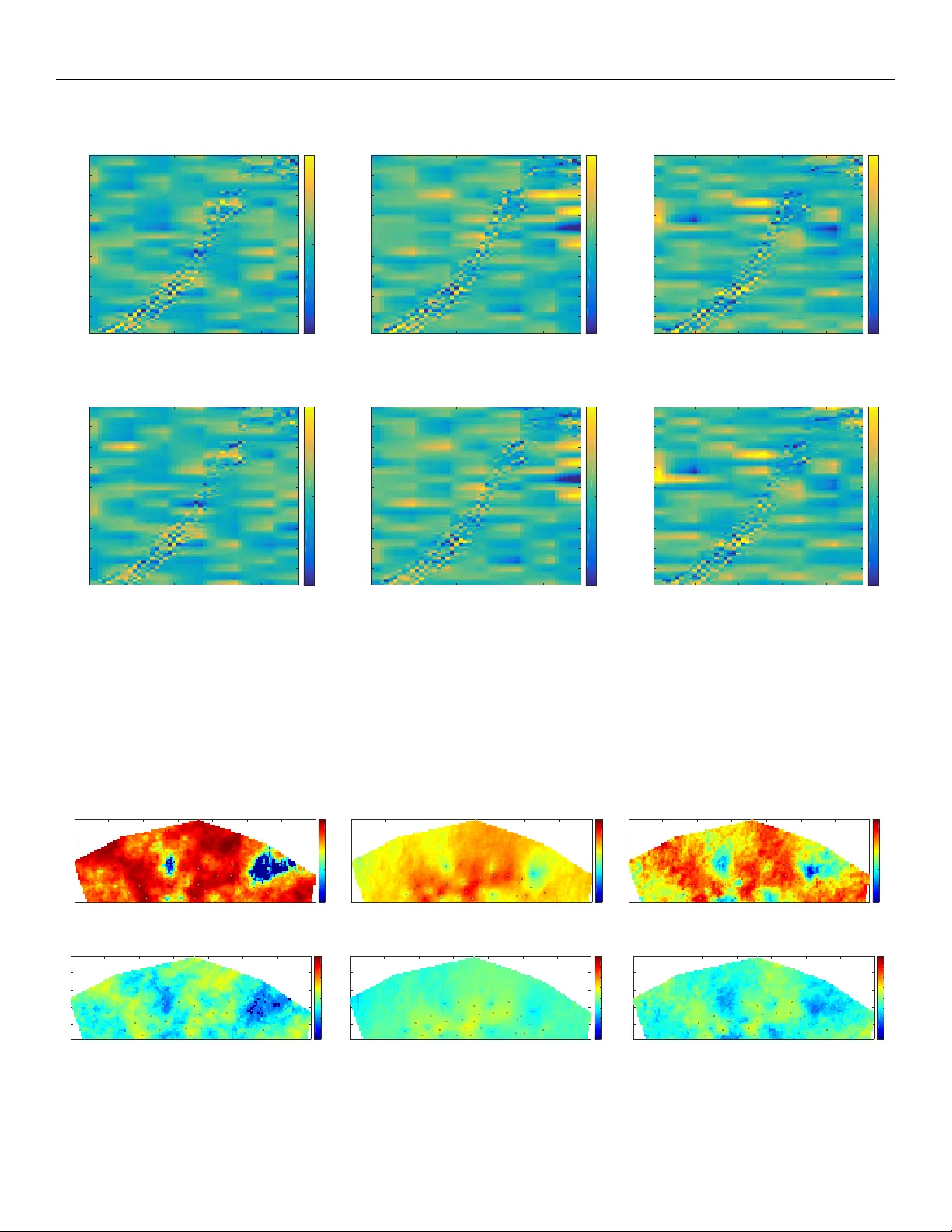
Efficient big data assimilation thr ough sparse representation: A 3D benchmark case study in seismic history matching Xiaodong Luo , SPE, IRIS; T uhin Bhakta, IRIS; Mor ten Jak obsen, UoB & IRIS; and Geir Nævdal, IRIS . Abstract In a previous work (Luo et al., 2016), the authors proposed an ensemble-based 4D seismic history matching (SHM) framework, which has some relati vely new ingredients, in terms of the type of seismic data in choice, the way to handle big seismic data and related data noise estimation, and the use of a recently dev eloped iterati v e ensemble history matching algorithm. In seismic history matching, it is customary to use in verted seismic attributes, such as acoustic impedance, as the observed data. In doing so, extra uncertainties may arise during the in v ersion processes. The proposed SHM framew ork av oids such intermediate in version processes by adopting amplitude versus angle (A V A) data. In addition, SHM typically inv olves assimilating a large amount of observed seismic attrib utes into reserv oir models. T o handle the big-data problem in SHM, the proposed framew ork adopts the following wa velet- based sparse representation procedure: First, a discrete wav elet transform is applied to observed seismic attributes. Then, uncertainty analysis is conducted in the wav elet domain to estimate noise in the resulting wav elet coefficients, and to calculate a corresponding threshold value. W av elet coef ficients above the threshold value, called leading wa velet coefficients hereafter , are used as the data for history matching. The retained leading wav elet coef ficients preserve the most salient features of the observ ed seismic attrib utes, whereas rendering a substantially smaller data size. Finally , an iterativ e ensemble smoother is adopted to update reservoir models, in such a way that the leading wa velet coef ficients of simulated seismic attributes better match those of observed seismic attrib utes. As a proof-of-concept study , Luo et al. (2016) applied the proposed SHM framework to a 2D case study , and numerical results therein indicated that the proposed framework worked well. Ho wever , the seismic attributes used in Luo et al. (2016) are 2D datasets with relativ ely small data sizes, in comparison to those in practice. In the current study , we extend our in vestigation to a 3D benchmark case, the Brugge field. The seismic attributes used are 3D datasets, with the total number of seismic data in the order of O (10 6 ) . Our study indicates that, in this 3D case study , the wa velet-based sparse representation is still highly efficient in substantially reducing the size of seismic data, whereas preserving the information content therein as much as possible. Meanwhile, the proposed SHM frame work also achieves reasonably good history matching performance. This in vestigation thus serves as an important preliminary step to wards applying the proposed SHM framew ork to real field case studies. Introduction Seismic is one of the most important tools used for reserv oir exploration, monitoring, characterization and management in the petroleum industry . Compared to con ventional production data used in history matching, seismic data is less frequent in time, but much denser in space. Therefore, complementary to production data, seismic data provide valuable additional information for reservoir characterization. There are different types of seismic data that one can use in history matching. Figure 1 provides an outline of the relation of some types of seismic data to reservoir petro-physical parameters (e.g., permeability and porosity) in forw ard simulations. As indicated there, using petro-physical parameters as the inputs to reserv oir simulators, one generates fluid saturation and pressure fields. Through a petro- elastic model (PEM), one obtains acoustic and/or shear impedance (or equi valently , compressional and/or shear velocities (velocity) and formation density) based on fluid saturation and/or pressure, and porosity . Finally , amplitude versus angle (A V A) data are computed by plugging impedance (or velocities and density) into an A V A equation (e.g., Zoeppritz equation, see, for e xample, A vseth et al., 2010). T o reduce the computational cost in forward simulations, many seismic history matching (SHM) studies use in verted seismic at- tributes that are obtained through seismic in versions. Such in verted properties can be, for instance, acoustic impedance (see, for example, Emerick and Reynolds, 2012; Emerick et al., 2013; Fahimuddin et al., 2010; Skjervheim et al., 2007) or fluid saturation fronts (see, for example, Abadpour et al., 2013; Leeuwenburgh and Arts, 2014; T rani et al., 2012). One issue in using in verted seismic attributes as the observational data is that, the y may not provide uncertainty quantification for the observ ation errors, since in verted seismic attributes are often obtained using certain deterministic in version algorithms. T ypically the volume of seismic data is huge, therefore SHM often constitutes a “big data assimilation” problem. For ensemble- based history matching algorithms, a big data size may lead to certain numerical problems, e.g., ensemble collapse and high costs in computing and storing Kalman gain matrices (Aanonsen et al., 2009; Emerick and Re ynolds, 2012). In addition, many history matching algorithms are de veloped for under-determined in verse problems, whereas a big data size could make the in verse problem become ov er- determined instead. This may thus affect the performance of history matching algorithms, as demonstrated in our previous study (Luo 2 Figure 1: Some types of seismic data and their relation to reserv oir petro-physical parameters. et al., 2016). Figure 2: W orkflow of w avelet-based sparse representation. In Luo et al. (2016), we proposed an ensemble-based 4D SHM framework in conjunction with a wav elet-based sparse representation procedure. W e take A V A attrib utes as the seismic data to avoid the extra uncertainties arising from a seismic inv ersion process. T o address of the issue of big data, we adopt a wav elet-based sparse representation procedure. Figure 2 explains the idea behind wavelet- based sparse representation. Given a set of seismic data (which can be 2D or 3D), one first applies a multilev el discrete wav elet transform (D WT) to the data. D WT is adopted for the following two purposes: one is to reduce the size of seismic data by exploiting the sparse representation nature of wavelet basis functions, and the other is to exploit its capacity of noise estimation in the wav elet domain (Donoho and Johnstone, 1995). Based on the estimated standard deviation (STD) of the noise, one can construct the corresponding observation error cov ariance matrix that is needed in many (including ensemble-based) history matching algorithms. For a chosen family of wav elet basis functions, seismic data are represented by the corresponding wav elet coefficients. When dealing with 2D data, D WT is similar to singular v alue decomposition (SVD) applied to a matrix. In the latter case, the matrix is represented by the corresponding singular v alues in the space spanned by the products of associated left and right singular v ectors. Like wise, in the 2D case, one can also draw similarities between wavelet-based sparse representation and truncated singular value decomposition (TSVD). Indeed, in D WT , small w avelet coef ficients are typically dominated by noise, whereas large coefficients mainly carry signal information (Jansen, 2012). Therefore, as will be demonstrated later , it is possible for one to use only a small subset of leading wav elet coefficients to capture the main features of the signal, while significantly reducing the number of wav elet coefficients. W e remark that TSVD-based sparse representation is not a suitable choice in the context of history matching, since the associated basis functions (i.e., products of left and right singular vectors) are data-dependent, meaning that in general it is not meaningful to compare and match the singular v alues of observed and simulated data. W av elet-based sparse representation in volves suppressing noise components in the wa velet domain. T o this end, we first estimate the STD of the noise in w avelet coef ficients, and then compute a threshold v alue that depends on both the noise STD and data size. One can substantially reduce the data size by only keeping leading wav elet coefficients above the threshold, while setting those belo w the threshold v alue to zero. The leading w av elet coefficients are then tak en as the (transformed) seismic data, and are history-matched using a certain algorithm. In the experiments later , we will examine the impact of the threshold v alue on the history matching performance. A number of ensemble-based SHM frame works have been proposed in the literature. For instance, Abadpour et al. (2013); Fahimud- din et al. (2010); Katterbauer et al. (2015); Leeuwenburgh and Arts (2014); Skjervheim et al. (2007); T rani et al. (2012) adopt the en- semble Kalman filter (EnKF) or a combination of the EnKF and ensemble Kalman smoother (EnKS), whereas Emerick and Reynolds 3 (2012); Emerick et al. (2013); Luo et al. (2016) employ the ensemble smoother with multiple data assimilation (ES-MD A), and re gular- ized Lev enburg-Marquardt (RLM) based iterati ve ensemble smoother (RLM-MA C, see Luo et al., 2015), respecti vely . W e note that the history matching algorithm itself is independent of the wav elet-based sparse representation procedure. Therefore, one may combine the sparse representation procedure with a generic history matching algorithm, whether it is ensemble-based or not. This work is or ganized as follows. First, we will introduce three key components of the proposed workflow , which includes: (1) forward A V A simulation, (2) 3D DWT based sparse representation procedure, and (3) regularized Levenb urg-Marquardt based iterative ensemble smoother . Then, we will apply the proposed frame work to the 3D Brugge benchmark case, and in vestigate the performance of the proposed frame work in v arious situations. Finally , we draw conclusions based on the results of our in vestig ation and discuss possible future works. The proposed frame work Figure 3: The proposed 4D seismic history matching frame work. The proposed frame work consists of three key components (see Figure 3), namely , forward A V A simulation, sparse representation (in terms of leading wavelet coefficients) of both observed and simulated A V A data, and the history matching algorithm. It is expected that the proposed framew ork can be also extended to other types of seismic data, and more generally , geophysical data with spatial correlations. Forward A V A simulation As can be seen in Figure 1, the forward A V A simulation in volves several steps. First, pore pressure and fluid saturations are generated through reserv oir flo w simulation that takes petro-physical (e.g., permeability and porosity) and other parameters as the inputs. The generated pressure and saturation values are then used to calculate seismic parameters, such as P- and S-wa ve velocities and densities of reserv oir and overb urden formations, through a petro-elastic model (PEM). Finally , a certain A V A equation is adopted to compute the A V A attributes at dif ferent angles or offsets. Building a proper PEM is crucial to the success of SHM, whereas it is a challenging task at the same time. T o interpret the changes in seismic response over time, an in-depth understanding of rock and fluid properties is required (Jack, 2001). In this study , since our focus is on v alidating the performance of the proposed framew ork in a 3D problem, we assume that the PEM is perfect. Here, we use a soft sand model as the PEM (Mavko et al., 2009). The model assumes that, the cement is deposited away from the grain contacts. It further considers that, the initial framework of the uncemented sand rock is densely random pack of spherical grains with the porosity (denote by φ hereafter) around 36%, which is the maximum porosity v alue that the rock could ha ve before suspension. For con venience of discussion later, we denote this value as the critical porosity ( φ c ) (Nur et al., 1991, 1998). The dry bulk modulus ( K H M ) and shear modulus ( µ H M ) at critical porosity can then be computed using the Hertz-Mindlin model (Mindlin, 1949) below K H M = n s C 2 p (1 − φ c ) 2 µ 2 s 18 π 2 (1 − ν s ) 2 P ef f , (1) and µ H M = 5 − 4 ν s 5(2 − ν s ) n s 3 C 2 p (1 − φ c ) 2 µ 2 s 2 π 2 (1 − ν s ) 2 P ef f , (2) where µ s , ν s , P ef f are grain shear modulus, Poisson’ s ratio, and effecti ve stress, respectiv ely . The coordination number C p denotes the av erage number of contacts per sphere, and n is the degree of root. Here, C p and n are set to 9 and 3, respectiv ely . 4 T o find the effecti ve dry moduli for a porosity value less than φ c , the modified Lower Hashin-Shtrikman (MLHS) bound can be used (Mavko et al., 2009). The MLHS connects two end points in the elastic modulus-porosity plane. One end point, ( K H M , µ H M ), corresponds to critical porosity φ c . The other end point corresponds to zero porosity , taking the moduli of the solid phase, i.e. quartz mineral ( K s , µ s ). For a porosity v alue φ between zero and φ c , the lower bound for dry rock effecti ve bulk K d and shear moduli G d can be expressed as K d = " φ φ c K H M + 4 3 µ H M + 1 − φ φ c K s + 4 3 µ H M # − 1 − 4 3 µ H M (3) and G d = " φ φ c µ H M + µ H M 6 Z + 1 − φ φ c µ s + µ H M 6 Z # − 1 − µ H M 6 Z , (4) respectiv ely , where K s is solid/mineral bulk modulus and Z = (9 K H M + 8 µ H M ) / ( K H M + 2 µ H M ) . Further , the saturation effect is incorporated using the Gassmann model (Gassmann, 1951). The saturated bulk modulus K sat and shear modulus µ sat can be expressed as K sat = K d + (1 − K d K s ) 2 φ K f + 1 − φ K s − K d K 2 s , (5) and µ sat = µ d , (6) respectiv ely , where K f is the effecti ve fluid bulk modulus, and is estimated using the Reuss av erage (Reuss, 1929). For an oil-water mixture (as is the case in the Brugge field), K f is giv en by K f = ( S w K w + S o K o ) − 1 , (7) where K w , K o , S w and S o are b ulk modulus of water/brine, bulk modulus of oil, saturation of water/brine and saturation of oil, respectiv ely . Further , the saturated density (Mavko et al., 2009) can be written as (for the water -oil mixture) ρ sat = (1 − φ ) ρ m + φS w ρ w + φS o ρ o , (8) where ρ sat , ρ m , ρ w and ρ o are saturated density of rock, mineral density , water/brine density and oil density , respectiv ely . Using the abov e equations, we can obtain P- and S-wa ve velocities gi ven by (Mavko et al., 2009) V P = s K sat + 4 3 µ sat ρ sat , (9) and V S = r µ sat ρ sat , (10) where V P and V S represent P- and S-wa ve v elocities, respectively . After seismic parameters are generated by plugging reservoir parameters into the PEM, we can then simulate seismogram based on these seismic parameters. First, the Zoeppritz equation is used to calculate the reflection coefficient at an interface between two layers. For multi-layer cases, we need to calculate reflectivity series as a function of two-way tra vel time (see, for example, Buland and Omre, 2003; Mavk o et al., 2009). Here, travel time is computed from the P-wa ve velocity and vertical thickness of each grid block. W e then conv olve the reflectivity series with a Ricker wavelet of 45 Hz dominant frequency to obtain the desired seismic A V A data. In the experiments later, we generate A V A data at two different angles (i.e. 10 ◦ and 20 ◦ ). W e use these A V A attributes directly without con verting them further to other attrib utes like intercept and gradient. In doing so, we av oid introducing extra uncertainties in the course of attribute con version. Sparse r epresentation and noise estimation in wa velet domain Let m ref ∈ R m denote the reference reservoir model. In the current study , we consider 3D A V A attributes (near- and far-of fset traces) in the form of p 1 × p 2 × p 3 arrays (tensors), where p 1 , p 2 and p 3 represent the numbers of inline, cross-line and time slices in seismic surve ys, respectiv ely . Accordingly , let g : R m → R p 1 × p 2 × p 3 be the forward simulator of A V A attributes. The observed A V A attributes d o are supposed to be the forward simulation g ( m ref ) with respect to the reference model, plus certain additiv e observation errors  , that is, d o = g ( m ref ) +  . (11) 5 For ease of discussion below , suppose at the moment that all the tensors in Eq. (11), i.e., d o , g ( m ref ) and  , are reshaped into vectors with p 1 × p 2 × p 3 elements. Throughout this study , we assume that, for a given A V A attribute, the elements of  are independently and identically distributed (i.i.d) Gaussian white noise, with zero mean but unknown variance σ 2 , where σ will be estimated through wa velet multiresolution analysis belo w . More generally , one may also assume that  follows a Gaussian distrib ution with zero mean and cov ariance σ 2 R , where R is a known covariance matrix and σ 2 is a scalar to be estimated. In this case, one can whiten the additive noise by multiplying both sides of Eq. (11) by R − 1 / 2 . As shown in Figure 2, wav elet-based sparse representation in volves the follo wing steps: (I) Apply D WT to seismic data; (II) Estimate noise STD of wavelet coef ficients; and (III) Compute a threshold value that depends on both noise STD and data size, and do thresholding accordingly . Figure 4: A single le vel decomposition in 3D decimated discrete wav elet transform. W e adopt 3D DWT to handle A V A attrib utes in this study . An introduction to wav elet theory is omitted here, and interested readers are referred to, for example, Mallat (2008). Figure 4 illustrates a single lev el decomposition in 3D D WT . For con venience, we call these three dimensions of A V A attributes x , y and z , respectively . The input data is d o LLL j , which can be either the original observation d o (when j = 0 ) or the partial data recovered using the wa velet coefficients of the sub-band LLL j (when j > 0 ). Without loss of generality , let us assume j = 0 , such that Figure 4 corresponds to the first lev el 3D wa velet transform. In this case, the 3D transform is achiev ed by sequentially applying 1D DWT along x , y and z directions. In the 1D DWT along each direction, there are both low- (L) and high-pass (H) filters, and the transform results in one “L ” and one “H” sub-band of wav elet coefficients, respectively . The “H” sub-band corresponds to high frequency components in wa velet domain, while the “L ” sub-band to lo w frequenc y ones. As a result, after the first lev el of 3D D WT , there are 8 sub-bands in the wav elet domain, which are labelled as LLL 1 , LLH 1 , LH L 1 , LH H 1 , H LL 1 , H LH 1 , H H L 1 and H H H 1 , respecti vely . The sub-band LLL 1 ( H H H 1 ) results only from lo w-pass (high-pass) filters, while the others from mixtures of lo w- and high-pass ones. One can continue the 3D D WT to the next le vel by applying the transform to the data d o LLL 1 that corresponds to the sub-band LLL 1 . This leads to a set of new sub-bands of wa velet coef ficients (labelled as LLL 2 , LLH 2 , LH L 2 , LH H 2 , H LL 2 , H LH 2 , H H L 2 and H H H 2 , respectiv ely), and so on. Since H H H 1 corresponds to the high frequency (typically noise) components of the original data d o , it can be used to infer noise STD in the wavelet domain. Specifically , let W and T denote orthogonal wa velet transform and thresholding operators, respectiv ely; ˜ d o = W ( d o ) stands for the whole set of wav elet coef ficients corresponding to the original data d o , and ˜ d o H H H 1 for the wavelet coefficients in the sub-band H H H 1 . After DWT and thresholding, the ef fectiv e observation system becomes T ◦ W ( d o ) = T ◦  W ◦ g ( m ref ) + W (  )  . (12) As will be discussed belo w , for leading wa velet coef ficients (those abov e the threshold value), T is an identity operator such that it does not modify the values of leading wa velet coef ficients. The reason for us to require orthogonal W is as follows: If W is orthogonal, then the wav elet transform preserves the energy of Gaussian white noise (e.g., the Euclidean norm of the noise term  ). In addition, like the power spectral distribution of white noise in frequency domain, the noise energy in the wav elet domain is uniformly distributed among all w avelet coefficients (Jansen, 2012). This implies that, if one can estimate the noise STD σ of small w avelet coefficients (e.g., those in H H H 1 ), then this estimation can also be used to infer the noise STD of leading wa velet coefficients used in history matching. Similar to our previous study Luo et al. (2016), the noise STD σ is estimated using the median absolute deviation (MAD) estimator (Donoho 6 and Johnstone, 1995): σ = median(abs( ˜ d o H H H 1 )) 0 . 6745 , (13) where abs( • ) is an element-wise operator , and takes the absolute value of an input quantity . After estimating σ in an n -level wav elet decomposition, we apply hard thresholding and select leading wavelet coefficients on the element-by-element basis, in a way such that T ( ˜ d o i ) =  0 if ˜ d o i < λ , ˜ d o i otherwise , (14) where, without loss of generality , the scalar ˜ d o i ∈ ˜ d o represents an indi vidual wa velet coef ficient, and λ is a certain threshold v alue to be computed later . Eq. (14) means that, for leading wav elet coefficients abov e (or equal to) the threshold λ , their values are not changed, whereas for those below λ , they are set to zero. Note that in Luo et al. (2016), hard thresholding is not applied to the coarsest sub-band (i.e., the LL n / LLL n sub-band for an n -le vel 2D/3D DWT) in light of the fact that the wav elet coefficients in this sub-band correspond to low-frequency components, which are typically dominated by the signal. As a result, applying thresholding to this sub-band may lead to certain loss of signal information in history matching. Howe ver , for an A V A attribute in this study , we hav e observed that its corresponding LLL n sub-band may contain a large amount of wa velet coefficients (e.g., in the order of 10 4 ). T o have the flexibility of efficiently reducing the data size, we lift the restriction such that thresholding can also be applied to the sub-band LLL n . In Luo et al. (2016), the threshold value λ is computed using the univ ersal rule (Donoho and Johnstone, 1994) λ = p 2 ln(# d o ) σ , (15) with # d o being the number of elements in d o . In the current work, when using Eq. (15) to select the threshold value, it is found that the resulting number of leading wa velet coef ficients may still be very large. As a result, in the experiments later , we select the threshold value according to λ = c p 2 ln(# d o ) σ , (16) where c > 0 is a positi ve scalar , and the larger the v alue of c , the less the number of leading wa velet coefficients. Therefore, the scalar c can be used to control the total number of leading wa velet coef ficients. Combining Eqs. (12) – (16), the effecti ve observ ation system in history matching becomes ˜ d o = W ◦ g ( m ref ) + W (  ) , for ˜ d o ≥ λ , (17) where now ˜ d o is a vector containing all selected leading wav elet coefficients, and W (  ) the corresponding noise component in the wa velet domain, with zero mean and co variance C ˜ d o = σ 2 I (here I is the identity matrix with a suitable dimension). W e use an example to illustrate the performance of sparse representation and noise estimation in 3D DWT . In this e xample, we first generate a reference A V A far-of fset trace using the forw ard A V A simulator . The dimension of this trace is 139 × 48 × 251 , therefore the data size is 1 , 674 , 672 . Figure 5(a) plots slices of the A V A trace at X = 40 , 80 , 120 , and Z = 50 , 100 , 150 and 200 , respectiv ely . W e then add Gaussian white noise to obtain the noisy A V A trace, with the noise le vel being 30% . Here, noise lev el is defined as: Noise lev el = variance of noise variance of pure signal . (18) Figure 5(b) shows slides of the noisy A V A trace at the same locations as in Figure 5(a). W e apply a three-level 3D D WT to the noisy data using Daubechies wa velets with two vanishing moments (Mallat, 2008), and use hard thresholding combined with the uni versal rule (Eqs. (13) – (15)) to select leading wav elet coef ficients. After thresholding, the number of leading wav elet coefficients reduces to 33 , 123 , only 2% of the original data size. On the other hand, by applying Eq. (13), the estimated noise STD is 0 . 0105 , and it is very close to the true noise STD 0 . 0104 . By applying an in verse 3D D WT to leading w av elet coefficients, we obtain the reconstructed A V A trace (Figure 5(c) plots slices of this trace at the same places as Figures 5(a) and 5(b)). Comparing Figures 5(a) – 5(c), one can see that, using leading w av elet coefficients that amounts to only 2% of the original data size, the slices of reconstructed A V A trace well capture the main features in the corresponding slices of the reference A V A data. Figures 5(d) – 5(f) show wav elet coefficients in the sub-bands H H L 1 of the reference, noisy and reconstructed A V A traces, respec- tiv ely . From these figures, one can see that, after applying thresholding to wav elet coefficients of noisy data (Figure 5(e)), the modified coefficients (Figure 5(f)) preserve those with large amplitudes in the reference case (Figure 5(d)). In general, the modified coefficients appear similar to those of the reference case, whereas certain small coefficients of the reference case are suppressed due to thresholding. Finally , Figures 5(g) – 5(i) depict slices of reference and estimated noise, and their difference, respectiv ely , at the same places as in Figure 5(a). Here, reference noise is defined as noisy A V A data (Figure 5(b)) minus reference A V A data (Figure 5(a)), estimated noise as noisy A V A data minus reconstructed A V A data (Figure 5(c)), and noise difference as estimated noise minus reference noise. The estimated noise appears very similar to the reference noise, although there are also certain differences according to Figure 5(i). This might be largely due to the fact that some small wa velet coefficients of the reference data are smeared out after thresholding, as aforementioned. 7 (a) Reference A V A far-offset trace (b) Noisy A V A far-offset trace (c) Reconstructed A V A far-offset trace 0 0.5 1 1.5 2 2.5 × 10 5 -0.4 -0.3 -0.2 -0.1 0 0.1 0.2 0.3 0.4 (d) H H L 1 of reference trace 0 0.5 1 1.5 2 2.5 × 10 5 -0.4 -0.3 -0.2 -0.1 0 0.1 0.2 0.3 0.4 (e) H H L 1 of noisy trace 0 0.5 1 1.5 2 2.5 × 10 5 -0.4 -0.3 -0.2 -0.1 0 0.1 0.2 0.3 0.4 (f ) H H L 1 of reconstructed trace (g) Reference noise (h) Estimated noise (i) Noise difference Figure 5: Illustration of sparse representation of a 3D A V A far -offset trace using slices at X = 40 , 80 , 120 and at Z = 50 , 100 , 150 , 200 , respectiv ely . (a) Reference A V A trace; (b) Noisy A V A trace obtained by adding Gaussian white noise (noise lev el = 30%) to the reference data; (c) Reconstructed A V A trace obtained by first conducting a 3D D WT on the noisy data, then applying hard thresholding (using the univ ersal threshold value) to wav elet coefficients, and finally reconstructing the data using an in verse 3D DWT based on the modified wa velet coefficients; (d) W avelet sub-band H H L 1 corresponding to the reference A V A data; (e) W avelet sub-band H H L 1 corresponding to the noisy A V A data; (f) W av elet sub-band H H L 1 corresponding to the reconstructed A V A data; (g) Reference noise, defined as noisy A V A data minus reference A V A data; (g) Estimated noise, defined as noisy A V A data minus reconstructed A V A data; (i) Noise difference, defined as estimated noise minus reference noise. All 3D plots are created using the package Slic e omatic (version 1.1) fr om MA TLAB Centr al (File ID: #764). 8 The ensemble history matching algorithm W e adopt the RLM-MA C algorithm (Luo et al., 2015) in history matching. W ithout loss of generality , let d o denote p -dimensional observations in history matching, which stands for values in the ordinary data space (e.g., 3D A V A attributes by reshaping 3D arrays into vectors), or their sparse representations in the transform domain (e.g., leading wa velet coefficients in wav elet domain). The observations d o are contaminated by Gaussian noise with zero mean and cov ariance C d (denoted by d o ∼ N ( 0 , C d ) ). Also denote by g the forward simulator that generates simulated observations d ≡ g ( m ) gi ven an m -dimensional reservoir model m . In the RLM-MA C algorithm, let M i ≡ { m i j } N e j =1 be an ensemble of N e reservoir models obtained at the i th iteration step, based on which we can construct two square root matrices used in the RLM-MA C algorithm. One of the matrices is in the form of S i m = 1 √ N e − 1  m i 1 − ¯ m i , · · · , m i N e − ¯ m i  ; ¯ m i = 1 N e N e X j =1 m i j , (19) and is called model square r oot matrix , in the sense that C i m ≡ S i m  S i m  T equals the sample cov ariance matrix of the ensemble M i . The other , defined as S i d = 1 √ N e − 1  g ( m i 1 ) − g ( ¯ m i ) , · · · , g ( m i N e ) − g ( ¯ m i )  , (20) is called data squar e r oot matrix for a similar reason. The RLM-MAC algorithm updates M i to a new ensemble M i +1 ≡ { m i +1 j } N e j =1 by solving the following minimum-average-cost problem argmin { m i +1 j } N e j =1 1 N e N e X j =1 h  d o j − g  m i +1 j  T C − 1 d  d o j − g  m i +1 j  + γ i  m i +1 j − m i j  T  C i m  − 1  m i +1 j − m i j  i , where d o j ( j = 1 , 2 , · · · , N e ) are perturbed observ ations generated by drawing N e samples from the Gaussian distribution N ( d o , C d ) , and γ i a positiv e scalar that can be used to control the step size of an iteration step, and is automatically chosen using a procedure similar to back-tracking line search (Luo et al., 2015). Through linearization, the MAC problem is approximately solved through the following iteration: m i +1 j = m i j + S i m ( S i d ) T  S i d ( S i d ) T + γ i C d  − 1  d o j − g  m i j  , for j = 1 , 2 , · · · , N e . (21) The stopping criteria have substantial impact on the performance of an iterativ e in version algorithm (Engl et al., 2000). Luo et al. (2015) mainly used the following tw o stopping conditions for the purpose of run-time control: (C1) RLM-MA C stops if it reaches a maximum number of iteration steps; (C2) RLM-MA C stops if the relati ve change of a verage data mismatch o ver two consecuti ve iteration steps is less than a certain v alue. For all the e xperiments later , we set the maximum number of iterations to 20 , and the limit of the relativ e change to 0 . 01% . Let Ξ i ≡ 1 N e N e X j =1 h  d o j − g  m i j  T C − 1 d  d o j − g  m i j  i (22) be the av erage (normalized) data mismatch with respect to the ensemble M i . Follo wing Proposition 6.3 of Engl et al. (2000), a third stopping condition is introduced and implemented in Luo et al. (2016). Concretely , we also stop the iteration in Eq. (21) when Ξ i < 4 p (23) for the first time, where the factor 4 is a critical v alue below which the iteration process starts to transit from con vergence to di vergence (Engl et al., 2000, page 158). Numerical results in Luo et al. (2016) indicate that, in certain circumstances, equipping RLM-MA C with the extra stopping condition (23) may substantially improve its performance in history matching. Readers are referred to Luo et al. (2016) for more details. In the current study , howe ver , the impact of the stopping criterion (23) is not as substantial as that in Luo et al. (2016). Nev ertheless, we prefer to keep this stopping criterion as an extra safeguard procedure. Numerical results in the Brugge benchmark case W e demonstrate the performance of the proposed workflo w through a 3D Brugge benchmark case study . T able 1 summarizes the key information of the experimental settings. Readers are referred to Peters et al. (2010) for more information of the benchmark case study . 9 T able 1: Summary of experimental settings in the Brugge benchmark case study Mo del dimension 139 × 48 × 9 (60048 gridblocks), with 44550 out of 60048 being activ e cells P arameters to estimate PORO, PERMX, PERMY, PERMZ. T otal num b er is 4 × 44550 = 178200 Gridblo c k size Irregular. Average ∆ X ≈ 93 m , ∆ Y ≈ 91 m , and av erage ∆ Z ≈ 5 m Reserv oir sim ulator ECLIPSE 100 (control mo de LRA T) Num b er of wells 10 injectors and 20 pro ducers Pro duction p erio d 3647.5 da ys (with 20 rep ort times) Pro duction data Pro duction wells : BHP , OPR and WCT; Injection wells : BHP . T otal n um b er: 20 × 70 = 1400 Seismic surv ey time Base: day 1; Monitor (1st): day 991; Monitor (2nd): da y 2999 4D seismic data A V A data from near- and far- offsets at three survey times. T otal n um b er: ∼ 7.02 M D WT (seismic) Three-lev el decomposition using 3D Daub ec hies wa velets with t w o v anishing moments Thresholding Hard thresholding based on Eqs.(14) and (16) History matc hing metho d iES (RLM-MA C) with an ensemble of 103 reserv oir models The Brugge field model has 9 layers, and each layer consists of 139 × 48 gridblocks. The total number of gridblocks is 60048, whereas among them 44550 are acti ve. The data set of the original benchmark case study does not contain A V A attributes, therefore we generate synthetic seismic data in the following way: The benchmark case contains an initial ensemble of 104 members. W e randomly pick one of them as the reference model (which turned out to be the member “FN-SS-KP-1-92”), and use the rest 103 members as the initial ensemble in this study . The model variables to be estimated include porosity (POR O) and permeability (PERMX, PERMY , PERMZ) at all activ e gridblocks. Consequently , the total number of parameters in estimation is 178200 . There are 20 producers and 10 water injectors in the reference model, and they are controlled by the liquid rate (LRA T) target. The production period is 10 years, and in history matching we use production data at 20 report times. The production data consist of oil production rates (WOPR) and water cuts (WWCT) at 20 producers, and bottom hole pressures (WBHP) at all 30 wells. Therefore the total number of production data is 1400 . Gaussian white noise is added to production data of the reference model. For WOPR and WWCT data, their noise STD are taken as the maximum v alues between 10% of their magnitudes and 10 − 6 (the latter is used to pre vent the numerical issue of division by zero), whereas for WBHP data, the noise STD is 1 bar . In the experiments, there are three seismic surv eys taking place on day 1 (base), day 991 (1st monitor), and day 2999 (2nd monitor), respectiv ely . At each survey , we apply forward A V A simulation described in the previous section to the static (porosity) and dynamic (pressure and saturation) v ariables of the reference model, and generate A V A attrib utes at two different angles: 10 ◦ (near-of fset) and 20 ◦ (far -of fset). Each A V A attribute is a 3D ( 139 × 48 × 176 ) cube, and consists of around 1 . 17 × 10 6 elements. Therefore the total number of 4D seismic data is around 3 × 2 × 1 . 17 × 10 6 = 7 . 02 × × 10 6 . For con venience of discussion later , we label the dimensions of the 3D cubes by X , Y and Z , respecti vely , such that X = 1 , 2 , · · · , 139 , Y = 1 , 2 , · · · , 48 and Z = 1 , 2 , · · · , 176 . In history matching, we add Gaussian white noise to each reference A V A attribute, with the noise le vel being 30% . Here we do not assume the noise STD is known. Instead, we first apply three-level 3D D WT to each A V A cube using Daubechies wa velets with tw o v anishing moments, and then use Eq. (13) to estimate noise STD in the wa velet domain. In what follows, we consider three history matching scenarios that in volve: (S1) production data only; (S2) 4D seismic data only; and (S3) both production and 4D seismic data. Because of the huge volumes of A V A attributes, in scenarios (S2) and (S3), it is not con venient to directly use the 4D seismic data in the original data space. Therefore, to examine the impact of data size on the performance of SHM, in each scenario (S2 or S3), we consider tw o cases that ha ve different numbers of leading w avelet coefficients. This is achiev ed by letting the scalar c of Eq. (16) be 1 and 5 , respecti vely . Results of scenario S1 (using pr oduction data only) Figure 6 shows the boxplots of data mismatch as a function of iteration step. The av erage data mismatch of the initial ensemble (iteration 0) is around 5 . 65 × 10 9 . After 20 iteration steps, the av erage data mismatch is reduced to 5431 . 97 , lower than the threshold value 4 × 1400 = 5600 in (23) for the first time. In this particular case, the stopping step selected according to the criterion (23) coincides with the maximum number of iteration steps. Therefore, we take the ensemble at the 20th iteration step as the final estimation. In this synthetic study , the reference reserv oir model is known. As a result, we use root mean squared error (RMSE) in the sequel to measure the ` 2 -distance (up to a factor) between an estimated model and the reference one. More specifically , let v tr be the ` -dimensional reference property , and ˆ v an estimation, then the RMSE e v of ˆ v with respect to the reference v tr is defined by e v = k ˆ v − v tr k 2 √ ` , (24) where k • k 2 denotes the ` 2 norm. 10 Iteration number 0 5 10 15 20 Data mismatch 10 4 10 6 10 8 10 10 Figure 6: Boxplots of production data mismatch as a function of iteration step (scenario S1). The horizontal dashed line indicates the threshold value ( 4 × 1400 = 5600 ) for the stopping criterion (23). For visualization, the vertical axis is in the logarithmic scale. In each box plot, the horizontal line (in red) inside the box denotes the median; the top and bottom of the box represent the 75th and 25th percentiles, respectiv ely; the whiskers indicate the ranges beyond which the data are considered outliers, and the whiskers positions are determined using the default setting of MA TLAB © R2015b, while the outliers themselves are plotted indi vidually as plus signs (in red). Iteration number 0 5 10 15 20 RMSE (PERMX) 1 1.2 1.4 1.6 1.8 2 2.2 (a) RMSEs of log PERMX Iteration number 0 5 10 15 20 RMSE (PORO) 0.02 0.025 0.03 0.035 0.04 0.045 (b) RM SEs of PORO Figure 7: Boxplots of RMSEs of (a) log PERMX and (b) POR O as functions of iteration step (scenario S1). 11 For brevity , Figure 7 reports the boxplots of RMSEs in estimating PERMX (in the natural log scale) and POR O, at different iteration steps, whereas the results for PERMY and PERMZ are similar to that for PERMX. As can be seen in Figure 7, the average RMSEs of both log PERMX and POR O tend to reduce as the number of iteration steps increases. Figure 8 shows the profiles of WBHP , WOPR and WWCT of the initial (1st ro w) and final (2nd row) ensemble at the producer BR-P-5. It is evident that, through history matching, the final ensemble matches the production data better than the initial one, and this is consistent with the results in Figure 6. For illustration, Figure 9 presents the reference log PERMX and POR O at layer 2 (1st column), the mean of log PERMX and POR O at layer 2 from the initial ensemble (2nd column), and the mean of log PERMX and PORO at layer 2 from the final ensemble (3rd column). A comparison between the initial and final estimates of log PERMX and POR O indicates that the final estimates appear more similar to the reference fields, in consistence with results in Figure 7. Results of scenario S2 (using seismic data only) T o examine the impact of data size on the performance of SHM, we consider two cases with different threshold values chosen through Eq. (16). In the first case, we let c = 1 , such that Eq. (16) reduces to the univ ersal rule in choosing the threshold value (Donoho and Johnstone, 1994). Under this choice, the number of leading wavelet coefficients is 178332 , around 2 . 5% of the original A V A data size ( 7 . 04 × 10 6 ). In the second case, we increase the value of c to 5 , such that the number of leading wa velet coef ficients further reduces to 1665 , which is more than 4000 times reduction in comparison to the original data size. Figure 10 indicates the boxplots of seismic data mismatch as functions of iteration step. In either case, seismic data mismatch reduces fast at the first fe w iteration steps, and then changes slowly afterwards. The stopping criterion (C2), monitoring the relativ e change of average data mismatch, becomes effecti ve in both cases, such that the iteration stops at the 11 th step when c = 1 , and at the 19 th when c = 5 . Accordingly , the ensembles at iteration step 11 and 19 , respecti vely , are taken as the final estimates in these two cases. In addition, it appears that ensemble collapse takes place in both cases, although this phenomenon is some what mitigated in the case c = 5 , in comparison to the case c = 1 . The mitigation of ensemble collapse is ev en more evident when we further increase c to 8 , and accordingly , reduce the data size to 534 . By doing so, howe ver , the history matching performance is deteriorated (results not included here), largely due to the fact that such a significant reduction of data size leads to substantial loss of information content in the seismic data, a point to be elaborated soon. Figure 11 sho ws boxplots of RMSEs of log PERMX (1st column) and POR O (2nd column) as functions of iteration step. It is clear that the RMSEs of the final ensembles are lo wer than those of the initial ones, e ven at c = 5 , the case in which data size is reduced more than 4000 times. On the other hand, when c = 1 (top row), the RMSEs of both log PERMX and POR O in the final ensemble are lower than those at c = 5 (bottom row). This indicates that, better history matching performance is achiev ed at c = 1 , with more information content captured in the leading wa velet coef ficients. As aforementioned, each 3D A V A cube is in the dimension of 139 × 48 × 176 . For illustration, the top row of Figure 12 indicates the slices of far -offset A V A cubes at X = 80 , with respect to the base survey (1st column), the 1st monitor survey (2nd column) and the 2nd monitor survey (3rd column), respecti vely , whereas the middle and bottom rows show the corresponding slices reconstructed using the leading wav elet coefficients (while setting other coef ficients to zero) at c = 1 and c = 5 , respectiv ely . Compared to figures in the top row , it is clear that the reconstructed ones at c = 1 capture the main features of the observed slices, while removing the noise component. Therefore in this case, although the univ ersal rule (corresponding to c = 1 ) still leads to a relativ ely large data size, it achiev es a good trade-of f between data size reduction and feature preserv ation. In contrast, at c = 5 , the seismic data size is significantly reduced. Howe ver , the reconstructed slices in the bottom row only retain a small portion of the strips in the observed slices of the top row , meaning that the data size is reduced at the cost of losing substantial information content of the seismic data. Nev ertheless, even with such an information loss, using the leading wav elet coefficients at c = 5 still leads to significantly improved model estimation in comparison to the initial ensemble, and this will become more evident when both production and seismic data are used in scenario S3. For brevity , in what follows we only present the results with respect to the case c = 1 . In the top row of Figure 13, we show the slices (at X = 80) of dif ferences between two groups of reconstructed f ar-offset A V A cubes. One group corresponds to the reconstructed far -of fset A V A cubes at three surve y times, using the leading wavelet coefficients ( c = 1 ) of the observed far-of fset A V A cubes. The other group contains the reconstructed far-of fset A V A cubes at three survey times, using the corresponding leading wa velet coefficients ( c = 1 ) of the mean simulated seismic data of the initial ensemble. Therefore the slices of differences in the top row can be considered as a reflection of the initial seismic data mismatch in Figure 10(a). Here, we use the slices of differences for ease of visualization, as the reconstructed slices of the observed and the mean simulated A V A cubes look very similar . Similarly , in the bottom ro w , we sho w the slices of differences between the reconstructed far-of fset A V A cubes of the observed seismic data, and the reconstructed far-of fset A V A cubes of the mean simulated seismic data of the final ensemble. In this case, the slices of differences can be considered as a reflection of the final seismic data mismatch in Figure 10(a). Comparing the top and bottom rows at a given surve y time, one can observe certain distinctions, which, howe ver , are not very significant in general. This is in line with the results in Figure 10(a), where the initial and final seismic data mismatch remain in the same order, in contrast to the substantial reduction of production data mismatch in scenario S1 (Figure 6). Similar to Figure 9, Figure 14 depicts the reference log PERMX and POR O at layer 2 (1st column), the mean of initial log PERMX and POR O at layer 2 (2nd column), and the mean of final log PERMX and PORO at layer 2 (3rd column). Compared to the initial mean estimates, the final mean log PERMX and POR O show clear improvements, in terms of the similarities to the reference fields. In addition, an inspection on the 3rd columns of Figures 9 and 14 reveals that the final mean estimates in S2 capture the geological structures of the reference fields better, especially in areas where there is neither injection nor production well (well locations are represented by 12 Time (days) 0 1000 2000 3000 BHP (psi) 0 500 1000 1500 2000 2500 BR-P-5 ens ref. meas. (a) WBHP of the initial ensemble Time (days) 0 1000 2000 3000 Oil production rate (m 3 /d) 0 500 1000 1500 2000 BR-P-5 ens ref. meas. (b) WOPR of the initial ensemble Time (days) 0 1000 2000 3000 Water cut 0 0.2 0.4 0.6 0.8 1 BR-P-5 ens ref. meas. (c) WW CT of the initial ensemble Time (days) 0 1000 2000 3000 BHP (psi) 1500 1600 1700 1800 1900 2000 2100 BR-P-5 ens ref. meas. (d) WBH P of the final ensemble Time (days) 0 1000 2000 3000 Oil production rate (m 3 /d) 400 600 800 1000 1200 1400 1600 1800 2000 BR-P-5 ens ref. meas. (e) W OPR of the final ensemble Time (days) 0 1000 2000 3000 Water cut 0 0.2 0.4 0.6 0.8 1 BR-P-5 ens ref. meas. (f ) WWCT of the final ensemble Figure 8: Profiles of WBHP , WOPR and WWCT of the initial (1st ro w) and final (2nd row) ensembles at the producer BR-P-5 (scenario S1). The production data of the reference model are plotted as orange curves, the observed production data at 20 report times as red dots, and the simulated production data of initial and final ensembles as blue curves. 13 20 40 60 80 100 120 10 20 30 40 PERMX; Layer: 2; Reference -2 0 2 4 6 8 (a) Re refrence log PERMX 20 40 60 80 100 120 10 20 30 40 PERMX; Layer: 2; Mean -2 0 2 4 6 8 (b) Mean of initial log PERMX 20 40 60 80 100 120 10 20 30 40 PERMX; Layer: 2; Mean -2 0 2 4 6 8 (c) Mean of final log PERMX 20 40 60 80 100 120 10 20 30 40 PORO; Layer: 2; Reference 0 0.1 0.2 0.3 0.4 (d) Rerefrence POR O 20 40 60 80 100 120 10 20 30 40 PORO; Layer: 2; Mean 0 0.05 0.1 0.15 0.2 0.25 0.3 0.35 0.4 (e) Mean of initial PORO 20 40 60 80 100 120 10 20 30 40 PORO; Layer: 2; Mean 0 0.05 0.1 0.15 0.2 0.25 0.3 0.35 0.4 (f ) Mean of final PORO Figure 9: Log PERMX (top row) and PORO (bottom row) of the reference reservoir model (1st column) and the means of the initial (2nd column) and final (3rd column) ensembles at Layer 2 (scenario S1). The black dots in the figures represent the locations of injection and production wells (top view). 0 1 2 3 4 5 6 7 8 9 10 11 Iteration number 2 3 4 5 6 7 8 9 Data mismatch × 10 6 (a) Se ismic data mismatch ( c = 1) 0 1 2 3 4 5 6 7 8 9 10111213141516171819 Iteration number 0 5 10 15 Data mismatch × 10 5 (b) Sei smic data mismatch ( c = 5) Figure 10: Boxplots of seismic data mismatch as functions of iteration step (scenario S2). Case (a) corresponds to the results with c = 1 , for which choice the number of leading wav elet coefficients is 178332 , roughly 2 . 5% of the original data size; Case (b) to the results with c = 5 , for which choice the number of leading wa velet coef ficients is 1665 , more than 4000 times reduction in data size. 14 0 1 2 3 4 5 6 7 8 9 10 11 Iteration number 1 1.2 1.4 1.6 1.8 2 2.2 RMSE (PERMX) (a) RMSEs of log PERMX ( c = 1) 0 1 2 3 4 5 6 7 8 9 10 11 Iteration number 0.02 0.025 0.03 0.035 0.04 0.045 RMSE (PORO) (b) RMSEs of PORO ( c = 1) 0 1 2 3 4 5 6 7 8 9 10 11 12 13 14 15 16 17 18 19 Iteration number 1 1.2 1.4 1.6 1.8 2 2.2 RMSE (PERMX) (c) RMSEs of log PERMX ( c = 5) 0 1 2 3 4 5 6 7 8 9 10 11 12 13 14 15 16 17 18 19 Iteration number 0.02 0.025 0.03 0.035 0.04 0.045 RMSE (PORO) (d) RMSEs of PORO ( c = 5) Figure 11: Boxplots of RMSEs of log PERMX (1st column) and POR O (2nd column) as functions of iteration step, with c being 1 (top) and 5 (bottom), respectiv ely (scenario S2). 15 Inline No. 80 10 20 30 40 Trace no. 20 40 60 80 100 120 140 160 Time(s) -0.2 -0.15 -0.1 -0.05 0 0.05 0.1 0.15 0.2 (a) Observ ed slice (base) Inline No. 80 10 20 30 40 Trace no. 20 40 60 80 100 120 140 160 Time(s) -0.2 -0.15 -0.1 -0.05 0 0.05 0.1 0.15 0.2 (b) Observed slice (1st mornitor) Inline No. 80 10 20 30 40 Trace no. 20 40 60 80 100 120 140 160 Time(s) -0.2 -0.15 -0.1 -0.05 0 0.05 0.1 0.15 0.2 (c) Observ ed slice (2st mornitor) Inline No. 80 10 20 30 40 Trace no. 20 40 60 80 100 120 140 160 Time(s) -0.2 -0.15 -0.1 -0.05 0 0.05 0.1 0.15 0.2 (d) Reconstructed (base) with c = 1 Inline No. 80 10 20 30 40 Trace no. 20 40 60 80 100 120 140 160 Time(s) -0.2 -0.15 -0.1 -0.05 0 0.05 0.1 0.15 0.2 (e) Reconstructed (1st mornitor) with c = 1 Inline No. 80 10 20 30 40 Trace no. 20 40 60 80 100 120 140 160 Time(s) -0.2 -0.15 -0.1 -0.05 0 0.05 0.1 0.15 0.2 (f ) Reconstructed (2st mornitor) with c = 1 Inline No. 80 10 20 30 40 Trace no. 20 40 60 80 100 120 140 160 Time(s) -0.2 -0.15 -0.1 -0.05 0 0.05 0.1 0.15 0.2 (g) Reconstructed (base) with c = 5 Inline No. 80 10 20 30 40 Trace no. 20 40 60 80 100 120 140 160 Time(s) -0.2 -0.15 -0.1 -0.05 0 0.05 0.1 0.15 0.2 (h) Re constructed (1st mornitor) with c = 5 Inline No. 80 10 20 30 40 Trace no. 20 40 60 80 100 120 140 160 Time(s) -0.2 -0.15 -0.1 -0.05 0 0.05 0.1 0.15 0.2 (i) Reconstructed (2st mornitor) with c = 5 Figure 12: T op row: slices of the observed far-of fset A V A cubes at X = 80 , with respect to the base survey (1st column), the 1st monitor surve y (2nd column) and the 2nd monitor surv ey (3rd column), respectiv ely . Middle row: corresponding reconstructed slices at X = 80 using the leading wav elet coefficients at c = 1 (while all other wa velet coef ficients are set to zero). Bottom row: corresponding reconstructed slices at X = 80 using the leading wa velet coefficients at c = 5 (while all other w avelet coef ficients are set to zero). 16 Inline No. 80 10 20 30 40 Trace no. 20 40 60 80 100 120 140 160 Time(s) -0.05 0 0.05 (a) Slic e of initial differerence (base) Inline No. 80 10 20 30 40 Trace no. 20 40 60 80 100 120 140 160 Time(s) -0.05 0 0.05 (b) Sli ce of initial differerence (1st mornitor) Inline No. 80 10 20 30 40 Trace no. 20 40 60 80 100 120 140 160 Time(s) -0.05 0 0.05 (c) Sl ice of initial differerence (2st mornitor) Inline No. 80 10 20 30 40 Trace no. 20 40 60 80 100 120 140 160 Time(s) -0.05 0 0.05 (d) Slice of final differerence (base) Inline No. 80 10 20 30 40 Trace no. 20 40 60 80 100 120 140 160 Time(s) -0.05 0 0.05 (e) Slice of final differerence (1st mornitor) Inline No. 80 10 20 30 40 Trace no. 20 40 60 80 100 120 140 160 Time(s) -0.05 0 0.05 (f ) Slice of final differerence (2st mornitor) Figure 13: T op row: slices (at X = 80 ) of the differences between the reconstructed far-of fset A V A cubes using the leading wavelet coefficients ( c = 1 ) of the observed seismic data, and the reconstructed far-of fset A V A cubes using the corresponding leading wa velet coefficients ( c = 1 ) of the means of the simulated seismic data of the initial ensemble. From left to right, the three columns correspond to the differences at the base, the 1st monitor , and the 2nd monitor surve ys, respectively . Bottom row: as in the top row , except that it is for the differences between the reconstructed f ar-of fset A V A cubes of the observed seismic data, and the reconstructed far -offset A V A cubes of the mean simulated seismic data of the final ensemble. 20 40 60 80 100 120 10 20 30 40 PERMX; Layer: 2; Reference -2 0 2 4 6 8 (a) Re refrence log PERMX 20 40 60 80 100 120 10 20 30 40 PERMX; Layer: 2; Mean -2 0 2 4 6 8 (b) Mean of initial log PERMX 20 40 60 80 100 120 10 20 30 40 PERMX; Layer: 2; Mean -2 0 2 4 6 8 (c) Mean of final log PERMX 20 40 60 80 100 120 10 20 30 40 PORO; Layer: 2; Reference 0 0.1 0.2 0.3 0.4 (d) Rerefrence POR O 20 40 60 80 100 120 10 20 30 40 PORO; Layer: 2; Mean 0 0.05 0.1 0.15 0.2 0.25 0.3 0.35 0.4 (e) Mean of initial PORO 20 40 60 80 100 120 10 20 30 40 PORO; Layer: 2; Mean 0 0.05 0.1 0.15 0.2 0.25 0.3 0.35 0.4 (f ) Mean of final PORO Figure 14: As in Figure 9, b ut for scenario S2 with c = 1 . 17 black dots in Figures 9 and 14). Results of scenario S3 (using both pr oduction and seismic data) In scenario S3, production and seismic (in terms of leading wa velet coefficients) data are assimilated simultaneously . Figure 15 reports the boxplots of production (top) and seismic (bottom) data mismatch as functions of iteration step. Because of the simultaneous assimilation of production and seismic data, the way to use the seismic data (in terms of the value of c in Eq. (16)) will affect the history matching results. This becomes evident if one compares the first and second columns of Figure 15. Indeed, when c = 1 , because the relativ ely lar ge data size, it is clear that ensemble collapse takes place in Figures 15(a) and 15(c). Also, the iteration stops at step 14, due to the stopping criterion (C2). By increasing c to 5, the size of seismic data is reduced from 178332 to 1665, and ensemble collapse seems mitigated to some extent, especially for production data, while the final iteration step is 19, due to the stopping criterion (C2). On the other hand, by comparing Figures 6, 10 and 15, it is clear that, in S3, the presence of both production and seismic data mak es the reduction of data mismatch dif ferent from the case of using either production or seismic data only . For instance, in the presence of seismic data, the production data mismatch (see Figures 15(a) and 15(b)) tend to be higher than that in Figure 6. On the other hand, with the influence of production data, the occurrence of ensemble collapse seems to be postponed in Figures 15(c) and 15(d), in comparison to those in Figure 10. Figure 16 shows boxplots of RMSEs of log PERMX (1st column) and POR O (2nd column) as functions of iteration step. Again, the RMSEs of the final ensembles are lower than those of the initial ones, for either c = 1 or c = 5 . On the other hand, a comparison of Figures 7, 11 and 16 indicates that the RMSEs of log PERMX and POR O (and similarly , the RMSEs of log PERMY and log PERMZ) are the lowest when using both production and seismic data in history matching. Using c = 5 in scenario S3 (Figures 16(c) and 16(d)) leads to higher RMSEs than using c = 1 . Nevertheless, they are still better than the RMSEs in scenario S1, and close to (for POR O) or better than (for log PERMX) those in scenario S2 with c = 1 (see Figures 11(a) and 11(b)). This suggests that, in this particular case, reasonably good history matching performance can still be achie ved, e ven though the data size is reduced more than 4000 times (at c = 5 ) through the wa velet-based sparse representation procedure. Again, for brevity , in what follows we only report the results with respect to the case c = 1 . Figure 17 shows the production data profiles at the producer BR-P-5 in scenario S3 with c = 1 . Clearly , compared to the initial ensemble, the final one matches the observed production data (red dots) better . Nevertheless, a comparison of the bottom ro ws of Figures 8 and 17 indicates that, the ensemble spreads of simulated production data (blue curves) tend to be under-estimated, such that the reference production data (yellow curves) are outside the profiles of simulated production data at certain time instances. Similar to Figure 13, in Figure 18 we sho w the slices (at X = 80) of differences between the reconstructed far -offset A V A cubes of observed and mean simulated seismic data, at three survey times. Again, compared to the slices with respect to the initial ensemble (top), there are some visible distinctions in the slices with respect to the final ensemble (bottom). Howe ver , if one compares the bottom rows of Figures 13 and 18, it seems that these slices look very similar to each other . This is consistent with the results in Figures 10(a) and 15(c), where the final seismic data mismatch of S2 and S3 remains close. Finally , Figure 19 compares the reference, initial and final mean log PERMX and PORO fields at layer 2. Again, the final mean estimates improve over the initial mean fields, in terms of the closeness to the references. In addition, a comparison of the final estimated fields (the 3rd columns) of Figures 9, 14 and 19 shows that the final mean estimates in S3 best capture the geological structures of the reference fields (the same observ ation is also obtained at c = 5 ). This indicates the benefits of using both production and seismic data in history matching. Discussions and conclusions In this work, we apply an efficient, ensemble-based seismic history matching framework to the 3D Brugge field case. The seismic data used in this study are near- and f ar-of fset amplitude versus angle (A V A) attributes, with the data size more than 7 million. T o handle the big data, we introduce a wav elet-based sparse representation procedure to substantially reduce the data size, while capturing the main features of the seismic data as many as possible. Through numerical experiments, we demonstrate the efficac y of the proposed history matching framework with the sparse representation procedure, even in the case that the seismic data size is reduced more than 4000 times. The size of seismic data (in the form of leading wa velet coef ficients) can be con veniently controlled through a threshold value. A relatively large threshold value means more reduction in data size, which is desirable for the history matching algorithm, but at the cost of extra information loss. In contrast, a relativ ely small threshold value results in a larger number of leading wav elet coefficients, hence better preserv es the information content of observed data. In this case, howe ver , the history matching algorithm may become more vulnerable to certain practical issues like ensemble collapse. As a result, the best practice would need to achieve a trade-off between reduction of data size and preservation of data information. Another observation from the experiment results is that, in this particular case, a combined use of production and seismic data in history matching leads to better estimation results than the cases of using either production or seismic data only . Ensemble collapse is clearly visible when seismic data is used in history matching. This phenomenon can be mitigated to some extent by increasing the threshold value (hence reducing the seismic data size), but it cannot be completely av oided. A possible remedy to this problem is to also introduce localization (see, for example, Chen and Oliver, 2010; Emerick and Reynolds, 2011) to the iterati ve ensemble smoother . In the presence of the sparse presentation procedure, howe ver , seismic data are transformed into wav elet domain, and the concept of “physical distance” may not be valid any more. As a result, localization will need to be adapted to this change. W e will in vestigate this issue in our future study . 18 0 1 2 3 4 5 6 7 8 9 10 11 12 13 14 Iteration number 10 4 10 6 10 8 10 10 Data mismatch (a) Pro duction data mismatch ( c = 1) 0 1 2 3 4 5 6 7 8 9 10 11 12 13 14 15 16 17 18 19 Iteration number 10 4 10 6 10 8 10 10 Data mismatch (b) Pro duction data mismatch ( c = 5) 0 1 2 3 4 5 6 7 8 9 10 11 12 13 14 Iteration number 2 3 4 5 6 7 8 9 Data mismatch × 10 6 (c) Seimic data mismatch ( c = 1) Iteration number 0 1 2 3 4 5 6 7 8 9 10111213141516171819 Data mismatch × 10 5 2 4 6 8 10 12 14 (d) Seimic data mismatch ( c = 5) Figure 15: Boxplots of production (top) and seismic (bottom) data mismatch as functions of iteration step (scenario S3). 19 0 1 2 3 4 5 6 7 8 9 10 11 12 13 14 Iteration number 0.8 1 1.2 1.4 1.6 1.8 2 2.2 RMSE (PERMX) (a) RMSEs of log PERMX ( c = 1) 0 1 2 3 4 5 6 7 8 9 10 11 12 13 14 Iteration number 0.02 0.025 0.03 0.035 0.04 0.045 RMSE (PORO) (b) RMSEs of PORO ( c = 1) Iteration number 0 1 2 3 4 5 6 7 8 9 10 11 12 13 14 15 16 17 18 19 RMSE (PERMX) 0.8 1 1.2 1.4 1.6 1.8 2 2.2 (c) RMSEs of log PERMX ( c = 5) Iteration number 0 1 2 3 4 5 6 7 8 9 10 11 12 13 14 15 16 17 18 19 RMSE (PORO) 0.02 0.025 0.03 0.035 0.04 0.045 (d) RMSEs of PORO ( c = 5) Figure 16: Boxplots of RMSEs of log PERMX (1st column) and POR O (2nd column) as functions of iteration step, with c being 1 (top) and 5 (bottom), respectiv ely (scenario S3). 20 Time (days) 0 1000 2000 3000 BHP (psi) 0 500 1000 1500 2000 2500 BR-P-5 ens ref. meas. (a) WBHP of the initial ensemble Time (days) 0 1000 2000 3000 Oil production rate (m 3 /d) 0 500 1000 1500 2000 BR-P-5 ens ref. meas. (b) WOPR of the initial ensemble Time (days) 0 1000 2000 3000 Water cut 0 0.2 0.4 0.6 0.8 1 BR-P-5 ens ref. meas. (c) WW CT of the initial ensemble 0 1000 2000 3000 Time (days) 1500 1600 1700 1800 1900 2000 2100 BHP (psi) BR-P-5 ens ref. meas. (d) WBH P of the final ensemble 0 1000 2000 3000 Time (days) 400 600 800 1000 1200 1400 1600 1800 2000 Oil production rate (m 3 /d) BR-P-5 ens ref. meas. (e) W OPR of the final ensemble 0 1000 2000 3000 Time (days) 0 0.2 0.4 0.6 0.8 1 Water cut BR-P-5 ens ref. meas. (f ) WWCT of the final ensemble Figure 17: As in Figure 8, b ut for the production data profiles in scenario S3 with c = 1 . 21 Inline No. 80 10 20 30 40 Trace no. 20 40 60 80 100 120 140 160 Time(s) -0.05 0 0.05 (a) Slic e of initial differerence (base) Inline No. 80 10 20 30 40 Trace no. 20 40 60 80 100 120 140 160 Time(s) -0.05 0 0.05 (b) Sli ce of initial differerence (1st mornitor) Inline No. 80 10 20 30 40 Trace no. 20 40 60 80 100 120 140 160 Time(s) -0.05 0 0.05 (c) Sl ice of initial differerence (2st mornitor) Inline No. 80 10 20 30 40 Trace no. 20 40 60 80 100 120 140 160 Time(s) -0.05 0 0.05 (d) Slice of final differerence (base) Inline No. 80 10 20 30 40 Trace no. 20 40 60 80 100 120 140 160 Time(s) -0.05 0 0.05 (e) Slice of final differerence (1st mornitor) Inline No. 80 10 20 30 40 Trace no. 20 40 60 80 100 120 140 160 Time(s) -0.05 0 0.05 (f ) Slice of final differerence (2st mornitor) Figure 18: As in Figure 18, b ut for the slices (at X = 80 ) of differences in scenario S3 with c = 1 . 20 40 60 80 100 120 10 20 30 40 PERMX; Layer: 2; Reference -2 0 2 4 6 8 (a) Re refrence log PERMX 20 40 60 80 100 120 10 20 30 40 PERMX; Layer: 2; Mean -2 0 2 4 6 8 (b) Mean of initial log PERMX 20 40 60 80 100 120 10 20 30 40 PERMX; Layer: 2; Mean -2 0 2 4 6 8 (c) Mean of final log PERMX 20 40 60 80 100 120 10 20 30 40 PORO; Layer: 2; Reference 0 0.1 0.2 0.3 0.4 (d) Rerefrence POR O 20 40 60 80 100 120 10 20 30 40 PORO; Layer: 2; Mean 0 0.05 0.1 0.15 0.2 0.25 0.3 0.35 0.4 (e) Mean of initial PORO 20 40 60 80 100 120 10 20 30 40 PORO; Layer: 2; Mean 0 0.05 0.1 0.15 0.2 0.25 0.3 0.35 0.4 (f ) Mean of final PORO Figure 19: As in Figure 9, b ut for scenario S3 with c = 1 . 22 Ackno wledgments W e would like to thank Schlumberger for providing us academic software licenses to ECLIPSE © . XL acknowledges partial financial supports from the CIPR/IRIS cooperativ e research project “4D Seismic History Matching” which is funded by industry partners Eni, Petrobras, and T otal, as well as the Research Council of Norway (PETROMAKS). All authors acknowledge the Research Council of Norway and the industry partners – ConocoPhillips Skandinavia AS, BP Nor ge AS, Det Norske Oljeselskap AS, Eni Nor ge AS, Maersk Oil Norway AS, DONG Energy A/S, Denmark, Statoil Petroleum AS, ENGIE E&P NORGE AS, Lundin Norway AS, Halliburton AS, Schlumberger Nor ge AS, Wintershall Nor ge AS – of The National IOR Centre of Norway for financial supports. References Aanonsen, S., Nævdal, G., Oliv er, D., Reynolds, A. and V all ` es, B. [2009] The Ensemble Kalman Filter in Reservoir Engineering: a Revie w . SPE Journal , 14 , 393–412. SPE-117274-P A. Abadpour , A., Bergey , P . and Piasecki, R. [2013] 4D Seismic History Matching With Ensemble Kalman Filter-Assimilation on Hausdorff Distance to Saturation Front. In: SPE Reservoir Simulation Symposium . Society of Petroleum Engineers. SPE-163635- MS. A vseth, P ., Mukerji, T . and Mavko, G. [2010] Quantitative seismic interpretation: Applying r ock physics tools to r educe interpretation risk . Cambridge University Press. Buland, A. and Omre, H. [2003] Bayesian linearized A VO in version. Geophysics , 68 , 185–198. Chen, Y . and Oliver , D.S. [2010] Cross-cov ariances and localization for EnKF in multiphase flow data assimilation. Computational Geosciences , 14 , 579–601. Donoho, D.L. and Johnstone, I.M. [1995] Adapting to unkno wn smoothness via wa velet shrinkage. J ournal of the American Statis- tical Association , 90 , 1200–1224. Donoho, D.L. and Johnstone, J.M. [1994] Ideal spatial adaptation by wa velet shrinkage. Biometrika , 81 , 425–455. Emerick, A. and Reynolds, A. [2011] Combining sensiti vities and prior information for cov ariance localization in the ensemble Kalman filter for petroleum reservoir applications. Computational Geosciences , 15 , 251–269. Emerick, A.A. and Reynolds, A.C. [2012] History matching time-lapse seismic data using the ensemble Kalman filter with multiple data assimilations. Computational Geosciences , 16 , 639–659. Emerick, A.A., Reynolds, A.C. et al. [2013] History-matching production and seismic data in a real field case using the ensemble smoother with multiple data assimilation. In: SPE Reservoir Simulation Symposium . Society of Petroleum Engineers. SPE-163675- MS. Engl, H.W ., Hanke, M. and Neubauer , A. [2000] Re gularization of Inver se Problems . Springer . Fahimuddin, A., Aanonsen, S. and Skjervheim, J.A. [2010] Ensemble Based 4D Seismic History Matching–Integration of Different Lev els and T ypes of Seismic Data. In: 72nd EA GE Conference & Exhibition . Gassmann, F . [1951] ¨ Uber die Elastizit ¨ at por ¨ oser Medien. V ierteljahr esschrift der Naturforschenden Gesellschaft , 96 , 1–23. Jack, I. [2001] The coming of age for 4D seismic. Fir st Break , 19 , 24–28. Jansen, M. [2012] Noise r eduction by wavelet thresholding , 161. Springer Science & Business Media. Katterbauer , K., Hoteit, I. and Sun, S. [2015] History matching of electromagnetically heated reservoirs incorporating full-wav efield seismic and electromagnetic imaging. SPE Journal , 20 , 923 – 941. SPE-173896-P A. Leeuwenbur gh, O. and Arts, R. [2014] Distance parameterization for efficient seismic history matching with the ensemble Kalman Filter . Computational Geosciences , 18 , 535–548. Luo, X., Bhakta, T ., Jakobsen, M. and Nævdal, G. [2016] An ensemble 4D seismic history matching framew ork with sparse repre- sentation based on wa velet multiresolution analysis. SPE Journal , in press. Luo, X., Stordal, A., Lorentzen, R. and Nævdal, G. [2015] Iterativ e ensemble smoother as an approximate solution to a regularized minimum-av erage-cost problem: theory and applications. SPE Journal , 20 , 962–982. SPE-176023-P A. Mallat, S. [2008] A wavelet tour of signal pr ocessing . Academic press. 23 Mavk o, G., Mukerji, T . and Dvorkin, J. [2009] The r ock physics handbook: Tools for seismic analysis of por ous media . Cambridge Univ ersity Press. Mindlin, R.D. [1949] Compliance of elastic bodies in contact. Journal of Applied Mechanics , 16 , 259–268. Nur , A., Marion, D. and Y in, H. [1991] W ave velocities in sediments. In: Shear waves in marine sediments , Springer , 131–140. Nur , A., Mavko, G., Dvorkin, J. and Galmudi, D. [1998] Critical porosity: A key to relating physical properties to porosity in rocks. The Leading Edge , 17 (3), 357–362. Peters, L., Arts, R., Brouwer , G., Geel, C., Cullick, S., Lorentzen, R.J., Chen, Y ., Dunlop, N., V ossepoel, F .C., Xu, R. et al. [2010] Results of the Brugge benchmark study for flooding optimization and history matching. SPE Reservoir Evaluation & Engineering , 13 , 391–405. Reuss, A. [1929] Berechnung der Fließgrenze von Mischkristallen auf Grund der Plastizit ¨ atsbedingung f ¨ ur Einkristalle. ZAMM- Journal of Applied Mathematics and Mechanics/Zeitschrift f ¨ ur Angewandte Mathematik und Mechanik , 9 , 49–58. Skjervheim, J.A., Evensen, G., Aanonsen, S.I., Ruud, B.O. and Johansen, T .A. [2007] Incorporating 4D seismic data in reserv oir simulation models using ensemble Kalman filter . SPE Journal , 12 , 282 – 292. SPE-95789-P A. T rani, M., Arts, R. and Leeuwenburgh, O. [2012] Seismic history matching of fluid fronts using the ensemble Kalman filter . SPE Journal , 18 , 159–171. SPE-163043-P A.