MIMO Graph Filters for Convolutional Neural Networks

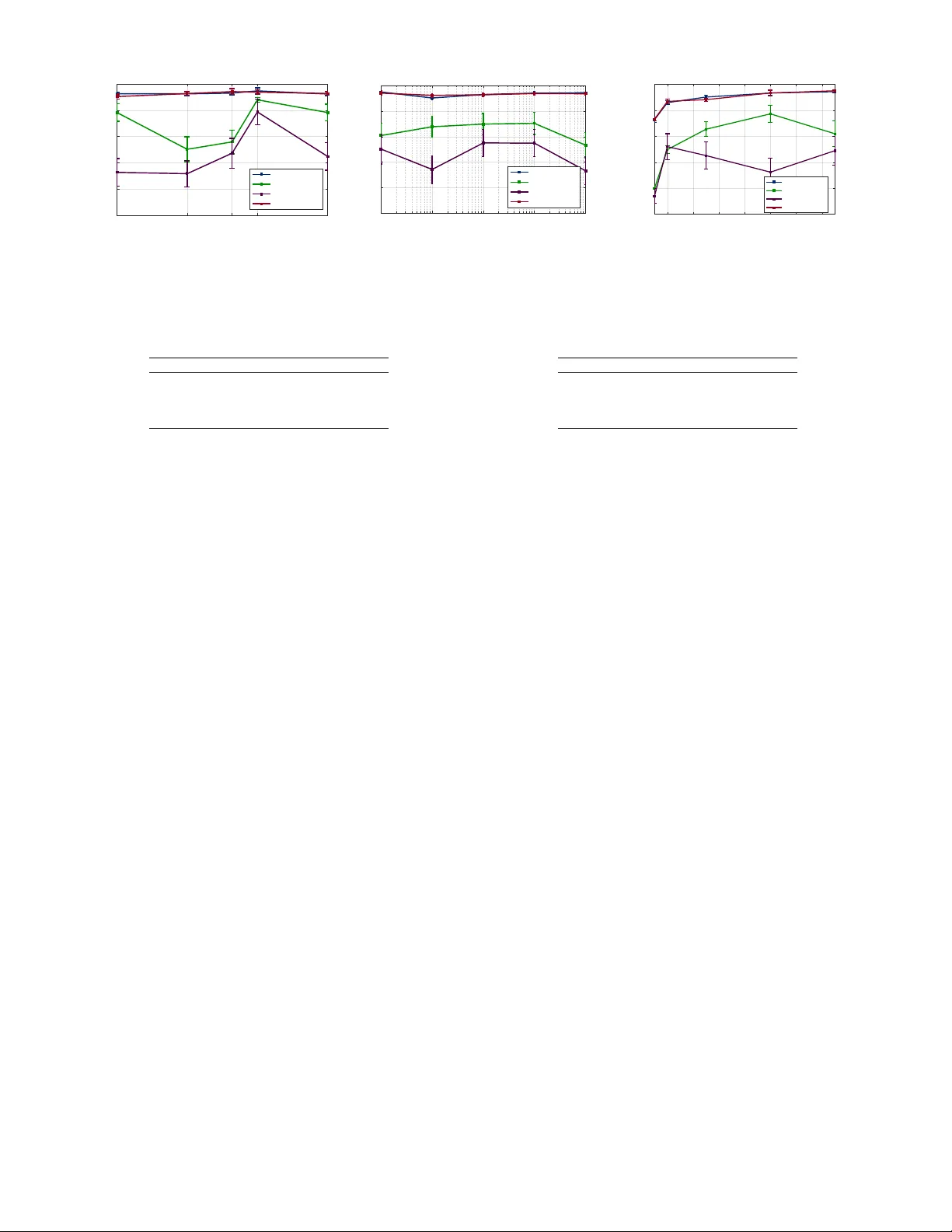
MIMO Graph Filters for Con v olutional Neural Networks Fer nando Gama, Antonio G. Marques, Alejandro Ribeiro, and Geert Leus Abstract —Superior performance and ease of implementation hav e foster ed the adoption of Con volutional Neural Networks (CNNs) f or a wide array of inference and reconstruction tasks. CNNs implement three basic blocks: con volution, pooling and pointwise nonlinearity . Since the two first operations are well- defined only on regular -structured data such as audio or im- ages, application of CNNs to contemporary datasets where the information is defined in irr egular domains is challenging. This paper in vestigates CNNs ar chitectures to operate on signals whose support can be modeled using a graph. Architectures that replace the regular con volution with a so-called linear shift-inv ariant graph filter ha ve been recently proposed. This paper goes one step further and, under the framework of multiple-input multiple- output (MIMO) graph filters, imposes additional structure on the adopted graph filters, to obtain three new (more parsimonious) architectur es. The pr oposed architectur es result in a lower num- ber of model parameters, reducing the computational complexity , facilitating the training, and mitigating the risk of ov erfitting. Simulations show that the proposed simpler architectur es achiev e similar perf ormance as mor e complex models. Index T erms —Con volutional neural networks, network data, graph signal processing, MIMO. I . I N T RO D U C T I O N Con volutional Neural Networks (CNNs) have emerged as the information processing architecture of choice in a wide range of fields as diverse as pattern recognition, computer vision and medicine, for solving problems in volving inference and reconstruction tasks [1]–[3]. CNNs have demonstrated remarkable performance, as well as ease of implementation and low online computational complexity [4], [5]. CNNs take the input data and process it through several layers, each of which performs three simple operations on the output of the previous layer . These three operations are con volution, pointwise nonlinearity and pooling. The objectiv e of such an architecture is to progressi vely extract useful information, from local features to more global aspects of the data. This is mainly achiev ed by the combination of con volution and pooling operations which sequentially combine data that is located further away . The nonlinearity dons the architecture with enough fle xibility to represent a richer class of functions that may describe the problem. One of the most outstanding characteristics of CNNs is that the filters used for con v olution can be efficiently learned from W ork supported by USA NSF CCF-1717120 and AR O W911NF1710438, Spanish MINECO grants No. TEC2013-41604-R and TEC2016-75361-R. F . Gama and A. Ribeiro are with the Dept. of Electrical and Systems Eng., Univ . of Pennsylvania., A. G. Marques is with the Dept. of Signal Theory and Comms., King Juan Carlos Uni v ., G. Leus is with the Dept. of Microelec- tronics, Delft Univ . of T echnology . Emails: { fgama,aribeiro } @seas.upenn.edu, antonio.garcia.marques@urjc.es, and g.j.t.leus@tudelft.nl . training datasets by means of a backpropagation algorithm [6]. This implies that the CNN architecture is capable of learning which are the most useful features for the task at hand. Intimately related to the capability of successful training, is the fact that the filters used are small, thus containing few parameters, making training easier . While, con volution and pooling are well-defined only in regular domains such as time or space, contemporary data is increasingly being described on domains that exhibit more irregular behavior [7], with examples including marketing, social networks, or genetics [8]–[10]. W ith the objectiv e of extending the remarkable performance of CNNs to broader data domains, extensions capable of processing netw ork data ha ve been de veloped [11]– [18], see [19] for a surv ey . In particular, the works of [11], [14] make use of the concept of graph filters (GFs) [20], [21] to extend the con v olution operation to graph signals [22]. Lev eraging the framework of multiple-input multiple-output (MIMO) GFs on existing results, this paper proposes three nov el architectures for GF-based CNNs. The main idea is to replace the bank of parallel GFs with a more structured filtering block which reduces the de grees of freedom (number of parameters) on each layer . This new architecture facilitates the training, incurs reduced computational complexity , and can be beneficial to av oid overfitting. Section II introduces notation and revie ws existing GF- based CNNs under the framework of MIMO GFs. Section III describes the novel architectures. Section IV presents simula- tions sho wing the benefits of our schemes. Concluding remarks are provided in Section V. I I . C N N S O N G R A P H S I G N A L S Let x ∈ X be the input data defined on some field X and let y ∈ Y be the output data such that y = f ( x ) for some (unknown) function f : X → Y . The general objective in machine learning is to estimate or learn the function f [23]. A neural network is an information processing architecture that aims at constructing an estimator ˆ f that consists of a concatenation of layers, each of which applies three simple operations on the output of the layer before, namely a linear transform, a pointwise nonlinearity and a pooling operator . Formally , the estimator ˆ f can be written as ˆ f = f L ◦ f L − 1 ◦ · · · ◦ f 1 where f ` denotes the operations to be applied at layer ` = 1 , . . . , L [24]. Denote by x ` ∈ X ` the N ` -dimensional output of layer ` defined over field X ` , by A ` : X ` − 1 → X 0 ` a linear transform between fields X ` − 1 and X 0 ` , by σ ` : X 0 ` → X 0 ` a pointwise nonlinearity , and by P ` : X 0 ` → X ` the pooling operator . Then, each layer can be described as x ` = f ` ( x ` − 1 ) = P ` { σ ` ( A ` x ` − 1 ) } , ` = 1 , . . . , L with X 0 ≡ X the input data field and X L ≡ Y the output data field. In particular , a CNN assumes that the linear operator A ` is comprised of a collection of F ` filters of small support K ` , A ` = { h `, 1 , . . . , h `,F ` } . Then, the application of the linear operator yields a collection of signals { h `, 1 ∗ x ` − 1 , . . . , h `,F ` ∗ x ` − 1 } , in which each element i = 1 , ..., N ` − 1 , [ h `,f ∗ x ` − 1 ] i = K ` − 1 X k =0 [ h `,f ] k [ x ` − 1 ] i − k (1) is considered a feature, f = 1 , . . . , F ` , and where we assumed that [ x ` − 1 ] i − k = 0 for i ≤ k . Using filters with a small support has a twofold goal. First, the con volution operation linearly relates nearby values (consecutiv e time instants, or neighboring pixels) and consolidates them in a feature v alue that aggregates this local information. Second, such filters only hav e a few parameters and, therefore, are easy to be learned from data. W e also note that the pooling operation serves the function of changing the r esolution of data, so that on each layer , the nearby v alues that are related by the conv olution operator are actually located further away . In this way , the con volution and pooling operations act in tandem to guarantee that the CNN aggre gates information at different lev els, from local to global. The operation of con volution, in particular , depends upon the existence of a notion of neighborhood. Such a notion also exists in domains like manifolds and graphs, and thus, the con volution can be extended to operate on signals defined on these irregular domains. In particular , for signals defined on graphs, let us start by considering the graph G = ( V , E , W ) , where V is the set of N nodes, E ⊆ V × V is the set of edges, and W : E → R is the function that assigns weights to the edges. The neighborhood of node i ∈ V is then defined as the set of nodes N i = { j ∈ V : ( j, i ) ∈ E } . With these notations in place, a graph signal is defined as a map which associates a real v alue to each element of V . This graph signal can be con veniently represented as the vector x ∈ R N , where the i -th element [ x ] i = x i corresponding to the v alue of the signal at node i . In order to relate the values of the graph signal at an y node with those at its neighborhood, we can mak e use of a matrix description of the graph. More precisely , let S ∈ R N × N be a gr aph shift operator (GSO) which is a matrix whose ( i, j ) -th element can be nonzero if and only if i = j or if ( j, i ) ∈ E [20]. Note then, that Sx is a linear combination of the values of the signal with that of its neighbors. More precisely , we ha ve that, for each i ∈ V [ Sx ] i = N X j =1 [ S ] ij x j = X j ∈N i ∪{ i } [ S ] ij x j (2) where the second equality follows because [ S ] ij = 0 if j / ∈ N i ∪ { i } . The operation in (2) is the basic element to extend the notion of con volution (filtering) to signals defined on graphs; see, e.g., [21]. First, observe that while Sx collects information from the one-hop neighborhood of each node, S k x collects information up to the k -hop neighborhood of each node. Denote by h = [ h 0 , . . . , h K − 1 ] T ∈ R K a collection of K filter taps. Then, we can linearly combine neighboring values up to the ( K − 1) -hop neighborhood by [cf. (1)] [ h ∗ x ] i = K − 1 X k =0 h k [ S k x ] i . (3) Upon defining matrix H := P K − 1 k =0 h k S k ∈ R N × N , (3) can be equiv alently written as h ∗ x = Hx = K − 1 X k =0 h k S k x . (4) with H being known as a linear shift-in v ariant (LSI) GF [21]. Since LSI-GFs are regarded as the generalization of con- volutions to operate on graph signals, the operator in (3) can be used to extend CNNs to operate on graph signals [11]. More specifically , assume that in each layer ` of the CNN, output x ` consists of F ` features, each of which is considered a graph signal x ( f ) ` ∈ R N ` × 1 defined on an N ` - node graph described by GSO S ` ∈ R N ` × N ` , f = 1 , . . . , F ` . Then, all F ` features can be concatenated on vector x ` = [( x (1) ` ) T , . . . , ( x ( F ` ) ` ) T ] T ∈ R F ` N ` × 1 . Assume that the linear transform A ` constructs F ` features out of the existing F ` − 1 ones. Then, A ` can be regarded as a MIMO GF since it takes F ` − 1 input signals and outputs F ` graph signals. By denoting as ⊗ the Kronecker matrix product, the output of the conv olution operation on graph signals can be compactly written as a MIMO GF as follows A ` x ` − 1 = K ` − 1 X k =0  H `,k ⊗ S k `  x ` − 1 (5) where H `,k ∈ R F ` × F ` − 1 contains the filter taps corresponding to the F ` − 1 F ` LSI-GFs employed. More precisely , by denoting as [ H `,k ] f ,f 0 = h ( ` ) k,f ,f 0 , the filter taps of the ( f , f 0 ) filter can be written as h ( ` ) f ,f 0 = [ h ( ` ) 0 ,f ,f 0 , . . . , h ( ` ) K ` − 1 ,f ,f 0 ] T ∈ R K ` × 1 , f = 1 , . . . , F ` , f 0 = 1 , . . . , F ` − 1 . Construction (5) builds F ` different LSI-GFs for each of the F ` − 1 features contained in the previous layer , totaling F ` − 1 F ` LSI-GFs. The total number of trainable parameters is thus F ` − 1 F ` K ` . While written differently , the MIMO GF in (5) represents the per- layer architecture proposed in [14]. Finally , with respect to the pooling operation, the use of multiscale hierarchical clustering to reduce the size of the graph in each layer has been employed, yielding N ` ≤ N ` − 1 and S ` the corresponding GSO of each layer [11], [14]. Also, due to the computational and performance issues of clustering, alternativ e approaches which do not rely on pooling exist [16]. In this work, we focus on the con volutional operation of CNNs on graph signals, letting the user determine the preferred choice of pooling scheme. I I I . C N N S B A S E D O N S T RU C T U R E D M I M O G F S This paper proposes three ne w architectures for CNNs on graph signals, obtained by imposing a certain parsimonious representation on the MIMO GF matrices { H `, 1 , . . . , H `,K ` } . The resulting architectures yield a considerably lower number of trainable parameters, reducing the complexity of the net- work, as well as av oiding certain pitfalls such as overfitting or the curse of dimensionality [25]. For simplicity , from now on, we focus on some specific layer ` , hence dropping the subscript on all notations. W e denote as x = x ` − 1 the input, with x = [ x T 1 , . . . , x T Q ] T ∈ R QN × 1 where x q ∈ R N are the F ` − 1 = Q input features, q = 1 , . . . , Q . W e denote as y = x ` the output features, with y = [ y T 1 , . . . , y T P ] T ∈ R P N × 1 where y p ∈ R N × 1 are the F ` = P output features, p = 1 , . . . , P . The length of the filters is K ` = K and the matrix of filter taps H `,k = H k ∈ R P × Q has elements [ H k ] p,q = h k,p,q , k = 0 , . . . , K − 1 , p = 1 , . . . , P , q = 1 , . . . , Q . Each of the ( p, q ) filters is represented by a vector of filter taps h p,q = [ h 0 ,p,q , . . . , h K − 1 ,p,q ] T ∈ R K × 1 . Equation (5) becomes y = K − 1 X k =0  H k ⊗ S k  x (6) and each new feature is computed as y p = Q X q =1 K − 1 X k =0 h k,p,q S k x q , p = 1 , . . . , P . (7) The design variables are the collection of matrices { H 0 , . . . , H K − 1 } containing the P Q filters, and thus totaling P QK parameters. A. Aggr egating the input features First, we propose to aggregate all input features so as to reduce the number of filters. Instead of designing P different filters for each one of the Q input features, we first aggregate the Q input features into one graph signal, and proceed to design P different filters to be applied to this graph signal. This strategy amounts to designing filter taps h p, 1 = [ h 0 ,p, 1 , . . . , h K − 1 ,p, 1 ] T ∈ R K × 1 for p = 1 , . . . , P . Then, matrix H k in (6) becomes a replication of the first column H k =      h k, 1 , 1 h k, 1 , 1 · · · h k, 1 , 1 h k, 2 , 1 h k, 2 , 1 · · · h k, 2 , 1 . . . . . . . . . . . . h k,P , 1 h k,P , 1 · · · h k,P , 1      . (8) Each output feature (7) is thus computed as y p = Q X q =1 K X k =1 h k,p, 1 S k x q = K X k =1 h k,p, 1 S k Q X q =1 x q ! (9) for p = 1 , . . . , P . Observe that the structure imposed on (8) leads to only P different LSI-GFs and therefore the number of trainable parameters has been reduced to P K . The effect of this filter , as observed from (9) is to first aggre gate all the input features into a single graph signal P Q q =1 x q and then applying P different filters to it, yielding the P different output features. B. Consolidating output features The second proposed architecture consists of designing one filter for each input feature and then consolidating all the filtered input features into a single output feature. In order to do this, we need to design Q LSI-GFs described by filter taps h 1 ,q = [ h 0 , 1 ,q , . . . , h K − 1 , 1 ,q ] T ∈ R K − 1 specific to each input feature q = 1 , . . . , Q . Matrix H k in (6) can thus be written as a replication of the first row H k =      h k, 1 , 1 h k, 1 , 2 · · · h k, 1 ,Q h k, 1 , 1 h k, 1 , 2 · · · h k, 1 ,Q . . . . . . . . . . . . h k, 1 , 1 h k, 1 , 2 · · · h k, 1 ,Q      . (10) This leads to each output feature (7) being calculated as y p = Q X q =1 K − 1 X k =0 h k, 1 ,q S k ! x q = Q X q =1 G q x q (11) for p = 1 , . . . , P . Note that all P output features y p are actually the same, since (11) does not depend on p . Thus, the filter taps gi ven by (10) actually yield a single output feature, which is the graph signal given by (11). This could be particularly useful for reducing operational complexity of subsequent layers, since graph signals can be handled easily . Observ e that the imposed structure (10) containing Q distinct filters yields QK trainable parameters. C. Convolution of features As a third approach to reducing the number of parameters in volv ed in (6), we consider a set of P + Q − 1 filters to be applied sequentially and progressiv ely to the input features, yielding output features that resemble conv olutions of the input features. Let h p − q +1 = [ h 0 ,p − q +1 , . . . , h K − 1 ,p − q +1 ] T ∈ R K − 1 be a set of filter taps, p = 1 , . . . , P , q = 1 , . . . , Q . Then, for this third proposed strategy , matrix H k in (6) becomes H k =      h k, 1 h k, 0 · · · h k, 2 − Q h k, 2 h k, 1 · · · h k, 3 − Q . . . . . . . . . . . . h k,P h k,P − 1 · · · h k,P +1 − Q      . (12) The output features are then obtained using (12) in (7) yielding y p = Q X q =1 K − 1 X k =0 h k,p +1 − q S k x q = K − 1 X k =0 S k Q X q =1 h k,p +1 − q x q (13) for p = 1 , . . . , P . From (13) we observe that each output feature y p can be thought of as the con volution of the input feature vector x with the collection of filter taps given by { h k,p , . . . , h k,p +1 − Q } . Note also that consecutive output features weigh input features similarly . In a way , (13) acts as a smoother of input features. Matrix H k in (12) is a T oeplitz matrix and thus has P + Q − 1 elements, so that the total number of trainable parameters is ( P + Q − 1) K . I V . N U M E R I C A L T E S T S Here we compare the performance of the three architectures proposed in Sections III-A, III-B and III-C, which in volve, respectiv ely , P K , QK and ( P + Q − 1) K parameters, with that of [14], which in volves P QK parameters [cf. (5)]. In the first testcase we consider a synthetic dataset of a source Probab ility of k eeping training sample 0.25 0.5 0.66 0.75 1 Accura cy 0 0.2 0.4 0.6 0.8 1 P K QK ( P + Q ! 1) K P QK (a) T est noise < 2 w 10 ! 5 10 ! 4 10 ! 3 10 ! 2 10 ! 1 Accura cy 0 0.2 0.4 0.6 0.8 1 P K QK ( P + Q ! 1) K P QK (b) Num b er of trainin g samples 2000 4000 6000 8000 10000 12000 14000 Accurac y 0 0.2 0.4 0.6 0.8 1 P K QK ( P + Q ! 1) K P QK (c) Figure 1: Accurac y in the source localization problem. Results were av eraged across 10 dif ferent graph realizations. For clarity of figures, error bars represent 1 / 4 of the estimated variance. (a) As a function of the probability of keeping a sample during the training phase, i.e. 1 − prob dropout . (b) As a function of the noise in the test set. (c) As a function of the number of training samples. Overall, we observ e that the full architecture (5) yields a performance similar to that proposed in Section III-A. Architecture Parameters Accuracy P QK 10 , 400 93 . 9% P K 480 94 . 8% QK 165 88 . 0% ( P + Q − 1) K 635 78 . 8% T able I: Source localization results for N = 16 nodes. localization problem in which different diffused graph signals are processed to determine the single node that originated them. In the second testcase we use the 20NEWS dataset and a word2vec embedding underlying graph to classify articles in one out of 20 different cate gories [26]. For both problems, we ev aluate an architecture with 2 conv olutional layers, the first one generating F 1 = 32 features, and the second one outputting F 2 = 64 features. GFs are of length K 1 = K 2 = K = 5 . No pooling is employed, so that N 1 = N 2 = N , the number of nodes in the graph, and S 1 = S 2 = S is the GSO specific to each testcase. W e denote as P QK the architecture in [14], and as P K , QK and ( P + Q − 1) K the ones developed in Sections III-A, III-B and III-C, respectiv ely . The number of parameters in the con volutional layers are 10400 for P QK , 480 for P K , 165 for QK and 635 for ( P + Q − 1) K . The selected nonlinearity is a ReLU applied at each layer and all architectures include a readout layer . For the training stage in both problems, an AD AM optimizer with learning rate 0 . 005 was employed [27], for 20 epochs and batch size of 100 . A. Source localization. Consider a connected Stochastic Block Model (SBM) graph with N = 16 nodes divided in 4 communities, with intra- community edge probability of 0 . 8 and intercommunity edge probability of 0 . 2 . Let W denote its adjacency matrix. W ith δ c representing a graph signal taking the v alue 1 at node c and 0 elsewhere, the signal x = W t δ c is a diffused version of the sparse input δ c for some unknown 0 ≤ t ≤ N − 1 . The objectiv e is to determine the source c that originated the signal x irrespecti ve of time t . T o that end, we create a set of N train labeled training samples { ( c 0 , x 0 ) } where x 0 = W t δ c 0 with both c 0 and t chosen at random. Then we create a test set with N test samples in the same fashion, but we add i.i.d. zero-mean Gaussian noise w with variance σ 2 w , so that the signals to be classified are W t δ c + w . The goal is to use the Architecture Parameters Accuracy P QK 10 , 400 61 . 32% P K 480 62 . 48% QK 165 58 . 22% ( P + Q − 1) K 635 64 . 06% T able II: Results for classification on 20NEWS dataset on a word2vec graph embedding of N = 5 , 000 nodes. training samples to design a CNN that determines the source (node) c that originated the diffused signal. First, we run the source localization problem on 10 dif ferent realizations of randomly generated SBM graphs. For each graph, we train the four architectures using dropout with probability of keeping each training sample of 0 . 75 . The total number of training samples is 10 , 000 . Once trained, the architectures are tested on a test set of 200 samples for each graph, contaminated with noise of variance σ 2 w = 10 − 1 . Results are listed in T able I, where the accuracy is av eraged ov er the 200 samples, over the 10 different graph realizations. W e observ e that the P K architecture proposed in Section III-A outperforms the full P QK architecture, with tw o orders of magnitude less parameters. Also, the QK and the ( P + Q − 1) K architectures yields reasonable performances. Additionally , we run tests changing the values of se veral of the simulations parameters. In Fig. 1a we observe the accuracy obtained when varying the probability of keeping training samples. It is noted that the P K architecture performs as well as the full P QK architecture. It is also observ ed that the other two architectures have significant variance, which implies that they depend hea vily on the topology of the graph. The ef fect of noise σ 2 w on the test samples can be observed in Fig. 1b. W e observe that all four architectures are relatively robust to noise. The QK and ( P + Q − 1) K architectures exhibit a dip in performance for the highest noise v alue simulated. Finally , in Fig. 1c we sho w the performance of all four architectures as a function of the number of training samples. W e see that the P K and the full P QK architecture improv e in performance as more training samples are considered, with a huge increase between 1 , 000 and 2 , 000 training samples. This same increase is observ ed for the remaining two architectures, although their performance behav es some what erratically afterwards. All in all, from these set of simulations, we observe that the P K architecture performs as well as the full P QK architecture, but utilizing almost two orders of magnitude less parameters. W e also observe that the QK and ( P + Q − 1) K architectures hav e a high dependence on the topology of the network. B. 20NEWS dataset Here we consider the classification of articles in the 20NEWS dataset which consists of 18 , 846 texts ( 11 , 314 of which are used for training and 7 , 532 for testing) [26]. The graph signals are constructed as in [14]: each document x is represented using a normalized bag-of-words model and the underlying graph support is constructed using a 16 -NN graph on the word2vec embedding [28] considering the 5 , 000 most common words. The GSO adopted is the normalized Laplacian. No dropout is used in the training phase. Accuracy results are listed in T able II, demonstrating that the P K and ( P + Q − 1) K architectures outperform the full P QK one, but requiring almost 100 times less parameters. V . C O N C L U S I O N S In this paper , we have studied the problem of extending CNNs to operate on graph signals. More precisely , we re- framed existing architectures under the concept of MIMO GFs, and lev eraged structured representations of such filters to reduce the number of trainable parameters inv olved. W e proposed three ne w architectures, each of which arises from adopting a different parsimonious model on the MIMO GF matrices. All the resulting architectures yield a lower number of trainable parameters, reducing computational complexity , as well as helping in av oiding certain pitfalls of training like ov erfitting or the curse of dimensionality . W e hav e applied the three proposed architectures to a synthetic problem on source localization, and compared its performance with the more complex, full MIMO GF model. W e analyzed performance as a function of dropout probability in the training phase, noise in the test samples, and number of training samples. W e noted that the proposed architecture that aggregates input features (Section III-A) has a performance similar to that of the full model, but inv olving two orders of magnitude less parameters. The other two architectures offer comparable performance for certain values of the analyzed parameters. Finally , we utilized the proposed architectures on the problem of classifying articles of the 20NEWS dataset. In this case, we observed that two of the proposed parsimonious models outperform the full model. R E F E R E N C E S [1] J. Bruna and S. Mallat, “In variant scattering conv olution networks, ” IEEE T rans. P attern Anal. Mach. Intell. , vol. 35, no. 8, pp. 1872–1886, Aug. 2013. [2] Y . LeCun, K. Kavukcuoglu, and C. Farabet, “Con volutional networks and applications in vision, ” in 2010 IEEE Int. Symp. Circuits and Syst. , Paris, France, 30 May-2 June 2010, IEEE. [3] H. Greenspan, B. v an Ginneken, and R. M. Summers, “Deep learning in medical imaging: Ov erview and future promise of an exciting new technique, ” IEEE Tr ans. Med. Imag. , vol. 35, no. 5, pp. 1153–1159, May 2016. [4] Y . LeCun, Y . Bengio, and G. Hinton, “Deep learning, ” Natur e , vol. 521, no. 7553, pp. 85–117, May 2015. [5] M. M. Najafabadi, F . V illanustre, T . M. Khoshgoftaar, and N. Seliya, “Deep learning applications and challenges in big data analytics, ” J. Big Data , vol. 2, no. 1, pp. 1–21, Dec. 2015. [6] D. E. Rumelhart, G. E. Hinton, and R. J. Williams, “Learning representations by back-propagating errors, ” Natur e , vol. 323, no. 6088, pp. 533–536, Oct. 1986. [7] D. Lazer et al., “Life in the network: The coming age of computational social science, ” Science , vol. 323, no. 5915, pp. 721–723, Feb . 2009. [8] M. O. Jackson, Social and Economic Networks , Princeton Uni versity Press, Princeton, NJ, 2008. [9] E. H. Davidson et al., “ A genomic regulatory network for dev elopment, ” Science , vol. 295, no. 5560, pp. 1669–1678, Feb . 2002. [10] J. Haupt, W . U. Bajwa, M. Rabbat, and R. Nowak, “Compressed sensing for networked data, ” IEEE Signal Pr ocess. Mag. , vol. 25, no. 2, pp. 92– 101, March 2008. [11] J. Bruna, W . Zaremba, A. Szlam, and Y . LeCun, “Spectral networks and deep locally connected networks on graphs, ” [cs.LG] , 21 May 2014. [12] M. Henaff, J. Bruna, and Y . LeCun, “Deep con volutional networks on graph-structured data, ” arXiv:1506.051631v1 [cs.LG] , 16 June 2015. [13] M. Niepert, M. Ahmed, and K. Kutzkov , “Learning con volutional neural networks for graphs, ” in 33rd Int. Conf . Mach. Learning , New Y ork, NY , 24-26 June 2016. [14] M. Defferrard, X. Bresson, and P . V andergheynst, “Con volutional neural networks on graphs with fast localized spectral filtering, ” in Neural Inform. Pr ocess. Syst. 2016 , Barcelona, Spain, 5-10 Dec. 2016, NIPS Foundation. [15] T . N. Kipf and M. W elling, “Semi-supervised classification with graph con volutional networks, ” in 5th Int. Conf. Learning Representations , T oulon, France, 24-26 Apr . 2017, Assoc. Comput. Linguistics. [16] F . Gama, G. J. T . Leus, A. G. Marques, and A. Ribeiro, “Con volutional neural networks via node-varying graph filters, ” [cs.LG] , 27 Oct. 2017. [17] B. Pasdeloup, V . Gripon, J.-C. V ialatte, and D. Pastor, “Con volutional neural netw orks on irre gular domains through approximate translations on inferred graphs, ” arXiv:1710.10035v1 [cs.DM] , 27 Oct. 2017. [18] J. Du, S. Zhang, G. W u, J. M. F . Moura, and S. Kar, “T opology adaptive graph con volutional networks, ” arXiv:1710.10370v2 [cs.LG] , 2 Nov . 2017. [19] M. M. Bronstein, J. Bruna, Y . LeCun, A. Szlam, and P . V andergheynst, “Geometric deep learning: Going beyond Euclidean data, ” IEEE Signal Pr ocess. Mag . , v ol. 34, no. 4, pp. 18–42, July 2017. [20] A. Sandyhaila and J. M. F . Moura, “Discrete signal processing on graphs: Frequenc y analysis, ” IEEE T rans. Signal Pr ocess. , vol. 62, no. 12, pp. 3042–3054, June 2014. [21] S. Segarra, A. G. Marques, and A. Ribeiro, “Optimal graph-filter design and applications to distributed linear network operators, ” IEEE Tr ans. Signal Process. , vol. 65, no. 15, pp. 4117–4131, Aug. 2017. [22] A. Sandryhaila and J. M. F . Moura, “Discrete signal processing on graphs, ” IEEE T rans. Signal Pr ocess. , vol. 61, no. 7, pp. 1644–1656, Apr . 2013. [23] M. J. Kearns and U. V . V azirani, An Intr oduction to Computational Learning Theory , The MIT Press, Cambridge, MA, 1994. [24] I. Goodfellow , Y . Bengio, and A. Courville, Deep Learning , The Adaptiv e Computation and Machine Learning Series. The MIT Press, Cambridge, MA, 2016. [25] G. Huang, Z. Liu, L. v an der Maaten, and K. Q. W einberger , “Densely connected con volutional networks, ” in IEEE Comput. Soc. Conf. Comput. V ision and P attern Recognition 2017 , Honolulu, HI, 21-26 July 2017, IEEE Comput. Soc. [26] T . Joachims, “ Analysis of the Rocchio algorithm with TFIDF for text categorization, ” Computer Science T echnical Report CMU-CS-96-118, Carnegie Mellon Uni versity , 1996. [27] D. P . Kingma and J. L. Ba, “AD AM: A method for stochastic optimization, ” in 3rd Int. Conf. Learning Representations , San Diego, CA, 7-9 May 2015, Assoc. Comput. Linguistics. [28] T . Mikolov , K. Chen, G. Corrado, and J. Dean, “Efficient estimation of word representations in vector space, ” in 1st Int. Conf. Learning Repre- sentations , Scottsdale, AZ, 2-4 May 2013, Assoc. Comput. Linguistics.