A theory of sequence indexing and working memory in recurrent neural networks

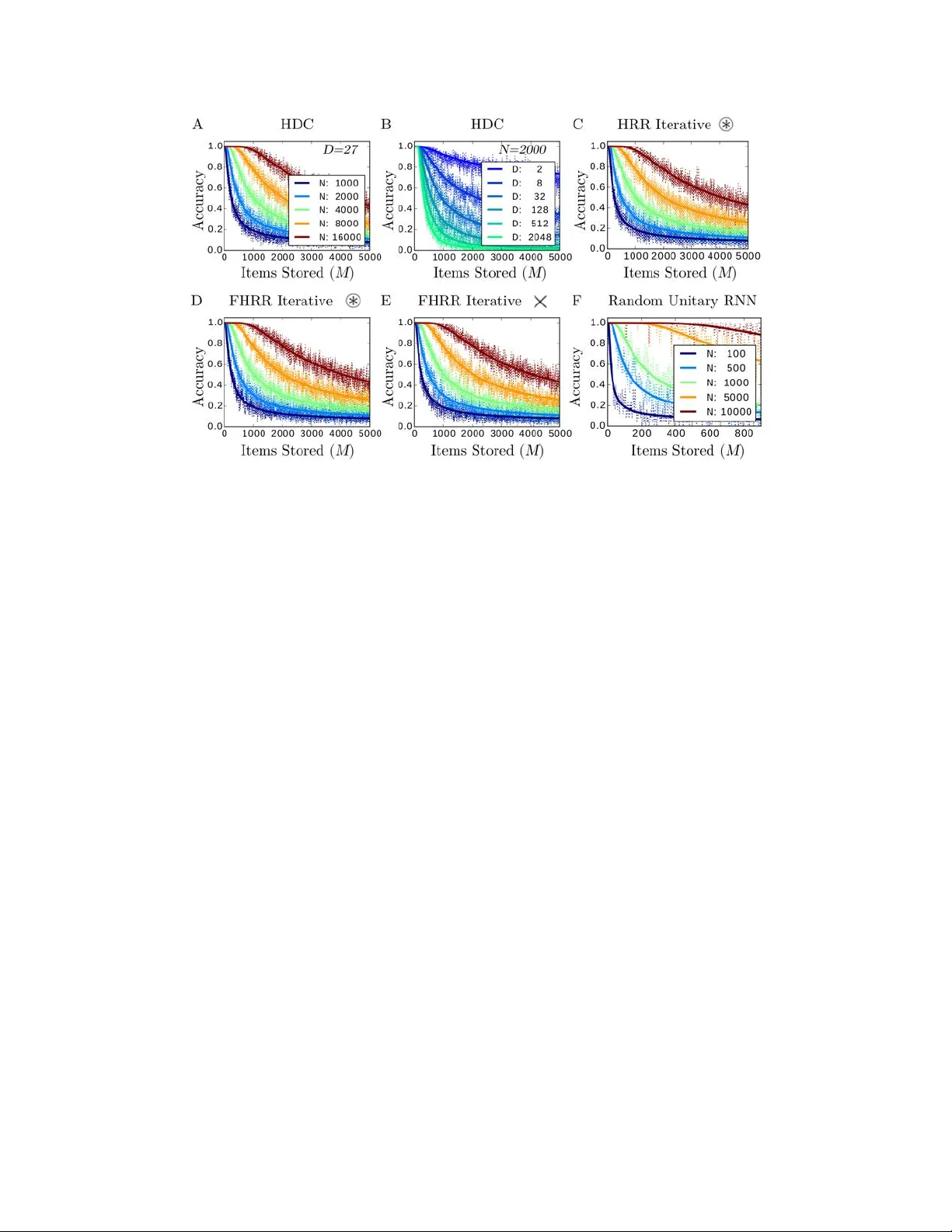
1 A theory of sequence indexing and working memory in r ecurr ent neural networks E. Paxon Frady 1 , Denis Kleyko 2 , Friedrich T . Sommer 1 1 Redwood Center for Theoretical Neuroscience, U.C. Berkele y 2 Department of Computer Science, Electrical and Space Engineering, Lulea Uni versity of T echnology K eywords: Recurrent neural networks, information theory , vector symbolic architec- tures, working memory , memory b uffer , reservoir computing Running Title: Inde xing and memory in neural networks Abstract T o accommodate structured approaches of neural computation, we propose a class of recurrent neural networks for inde xing and storing sequences of symbols or analog data vectors. These networks with randomized input weights and orthogonal recurrent weights implement coding principles previously described in vector symbolic ar chitec- tur es (VSA), and lev erage properties of r eservoir computing . In general, the storage in reservoir computing is lossy and crosstalk noise limits the retrie val accuracy and in- formation capacity . A nov el theory to optimize memory performance in such networks is presented and compared with simulation experiments. The theory describes linear readout of analog data, and readout with winner-take-all error correction of symbolic data as proposed in VSA models. W e ﬁnd that div erse VSA models from the literature hav e univ ersal performance properties, which are superior to what previous analyses predicted. Further , we propose nov el VSA models with the statistically optimal W iener ﬁlter in the readout that exhibit much higher information capacity , in particular for stor - ing analog data. The presented theory also applies to memory buf fers, networks with gradual forgetting, which can operate on inﬁnite data streams without memory ov erﬂo w . Interestingly , we ﬁnd that dif ferent for getting mechanisms, such as attenuating recurrent weights or neural nonlinearities, produce very similar beha vior if the forgetting time constants are aligned. Such models exhibit extensive capacity when their for getting time constant is optimized for giv en noise conditions and network size. These results enable the design of ne w types of VSA models for the online processing of data streams. 1 Intr oduction An important aspect of information processing is data representation. In order to ac- cess and process data, addresses or ke ys are required to provide a necessary context. T o enable ﬂe xible conte xtual structure as required in cogniti ve reasoning, connectionist models ha ve been proposed that represent data and keys in a high-dimensional v ector space. Such models include holographic reduced representations (HRR) (Plate, 1991, 2003), and hyperdimensional computing (HDC) (Gayler, 1998; Kanerva, 2009), and will be referred to here by the umbrella term vector symbolic ar chitectur es (VSA; see Gayler (2003); Methods 4.1.1). VSA models hav e been sho wn to be able to solv e chal- lenging tasks of cognitiv e reasoning (Rinkus, 2012; Kleyko and Osipov , 2014; Gayler, 2003). VSA principles have been recently incorporated into standard neural networks for challenging machine-learning tasks (Eliasmith et al., 2012), inducti ve reasoning (Rasmussen and Eliasmith, 2011), and processing of temporal structure (Gra ves et al., 2014, 2016; Danihelka et al., 2016). T ypically , VSA models offer at least two dif fer - ent kinds of operation, one to produce key-v alue bindings (also referred to as role-ﬁller pairs), and a superposition operation that forms a working memory state containing the index ed data structures. For e xample, to represent a time sequence of data in a VSA, indi vidual data points are bound to time-stamp keys and the resulting ke y-v alue pairs superposed into a working memory state. Here, we sho w that input sequences can be indexed and memorized according to vari- ous e xisting VSA models by recurrent neural networks (RNNs) that hav e randomized input weights and orthonormal recurrent weights of particular properties. Con versely , this class of netw orks has a straight-forw ard computational interpretation: in each cy- cle, a ne w random ke y is generated, a ke y-value pair is formed with the new input, and the index ed input is integrated into the network state. In the VSA literature, this operation has been referred to as tr ajectory association (Plate, 1993). The memory in these networks follo ws principles previously described in r eservoir computing . The idea of reservoir computing is that a neural netw ork with ﬁxed recurrent connecti vity can exhibit a rich reserv oir of dynamic internal states. An input sequence can selectiv ely e vok e these states so that an additional decoder network can extract the input history from the current network state. These models produce and retain neural representations of inputs on the ﬂy , entirely without relying on previous synaptic learning as in standard models of neural memory networks (Caianiello, 1961; Little and Shaw, 1978; Hopﬁeld, 1982; Schwenker et al., 1996; Sommer and Dayan, 1998). Models of reservoir comput- ing include state-dependent networks (Buonomano and Merzenich, 1995), echo-state networks (Jaeger, 2002; Luko ˇ se vi ˇ cius and Jaeger, 2009), liquid-state machines (Maass et al., 2002), and related netw ork models of memory (White et al., 2004; Ganguli et al., 2008; Sussillo and Abbott, 2009). Ho we ver , it is unclear how such reservoir models create representations that enables the selecti ve readout of past input items. Le veraging the structured approach of VSAs to compute with distrib uted representations, we of fer 2 a nov el frame work for understanding reserv oir computing. 2 Results 2.1 Indexing and memorizing sequences with r ecurrent netw orks Network model: W e in v estigate how a sequence of M input vectors of dimension D can be indexed by pseudo-random vectors and memorized by a recurrent network with N neurons (Fig. 1). The data vectors a ( m ) ∈ I R D are fed into the network through a randomized, ﬁxed input matrix Φ ∈ I R N × D . In the context of VSA, the input matrix corresponds to the codebook , the matrix columns contain the set of high-dimensional random vector - symbols ( hypervectors ) used in the distributed computation scheme. In addition, the neurons might also e xperience some independent neuronal noise η ( m ) ∈ I R N with p ( η i ( m )) ∼ N (0 , σ 2 η ) . Further , feedback is provided through a matrix of recurrent weights λ W ∈ I R N × N where W is orthogonal and 0 < λ ≤ 1 . The input sequence is encoded into a single network state x ( M ) ∈ I R N by the recurrent neural network (RNN): x ( m ) = f ( λ Wx ( m − 1) + Φa ( m ) + η ( m )) (1) with f ( x ) the component-wise neural activ ation function. T o estimate the input a ( M − K ) entered K steps ago from the network state, the readout is of the form: ˆ a ( M − K ) = g ( V ( K ) > x ( M )) (2) where V ( K ) ∈ I R N × D is a linear transform to select the input that occurred K time steps in the past (Fig. 1). In some models, the readout includes a nonlinearity g ( h ) to produce the ﬁnal output. Figure 1: Network model in vestigated. The ef fect of one iteration of equation (1) on the probability distribution of the net- work state x ( m ) is a Markov chain stochastic process, governed by the Chapman- 3 K olmogorov equation (P apoulis, 1984): p ( x ( m + 1) | a ( m )) = Z p ( x ( m + 1) | x ( m ) , a ( m )) p ( x ( m )) d x ( m ) (3) with a transition kernel p ( x ( m + 1) | x ( m ) , a ( m )) , which depends on all parameters and functions in (1). Thus, to analyze the memory performance in general, one has to iterate equation (3) to obtain the distribution of the netw ork state. Properties of the matrices in the encoding netw ork: The analysis simpliﬁes considerably if the input and recurrent matrix satisfy certain conditions. Speciﬁcally , we in vestig ate networks in which the input matrix Φ has i.i.d. random entries and the recurrent weight matrix W is orthogonal with mixing properties and long cycle length. The assumed properties of the network weights guarantee the follo wing independence conditions of the indexing ke ys, which will be essential in our analysis of the network performance: • Code v ectors Φ d are composed of identically distributed components: p (( Φ d ) i ) ∼ p Φ ( x ) ∀ i, d (4) where p Φ ( x ) is the distribution for a single component of a random code vector , and with E Φ ( x ) , V Φ ( x ) being the mean and v ariance of p Φ ( x ) , as typically de- ﬁned by E Φ ( φ ( x )) := R φ ( x ) p Φ ( x ) dx , V Φ ( φ ( x )) := E Φ ( φ ( x ) 2 ) − E Φ ( φ ( x )) 2 , with φ ( x ) an arbitrary function. • Components within a code v ector and between code vectors are independent : p (( Φ d 0 ) i , ( Φ d ) j ) = p (( Φ d 0 ) i ) p (( Φ d ) j ) ∀ j 6 = i ∨ d 0 6 = d (5) • The recurrent weight matrix W is orthogonal and thus pr eserves mean and vari- ance of e very component of a code v ector: E (( WΦ d ) i ) = E (( Φ d ) i ) ∀ i, d V ar (( WΦ d ) i ) = V ar (( Φ d ) i ) ∀ i, d (6) • The recurrent matrix preserves element-wise independence with a lar ge cycle time (around the size of the reservoir): p (( W m Φ d ) i , ( Φ d ) i ) = p (( W m Φ d ) i ) p (( Φ d ) i ) ∀ i, d ; m = { 1 , ..., O ( N ) } (7) The class of RNNs (1) in which the weights fulﬁll the properties (4)-(7) contains the neural network implementations of various VSA models. Data encoding with such networks has quite intuiti ve interpretation. For each input a d ( m ) , a pseudo-random ke y vector is computed that index es both the input dimension and location in the sequence, 4 W M − m Φ d . Each input a d ( m ) is multiplied with this key vector to form a ne w key- v alue pair , which is added to the memory vector x . Each pseudo-random key deﬁnes a spatial pattern for ho w an input is distributed to the neurons of the netw ork. T ypes of memories under in v estigation: Reset memory versus memory b uffer: In the case for ﬁnite input sequence length M , the network is r eset to the zero v ector before the ﬁrst input arriv es, and the iteration is stopped after the M -th input has been integrated. W e refer to these models as r eset mem- ories . In the VSA literature, the superposition operation (Plate, 1991, 2003; Gallant and Okaywe, 2013) corresponds to a reset memory , and in particular , trajectory-association (Plate, 1993). In reservoir computing, the distributed shift re gister (DSR) (White et al., 2004) can also be related to reset memories. In contrast, a memory buf fer can track in- formation from the past in a potentially inﬁnite input stream ( M → ∞ ). Most models for reservoir computing are memory buf fers (Jaeger, 2002; White et al., 2004; Ganguli et al., 2008). A memory buf fer includes a mechanism for attenuating older informa- tion, which replaces the hard external reset in reset memories to a void overload. The mechanisms of forgetting we will analyze here are contracting recurrent weights or neu- ral nonlinearities. Our analysis links contracting weights ( λ ) and nonlinear acti v ation functions ( f ) to the essential property of a memory b uffer , the forgetting time constant, and we sho w how to optimize memory b uf fers to obtain extensi v e capacity . Memories for symbols ver sus analog input sequences: The analysis considers data vec- tors a ( m ) that represent either symbolic or analog inputs. The superposition of discrete symbols in VSAs can be described by equation (1), where inputs a ( m ) are one-hot or zero vectors. A one-hot vector represents a symbol in an alphabet of size D . The readout of discrete symbols in volves a nonlinear error correction for producing one-hot vectors as output, the winner-tak e-all operation g ( h ) = W T A ( h ) . T ypical models for reservoir computing (Jaeger, 2002; White et al., 2004) process one-dimensional analog input, and the readout is linear , g ( h ) = h in equation (2). W e deriv e the information capacity for both uniform discrete symbols and Gaussian analog inputs. Readout by naive r e gr ession versus full minimum mean squar e err or r e gr ession: Many models of reservoir computing use full optimal linear regression and set the linear transform in (2) to the W iener ﬁlter V ( K ) = C − 1 A ( K ) , which produces the mini- mum mean square error (MMSE) estimate of the stored input data. Here, A ( K ) := h a ( M − K ) x ( M ) > i ∈ I R N × D is the cov ariance between input and memory state, and C := h x ( M ) x ( M ) > i ∈ I R N × N is the cov ariance matrix of the memory state. Obviously , this readout requires inv erting C . In contrast, VSA models use V ( K ) = c − 1 h a ( M − K ) x ( M ) > i = c − 1 W K Φ , with c = N E Φ ( x 2 ) a constant, which does not require matrix in v ersion. Thus the readout in VSA models is computationally much simpler , but can cause reduced readout quality . W e show that MMSE readout matrix can mitigate the crosstalk noise in VSA and improve readout quality in regimes where M D . N . This is particularly useful for the retrie v al of analog input v alues, where the 5 memory capacity exceeds man y bits per neuron, only limited by neuronal noise. 2.2 Analysis of memory perf ormance After encoding an input sequence, the memory state x ( M ) contains information in- dex ed with respect to the dimension 1 , ..., D of the input vectors, and with respect to the length dimension 1 , ..., M of the sequence. The readout of a v ector component, d , at a particular position of the sequence, M − K , begins with a linear dot product operation: h d ( K ) := V d ( K ) > x ( M ) (8) where V d ( K ) is the d -th column vector of the decoding matrix V ( K ) . For readout of analog-v alued input vectors, we use linear readout: h d ( K ) = ˆ a d ( M − K ) = a d ( M − K ) + n d , where n d is decoding noise resulting from crosstalk and neuronal noise. The signal-to-noise ratio , r , of the linear readout can then be deﬁned as: r ( K ) := σ 2 ( a d ) σ 2 ( n d ) (9) where we suppressed the component index d and assume that the signal and noise prop- erties are the same for all vector components. For symbolic input, we will consider symbols from an alphabet of length D , which are represented by one-hot a vectors, that is, in each input vector there is one component a d 0 with v alue 1 and all other a d are 0. In this case a multiv ariate threshold operation can be applied after the linear readout for error correction, the winner-tak e-all function: ˆ a ( M − K ) = W T A ( h ( K )) . 2.2.1 The accuracy of retrie ving discrete inputs For symbolic inputs, we will analyze the readout of two distinct types of input se- quences. In the ﬁrst type, a symbol is entered in e very time step and retrie val consists in classiﬁcation , i.e., to determine which symbol was added at a particular time. The second type of input sequence can contain gaps, i.e, some positions in the sequence can be empty . If most inputs in the sequence are empty , this type of input stream has been referred to as a sparse input sequence (Ganguli and Sompolinsk y , 2010). The retrie val task is then detection whether or not a symbol is present, and, if so, re veal its identity . For classiﬁcation , if d 0 is the index of the hot component in a ( M − K ) , then the readout with the winner -take-all operation is correct if in equation (8), h d 0 ( K ) > h d ( K ) for all distractors d 6 = d 0 . As we will see, under the independence conditions (4)-(7) and VSA readout, the h d readout v ariables are the true inputs plus Gaussian noise. The 6 classiﬁcation accuracy , p corr , is: p corr ( K ) = p ( h d 0 ( K ) > h d ( K ) ∀ d 6 = d 0 ) = Z ∞ −∞ p ( h d 0 ( K ) = h ) [ p ( h d ( K ) < h )] D − 1 dh = Z ∞ −∞ N ( h 0 ; µ ( h d 0 ) , σ 2 ( h d 0 )) " Z h 0 −∞ N ( h ; µ ( h d ) , σ 2 ( h d )) dh # D − 1 dh 0 = Z ∞ −∞ N ( h 0 ; a d 0 , σ 2 ( n d 0 )) " Z h 0 −∞ N ( h ; a d , σ 2 ( n d )) dh # D − 1 dh 0 (10) For clarity in the notation of Gaussian distributions, the ar gument v ariable is added, p ( x ) ∼ N ( x ; µ, σ 2 ) . The Gaussian v ariables h and h 0 in (10) can be shifted and rescaled to yield: p corr ( K ) = Z ∞ −∞ dh √ 2 π e − 1 2 h 2  Φ  σ ( h d ) σ ( h d 0 ) h − µ ( h d ) − µ ( h d 0 ) σ ( h d 0 )  D − 1 = Z ∞ −∞ dh √ 2 π e − 1 2 h 2  Φ  σ ( n d ) σ ( n d 0 ) h − a d − a d 0 σ ( n d 0 )  D − 1 (11) where Φ is the Normal cumulati ve density function. Further simpliﬁcation can be made when σ ( n d 0 ) ≈ σ ( n d ) . The classiﬁcation accuracy then becomes: p corr ( s ( K )) = Z ∞ −∞ dh √ 2 π e − 1 2 h 2 [Φ ( h + s ( K ))] D − 1 (12) where the sensitivity for detecting the hot component d 0 from h ( K ) is deﬁned: s ( K ) := µ ( h d 0 ) − µ ( h d ) σ ( h d ) = a d 0 − a d σ ( n d ) = 1 σ ( n d ) (13) For detection , the retrie val in v olves two steps, to detect whether or not an input item was integrated K time steps ago, and to identify which symbol if one is detected. In this case, a rejection threshold, θ , is required, which governs the trade-off between the two error types: misses and false positives . If none of the components in h ( K ) exceed θ , then the readout will output that no item was stored. The detection accur acy is gi ven by: p θ corr ( s ( K )) = p (( h d 0 ( K ) > h d ( K ) ∀ d 6 = d 0 ) ∧ ( h d 0 ( K ) ≥ θ ) | a ( M − K ) = δ d = d 0 ) p s + p (( h d ( K ) < θ ∀ d ) | a ( M − K ) = 0) (1 − p s ) (14) where p s is the probably that a ( m ) is a nonzero signal. If the distribution of h ( K ) is close to Gaussian, the two conditional probabilities of equation (14) can be computed as 7 follo ws. The accuracy , giv en a nonzero input was applied, can be computed analogous to equation (12): p (( h d 0 ( K ) > h d ( K ) ∀ d 6 = d 0 ) ∧ ( h d 0 ( K ) ≥ θ ) | a ( M − K ) = δ d = d 0 ) = Z ∞ ( θ − 1) s ( K ; M p s ) dh √ 2 π e − 1 2 h 2 [Φ ( h + s ( K ; M p s ))] D − 1 (15) Note that (15) is of the same form as (12), but with different integration bounds. The second conditional probability in (14), for correctly detecting a zero input, can be com- puted by: p (( h d ( K ) < θ ∀ d ) | a ( M − K ) = 0) = [Φ ( θ s ( K ; M p s ))] D (16) Special cases: 1) As a sanity check, consider the classiﬁcation accuracy (12) in the v anishing sensiti v- ity regime, for s → 0 . The ﬁrst factor in the integral, the Gaussian, becomes then the inner deri v ati ve of the second factor , the cumulati ve Gaussian raised to the ( D − 1) th po wer . W ith s → 0 , the integral can be solved analytically using the (in verse) chain rule to yield the correct chance v alue for the classiﬁcation: p corr ( s → 0) = 1 D Φ( h ) D | ∞ −∞ = 1 D (17) 2) The case D = 1 makes sense for detection but not for classiﬁcation retriev al. This case falls under classical signal detection theory (Peterson et al., 1954), with s being the sensiti vity index. The detection accurac y (14) in this case becomes: p θ corr ( s ( K ; M p s ); D = 1) = (1 − Φ (( θ − 1) s ( K ; M p s ))) p s + Φ ( θ s ( K ; M p s )) (1 − p s ) (18) The threshold θ trades off miss and false alarm errors. Formulae (14)-(16) generalizes signal detection theory to higher-dimensional signals ( D ). 3) Consider classiﬁcation retriev al (12) in the case D = 2 . Since the (rescaled and translated) random v ariables p ( h d 0 ( K )) ∼ N ( s, 1) and p ( h d ( K )) ∼ N (0 , 1) (Fig. 2A) are uncorrelated, one can switch to a ne w Gaussian variable representing their dif fer- ence: y := h d ( K ) − h d 0 ( K ) with p ( y ) ∼ N ( − s, 2) (Fig. 2B). Thus, for D = 2 one can compute (12) by just the Normal cumulativ e density function (and av oiding the integration): p corr ( s ( K ); D = 2) = p ( y < 0) = Φ  s ( K ) √ 2  (19) The result (19) is the special case d = 1 of table entry “ 10 , 010 . 8 ” in Owen’ s table of normal integrals (Owen, 1980). In general, for D > 2 and nonzero sensitvity , the p corr integral cannot be solved an- alytically , b ut can be numerically approximated to arbitrary precision (Methods Fig. 14). 8 Figure 2: A pproximating the retriev al accuracy in the high-ﬁdelity regime. A. The retrie val is correct when the value drawn from distrib ution p ( h d 0 ) (blue) exceeds the v alues produced by D − 1 dra ws from the distribution p ( h d ) (black). In the shown example the sensiti vity is s = 2 . B. When D = 2 , the tw o distrib utions can be trans- formed into one distrib ution describing the dif ference of both quantities, p ( h d 0 − h d ) . C. When D > 2 , the D − 1 random variables formed by such dif ferences are corre- lated. Thus, in general, the multiv ariate cumulative Gaussian integral ( 20 ) cannot be factorized. Example sho ws the case D = 3 , the integration boundaries displayed by dashed lines. D. Ho wev er , for large s , that is, in the high-ﬁdelity regime, the factorial approximation (21) becomes quite accurate. Panel shows again the D = 3 example. E. Linear relationship between the squared sensiti vity and the logarithm of D . The nu- merically e v aluated full theory (dots) coincides more precisely with the approximated linear theories (lines) when the accuracy is high (accuracy indicated by copper colored lines; legend). The simpler linear theory (24; dashed lines) matches the slope of the full theory b ut exhibits a small of fset. The more elaborate linear theory (25; solid lines) provides a quite accurate ﬁt of the full theory for high accurac y v alues. 2.2.2 Accuracy in the high-ﬁdelity regime Next, we deriv e steps to approximate the accuracy in the regime of high-ﬁdelity recall, follo wing the rationale of previous analyses of VSA models (Plate, 2003; Gallant and Okaywe, 2013). This work showed that the accuracy of retriev al scales linearly with the number of neurons in the network ( N ). W e will compare our analysis results with those of pre vious analyses, and with simulation results. Let’ s no w try to apply to the case D > 2 what worked for D = 2 (19), that is get rid of the integral in (12) by transforming to new variables y d = h d − h d 0 for each of the D − 1 distractors with d 6 = d 0 . W e can write p ( y ) ∼ N ( − s , Σ ) with: s =   s s ...   ∈ I R D − 1 , Σ =   2 1 1 1 2 ... 1 ... 2   ∈ I R ( D − 1) × ( D − 1) 9 In analogy to the D = 2 case (19), we can re write the result of (12) for D > 2 by: p corr = p ( y d < 0 ∀ d 6 = d 0 ) = Φ D − 1 ( s , Σ ) (20) with multi v ariate cumulative Gaussian, Φ D − 1 ( s , Σ ) , see the table entry “ n 0 , 010 . 1 ” in Owen’ s table of normal integrals (Owen, 1980). The multi v ariate cumulati ve distrib ution (20) would factorize, but only for uncorrelated v ariables, when the cov ariance matrix Σ is diagonal. The difﬁculty with D > 2 is that the multiple y d v ariables are correlated: Cov ( y i , y j ) = E (( y i − s )( y j − s )) = 1 . The positi ve uniform of f-diagonal entries in the covariance matrix means that the cov ariance ellipsoid of the y d ’ s is aligned with the (1 , 1 , 1 , ... ) v ector and thus also with the displacement vector s (Fig. 2C). In the high signal-to-noise regime, the integration boundaries are removed from the mean and the exact shape of the distribution should not matter so much (Fig. 2D). Thus, the ﬁrst step takes the factorized appr oximation (F A) to the multi variate Gaussian to approximate p corr in the high signal-to-noise regime: p corr : F A =  Φ  s √ 2  D − 1 (21) Note that for s → 0 in the low-ﬁdelity regime, this approximation fails; the chance probability is 1 /D when s → 0 , see (17), but equation (21) yields 0 . 5 D − 1 which is much too small for D > 2 . For an analytic e xpression, an approximate formula is needed for the one-dimensional cumulati ve Gaussian, which is related to the complementary error function by Φ( x ) = 1 − 1 2 erfc ( x/ √ 2) . A well-known exponential upper bound on the complementary error function is the Chernof f-Rubin bound (CR) (Chernof f, 1952). Later work Ja- cobs (1966); Hellman and Ravi v (1970) produced a tightened version of this bound: erfc ( x ) ≤ B C R ( x ) = e − x 2 . Using x = s/ √ 2 , we obtain B C R ( x/ √ 2) = e − s 2 / 4 , which can be inserted into (21) as the next step to yield an approximation of p corr : p corr : F A − C R =  1 − 1 2 e − s 2 / 4  D − 1 (22) W ith a ﬁnal approximation step, using the local err or expansion (LEE) e x = 1 + x + . . . when x is near 0, we can set x = − 1 2 e − s 2 / 4 and re write: p corr : F A − C R − LE E = 1 − 1 2 ( D − 1) e − s 2 / 4 (23) Solving for s 2 provides a simple la w relating the sensiti vity with the input dimension: s 2 = 4 [ln( D − 1) − ln(2  )] (24) where  := 1 − p corr . 10 The approximation (24) is quite accurate (Fig. 2E, dashed lines) but not tight. Even if (21) was tight in the high-ﬁdelity regime, there would still be a discrepancy be- cause the CR bound is not tight. This problem of the CR bound has been noted for long time, enticing v aried efforts to deri ve tight bounds, usually in volving more complicated multi-term expressions, e.g., (Chiani et al., 2003). Quite recently , Chang et al. (2011) studied one-term bounds of the complementary error function of the form B ( x ; α , β ) := αe − β x 2 . First, they prov ed that there e xists no parameter setting for tight- ening the original Chernof f-Rubin upper bound. Second, they reported a parameter range where the one-term e xpression becomes a lo wer bound: erfc ( x ) ≥ B ( x ; α, β ) for x ≥ 0 . The lo wer bound becomes the tightest with β = 1 . 08 and α = q 2 e π √ β − 1 β . This setting approximates the complementary error function as well as an 8-term expression deri ved in Chiani et al. (2003). Follo wing Chang et al. (2011), we approximate the cu- mulati ve Gaussian with the Chang bound (Ch), and follow the same F A and LEE steps to deri ve a tighter linear ﬁt to the true numerically e v aluated integral: s 2 = 4 β " ln( D − 1) − ln(2  ) + ln r 2 e π √ β − 1 β !# (25) with β = 1 . 08 . This law ﬁts the full theory in the high-ﬁdelity regime (Fig. 2E, solid lines), but is not as accurate for smaller sensiti vity v alues. 2.2.3 Inf ormation content and memory capacity Memory capacity f or symbolic input: The information content (Feinstein, 1954) is deﬁned as the mutual information between the true sequence and the sequence retrie ved from the superposition state x ( M ) . The mutual information between the individual item that was stored K time steps ago ( a d 0 ) and the item that was retrie ved ( ˆ a d ) is gi ven by: I item = D K L ( p (ˆ a d , a d 0 ) || p ( ˆ a d ) p ( a d 0 )) = D X d D X d 0 p (ˆ a d , a d 0 ) log 2  p (ˆ a d , a d 0 ) p (ˆ a d ) p ( a d 0 )  where D K L ( p || q ) is the Kullback-Leibler di v ergence (K ullback and Leibler, 1951). For discrete input sequences, because the sequence items are chosen uniformly random from the set of D symbols, both the probability of a particular symbol as input and the probability of a particular symbol as the retriev ed output are the same: p (ˆ a d ) = p ( a d 0 ) = 1 /D . The p corr ( s ( K )) inte gral e valuates the conditional probability that the output item is the same as the input item: p (ˆ a d 0 | a d 0 ) = p (ˆ a d 0 , a d 0 ) p ( a d 0 ) = p corr ( s ( K )) T o e v aluate the p (ˆ a d , a d 0 ) ∀ d 6 = d 0 terms, p corr ( s ( K )) is needed to compute the prob- ability of choosing the incorrect symbol giv en the true input. The probability that the 11 symbol is retrie ved incorrectly is 1 − p corr ( s ( K )) , and each of the D − 1 distractors is equally likely to be the incorrectly retrie ved symbol, thus: p (ˆ a d | a d 0 ) = p (ˆ a d , a d 0 ) p ( a d 0 ) = 1 − p corr ( s ( K )) D − 1 ∀ d 6 = d 0 Plugging these into the mutual information and simplifying: I item ( p corr ( K )) = p corr ( s ( K )) log 2 ( p corr ( s ( K )) D ) + (1 − p corr ( s ( K ))) log 2  D D − 1 (1 − p corr ( s ( K )))  = D K L  B p corr ( s ( K )) || B 1 D  (26) where B p := { p, 1 − p } is the Bernoulli distrib ution. Note that the mutual information per item can be expressed as the K ullback-Leibler di ver gence between the actual recall accuracy p corr and the recall accuracy achie v ed by chance, 1 /D . The total mutual information is the sum of the information for each item in the full sequence: I total = M X K =1 I item ( p corr ( s ( K ))) = M X K =1 D K L  B p corr ( s ( K )) || B 1 D  (27) Note that if the accuracy is the same for all items, then I total = M I item ( p corr ) , and by setting p corr = 1 one obtains the entire input information: I stored = M log 2 ( D ) . Memory capacity f or analog input: For analog inputs, we can compute the information content if the components of input vectors are independent with Gaussian distribution, p ( a d 0 ( m )) ∼ N (0 , 1) . In this case, distributions of the readout p ( ˆ a d 0 ) , and the joint between input and readout p ( a d 0 , ˆ a d 0 ) are also Gaussian. Therefore, the correlation between p ( a d 0 ) and p ( ˆ a d 0 ) is sufﬁcient to compute the information (Gel’fand and Y aglom, 1957), with I item = − 1 2 log 2 (1 − ρ 2 ) , where ρ is the correlation between the input and output. There is a simple relation between the signal correlation and the SNR r (9): ρ = p r / ( r + 1) , which giv es the total information: I total = 1 2 D X d 0 M X K log 2 ( r ( K ) + 1) (28) The information content of a network is I total / N in units bits per neuron. The memory capacity is then the maximum of I total / N (27, 28) ov er all parameter settings of the network. The network has extensive memory when I total / N is constant as N grows large. 12 2.3 VSA indexing and r eadout of symbolic input sequences In this section, we analyze the netw ork model (1) with linear neurons, f ( x ) = x and without neuronal noise. After a reset to x (0) = 0 , the network recei v es a sequence of M discrete inputs. Each input is a one-hot vector , representing one of D symbols – we will sho w examples with alphabet size of D = 27 , representing the 26 English letters and the ‘space’ character . The readout (2) in volv es the matrix V ( K ) = c − 1 h a ( M − K ) x ( M ) > i = c − 1 W K Φ and the winner-tak e-all function, with c = E Φ ( x 2 ) N a scaling constant. This setting is important because, as will show in the next section, it can implement the working memory operation in v arious VSA models from the literature. In this case, a sequence of inputs { a (1) , ..., a ( M ) } into the RNN (1) produces the fol- lo wing memory vector: x ( M ) = M X m =1 W M − m Φa ( m ) (29) Under the conditions (4)-(7), the linear part of the readout (8) results in a sum of N independent random v ariables: h d ( K ) = N X i =1  V d ( K ) > x ( M )  i = c − 1 N X i =1 ( Φ d ) i ( W − K x ( M )) i = c − 1 N X i =1 z d,i (30) Note that under the conditions (4)-(7), each z d,i is independent and thus h d is a Gaussian by the central limit theorem for large N . The mean and variance of h d are gi ven by µ ( h d ) = c − 1 N µ ( z d,i ) and σ 2 ( h d ) = c − 1 N σ 2 ( z d,i ) . The quantity z d,i in (30) can be written: z d,i = ( Φ d ) i ( W − K x ( M )) i = ( ( Φ d 0 ) i ( Φ d 0 ) i + P M m 6 =( M − K ) ( Φ d 0 ) i ( W M − K − m Φ d 0 ) i if d = d 0 P M m ( Φ d ) i ( W M − K − m Φ d 0 ) i otherwise (31) Gi ven the conditions (4)-(7), the moments of z d,i can be computed: µ ( z d,i ) = ( E Φ ( x 2 ) + ( M − 1) E Φ ( x ) 2 if d = d 0 M E Φ ( x ) 2 otherwise (32) σ 2 ( z d,i ) = ( V Φ ( x 2 ) + ( M − 1) V Φ ( x ) 2 if d = d 0 M V Φ ( x ) 2 otherwise (33) with E Φ ( x ) , V Φ ( x ) being the mean and v ariance of p Φ ( x ) , the distrib ution of a compo- nent in the codebook Φ , as deﬁned by (4). Note that with linear neurons and unitary recurrent matrix, the argument K can be dropped, because there is no recency effect and all items in the sequence can be retrie ved with the same accuracy . 13 For networks with N large enough, p ( h d ( K )) ∼ N ( c − 1 N µ ( z d,i ) , c − 1 N σ 2 ( z d,i )) . By inserting µ ( h d ) and σ ( h d ) into (11), the accuracy then becomes: p corr = Z ∞ −∞ dh √ 2 π e − 1 2 h 2 × " Φ s M M − 1 + V Φ ( x 2 ) /V Φ ( x ) 2 h + s N M − 1 + V Φ ( x 2 ) /V Φ ( x ) 2 !# D − 1 (34) Analogous to (12), for large M the expression simpliﬁes further to: p corr ( s ) = Z ∞ −∞ dh √ 2 π e − 1 2 h 2 [Φ ( h + s )] D − 1 with s = r N M (35) Interestingly , the expression (35) is independent of the statistical moments of the coding vectors and thus applies to an y distribution of coding vectors p Φ ( x ) (4). Since s is the ratio of N to M , it is easy to see that this network will have extensive capacity when s is held constant, i.e. M = β N : I total N = 1 N β N X K =1 I item p corr s N β N !! = β I item  p corr  r 1 β  = const (36) Ho wev er , it is a complex relationship between the parameter v alues that actually maxi- mizes the mutual information. W e will explore this in Results 2.3.5. But ﬁrst, in sections 2.3.1 to 2.3.4, we will sho w that s = p N / M , or a simple rescaling of it, describes the readout quality in many dif ferent VSA models. 2.3.1 VSA models from the literatur e Many connectionist models from the literature can be directly mapped to equations (1, 2) with the settings described in the beginning of section 2.3. In the following, we will describe various VSA models and the properties of the corresponding encoding matrix Φ and recurrent weight matrix W . W e will determine the moments of the code v ectors required in (34) to estimate the accuracy with in the general case (for small M ). For large M v alues, we will sho w that all models perform similarly and the accurac y can predicted by the uni versal sensiti vity formula s = p N / M . In hyper dimensional computing (HDC) (Gayler, 1998; Kanerv a, 2009), symbols are represented by N -dimensional random i.i.d. bipolar high-dimensional vectors ( hyper- vectors ) and referencing is performed by a permutation operation (see Methods 4.1.1). Thus, the network (1) implements encoding according to HDC when the components of 14 Figure 3: Classiﬁcation retrie val accuracy: theory and simulation experiments. The theory (solid lines) matches the simulation results (dashed lines) of the sequence recall task for a v ariety of VSA fr amew orks. Alphabet length in all panels e xcept panel B is D = 27 . A. Accuracy of HDC code as a function of the number of stored items for different dimensions N of the hypervector . B. Accuracy of HDC with different D and for constant N = 2000 . C. Accuracy of HRR code and circular conv olution as binding mechanism. D. Accuracy of FHRR code and circular con volution as the binding mechanism. E. Accuracy of FHRR using multiply as the binding mechanism. F . Accuracy achie ved with random encoding and random unitary recurrent matrix also performs according to the same theory . the encoding matrix Φ are bipolar uniform random i.i.d. v ariables +1 or − 1 , i.e., their distribution is a uniform Bernoulli distribution: p Φ ( x ) ∼ B 0 . 5 : x ∈ {− 1 , +1 } , and W is a permutation matrix, a special case of a unitary matrix. W ith these settings, we can compute the moments of z d,i . W e ha ve E Φ ( x 2 ) = 1 , E Φ ( x ) = 0 , V Φ ( x 2 ) = 0 and V Φ ( x ) = 1 , which can be inserted in equation (34) to compute the retriev al accuracy . For large M the retrie val accuracy can be computed using equation (35). W e implemented this model and compared multiple simulation experiments to the theory . The theory ﬁts the simulations precisely for all parameter settings of N , D and M (Fig. 3A, B). In holo graphic reduced r epr esentation (HRR) (Plate, 1993, 2003), symbols are repre- sented by vectors drawn from a Gaussian distribution with variance 1 / N : p Φ ( x ) ∼ N (0 , 1 / N ) . The binding operation is performed by circular con volution and trajectory association can be implemented by binding each input symbol to successi ve con v olu- tional powers of a random ke y vector , w . According to Plate (1995), the circular con v o- 15 lution operation can be transformed into an equiv alent matrix multiply for a ﬁxed vector by forming the circulant matrix from the vector (i.e. w ~ Φ d = WΦ d ). This matrix has elements W ij = w ( i − j )% N (where the subscripts on w a are interpreted modulo N ). If || w || = 1 , the corresponding matrix is unitary . Thus, HRR trajectory association can be implemented by an RNN with a recurrent circulant matrix and encoding matrix with entries drawn from a normal distribution. The analysis described for HDC carries ov er to HRR and the error probabilities can be computed through the statistics of z d,i , with E Φ ( x ) = 0 , E Φ ( x 2 ) = 1 / N giving µ ( z d,i ) = (1 / N ) δ d = d 0 , and with V Φ ( x ) 2 = 1 / N , V Φ ( x 2 ) = 2 / N giving σ 2 ( z d,i ) = ( M + δ d = d 0 ) / N . W e compare simulations of HRR to the theoretical results in Fig. 3C. The F ourier holographic r educed r epr esentation (FHRR) (Plate, 2003) framework uses complex hypervectors as symbols, where components lay on the complex unit circle and ha ve random phases: ( Φ d ) i = e iφ , with a phase angle drawn from the uniform distribution p ( φ ) ∼ U (0 , 2 π ) . The network implementation uses complex vectors of a dimension of N / 2 . Since each vector component is comple x, there are N numbers to represent (one for the real part and one for the imaginary part (Danihelka et al., 2016)). The ﬁrst N / 2 rows of the input matrix Φ act on the real parts, the second N / 2 act on the imaginary part. T rajectory-association can be performed with a random vector with N / 2 complex elements acting as the ke y , raising the key to successive po wers, and binding this with each input sequentially . In FHRR, both element-wise multiply or circular con volution can be used as the binding operation, and trajectory association can be performed to encode the letter sequence with either mechanism (see Methods 4.1.2 for further details). These are equiv alent to an RNN with the diagonal of W as the key vector or as W being the circulant matrix of the ke y vector . Gi ven that each draw from C is a unitary comple x number z = ( cos ( φ ) , sin ( φ )) with p ( φ ) ∼ U (0 , 2 π ) , the statistics of z d,i are giv en by E Φ ( x 2 ) = E ( cos 2 ( φ )) = 1 / 2 , [ E Φ ( x )] 2 = E ( cos ( φ )) 2 = 0 , giving µ ( z d,i ) = δ d = d 0 / 2 . For the variance, let z 1 = ( cos ( φ 1 ) , sin ( φ 1 )) and z 2 = ( cos ( φ 2 ) , sin ( φ 2 )) . Then z > 1 z 2 = cos( φ 1 ) cos( φ 2 ) + sin( φ 1 ) sin( φ 2 ) = cos ( φ 1 − φ 2 ) . Let φ ∗ = φ 1 − φ 2 , it is easy to see that it also the case that p ( φ ∗ ) ∼ U (0 , 2 π ) . Therefore, V Φ ( x ) 2 = V ar ( cos ( φ ∗ )) 2 = 1 / 4 and V Φ ( x 2 ) = 0 gi ving σ 2 ( z d,i ) = ( M − δ d = d 0 ) / 4 . Again we simulate such netw orks and compare to the theoretical results (Fig. 3D, E). A random unitary matrix acting as a binding mechanism has also been proposed in the matrix binding with additive terms framework (MB A T) (Gallant and Okaywe, 2013). Our theory also applies to equiv alent RNNs with random unitary recurrent matrices (created by QR decomposition of random Gaussian matrix), with the same s = p N / M (Fig. 3F). Picking an encoding matrix Φ and unitary recurrent matrix W at random satisﬁes the required assumptions (4)-(7) with high probability when N is large. 16 Figure 4: Detection retrie val accuracy , encoding sparsity and noise. A. Retrie v al of a sparse input sequence ( p s = 0 . 9 , 10% chance for a zero v ector). The hit and correct rejection performance for simulated networks (dashed lines) with dif ferent detection thresholds matches the theory (solid lines) – a rejection is produced if h d < θ ∀ d . B. Performance is not affected by the le vel of encoding sparsity until catastrophic failing when all elements are 0 . C. Simulations (dashed lines) match theory (solid lines) for networks corrupted by Gaussian noise (top) and random bit-ﬂips (bottom). 2.3.2 Sparse input sequences W e next analyze detection retrie v al of sparse input sequences, in which the input data vector a ( m ) is nonzero only with some probability p s . The readout must ﬁrst decide whether an input was present, and determine its identity if present. W ith a random input matrix, linear neurons and a unitary recurrent matrix, the sensitivity is s = p N / ( M p s ) . The crosstalk noise only increments when the input a ( m ) generates a one-hot vector . The threshold setting trades off hit and correct rejection accuracy (miss and false posi- ti ve error). W e illustrate this in Fig. 4A using equations (14)-(16) describing retrie v al accuracy . The readout performance for sparse data sequences depends only on the prod- uct M p s . Thus, it appears possible to recover memory items with high sensitivity e ven for large sequence lengths M > N , if p s is very small. Ho wev er , our theoretical re- sult requires assumptions (4)-(7), which break do wn for extremely long sequences. The result does not account for this breakdown, and is optimistic for this scenario. Previ- ous results that consider such extremely sparse input sequences hav e used the methods of compr essed sensing and sparse inference (Ganguli and Sompolinsky , 2010; Charles et al., 2014, 2017), and show that recov ering sparse input sequences with M > N is possible. 17 2.3.3 Sparse codebook Often neural acti vity is characterized as sparse and some VSA models utilize sparse codebooks. Sev eral studies point to sparsity as an advantageous coding strategy for connectionist models (Rachko vskij, 2001). Sparse codes can be studied within our frame work (1) with a sparse input matrix – i.e. a random matrix in which elements are zeroed out with a probability referred to as the sparseness factor , sf . Sparsity in the codebook af fects both signal and the noise equally , and cancels out to produce the same sensiti vity , s = p N / M , as with a non-sparse input matrix. Thus, sparsity essentially has no effect on the capacity of the memory , up to the catastrophic point of sparsity where entire columns in the input matrix become zero (Fig. 4B). 2.3.4 Neuronal noise Here, we consider the case where each neuron experiences i.i.d. Gaussian noise in each time step in addition to the data input. The effect of the noise depends on the ratio between noise v ariance and the v ariance of a component in the code v ectors V Φ . The sensiti vity with neuronal noise is: s = s N M (1 + σ 2 η /V Φ ) (37) Noise accumulation only scales s by a constant factor . There are other ways to model noise in the network. F or the case where there is only white noise added during the retriev al operation, it is easy to see that this noise will be added to the v ariance of z d,i , gi ving s = q N / ( M + σ 2 η /V Φ ) . If the noise was instead like a bit-ﬂip in readout hyperv ector , with the probability of bit-ﬂip p f , then this gi ves s = q N (1 − 2 p f ) 2 M +2 p f . Finally , with these deriv ations of s and (12), the empirical performance of simulated neural networks is matched (Fig. 4C). 2.3.5 Memory capacity of VSAs with symbolic input The original estimate for the capacity of distributed random codes (Plate, 1993) con- sidered a slightly dif ferent setup (see Methods 4.2.2), but follo ws similar ideas as the F A-CR-LEE high-ﬁdelity approximation (24) and we reformulated the Plate (1993) deri vation to compare with our analysis. This work ﬁrst showed that random index- ing has linear extensi ve capacity and that the memory capacity is at least 0.16 bits per neuron. Figure 5A compares the approximations (21, 23, 24) with the true numerically e valuated integral (12). These approximations are good in the high-ﬁdelity regime, where p corr is near 1, but underestimate the performance in the lo w-ﬁdelity re gime. 18 Figure 5: Information content and memory capacity . A. Approximations of retrie val accuracy deri ved in Results 2.2.2 and Plate (1993) are compared to the numerically e valuated accuracy ( p corr ). The approximations underestimate the accuracy in the lo w ﬁdelity regime ( D = 27 , N = 10 , 000 ). B. The total information content retriev ed, and memory capacity (solid points). High-ﬁdelity retriev al recovers nearly all of the stored information (thin black line, I stored = M log 2 D (27)), but the true memory capacity is somewhat into the low-ﬁdelity regime. C. Retriev ed information measured in simulations (dashed lines) compared to the predictions of the theory (solid lines). The memory capacity is dependent on D . D. Memory capacity as a function of D (solid line) and information of the input sequence at retrie v al maximum ( I stored , dashed). E. Maximum information retriev ed (solid black line) and total information stored ( I stored , dashed) where D is a signiﬁcant fraction of 2 N ( N = 100 ). The retriev ed information for ﬁx ed sequence lengths M = { 1 , ..., 10 } are plotted (green lines of different shades). For M = 1 , retrie ved and stored information come close; with larger M , the gap gro ws. W ith the relationship s = p N / M , the information contained in the acti vity state x ( M ) can be calculated. W e compare the total information (27) based on the approximations with the true information content determined by numeric ev aluation of p corr (Fig. 5B). In the linear scenario with unitary weight matrix, p corr has no dependence on K , and so the total information in this case is simply I total = M I item (27). In the high ﬁdelity regime with p corr = 1 −  and small  , we can estimate with (24): I total N = M N D K L  B 1 −  || B 1 D  ≈ M log( D ) N log(2) ≈ log( D ) 4 log (2)(log( D − 1) − log(2  )) (38) W e can see that for any ﬁxed, ﬁnite D the information per neuron depends on the admitted error  and vanishes for  → 0 . If the alphabet size D is gro wing with N , and for ﬁxed small error  , the asymptotic capacity v alue is 1 / (4 ln 2) = 0 . 36 . Our best high-ﬁdelity approximation (25), increases the total capacity bound above previous estimates to 0 . 39 . Results for the case of a ﬁnite moderate-sized alphabet size ( D = 27 ) are shown in 19 Fig. 5B. The nov el and most accurate high-ﬁdelity approximation (25) predicts 0.27 bits per neuron, the simpler high-ﬁdelity approximations substantially underestimate the capacity . Importantly , ho wev er , our full theory sho ws that the true information maximum lies outside the high-ﬁdelity regime. The maximum capacity for D = 27 is nearly 0.4 bits per neuron with (Fig. 5B, black circle). Thus, the achiev able capacity is about four times larger than pre vious analysis suggested. In a wide range of D , our full theory precisely predicts the empirically measured total information in simulations of the random sequence recall task (Fig. 5C). The total information per neuron scales linearly with the number of neurons, and the maximum amount of information per element that can be stored in the netw ork is dependent upon D . The memory capacity increases with D , reaching over 0.5 bits per neuron for large D (Fig. 5D, solid line). Capacity without superposition: As the alphabet size, D , gro ws super-linear in N (approaching 2 N ), one needs to reduce M in order to maximize the memory capacity (Fig. 5E, dashed line). The theory breaks do wn when there is no superposition, i.e. when M = 1 . This case is different because there is no crosstalk, but for v ery large D and randomly generated code vectors, colli- sions arise, another source of retrie v al errors. Collisions are coincidental duplication of code vectors. The theory presented so far can describe ef fects of crosstalk but not of collisions. For the sake of completeness, we brieﬂy address the case of M = 1 and very large D . This case without crosstalk shows that it is possible to achiev e the theoretically optimal capacity of 1 bit per neuron, and that crosstalk immediately limits the achie v- able capacity . If code vectors are drawn i.i.d. with a uniform Bernoulli distrib ution p Φ ( x ) ∼ B 0 . 5 : x ∈ {− 1 , +1 } , then the probability of accurately identifying the correct code word is: p M =1 corr = X C p C / ( C + 1) (39) where p C is the probability of a vector ha ving collisions with C other vectors in the codebook of D vectors, which can be found based on the binomial distrib ution: p C =  D C  q C (1 − q ) D − C (40) where q = 1 / 2 N is the likelihood of a pair of vectors colliding. The collisions reduce the accurac y p M =1 corr to (1 − 1 /e ) ≈ 0 . 63 for D = 2 N in the limit N → ∞ . Ho wev er , this reduction does not affect the asymptotic capacity . It is I total / N → 1 bits per neuron as N → ∞ , the same as for a codebook without collisions, see Methods 4.4.3. The ef fects of collisions at ﬁnite sizes N , can be seen in Fig. 5E and Methods Fig. 18A. In the presence of superposition, that is, for M > 1 , the crosstalk noise becomes imme- diately the limiting factor for memory capacity . This is sho wn in Fig. 5E, for a small 20 network of 100 neurons. For M = 2 , the memory capacity drops to around 0 . 5 bits per neuron and decreases to about 0 . 2 bits per neuron for lar ge M -values (5E, black line). The capacity curv es for ﬁxed values of M (5E, green lines) sho w the ef fect of crosstalk noise, which increases as more items are superposed (as M increases). F or M = 1 (5E, dark green line), equations (39) and (27) can be e valuated as D grows to 2 N . 2.4 Indexed memory b uffers with symbolic input W ith the linear encoding network described in the pre vious section, there is no r ecency effect , the readout of the most recent input stored is just as accurate as readout of the earliest input stored. In contrast, a network with a contracting recurrent weight matrix (Results 2.4.1) or nonlinear neural activ ation functions (Results 2.4.2, and 2.4.3) will hav e a recency effect. In this section, the theory will be dev eloped to describe memory in encoding networks (1) with recency ef fects. W e juxtapose the performance of net- works with recency ef fects in our two memory tasks, reset memory and memory b uffer . W e show that reset memories yield optimal capacity in the absence of any recency ef fect (Lim and Goldman, 2011). Howe v er , recency ef fects can avoid catastrophic for- getting when the input sequence is inﬁnite. Through the recenc y ef fect, sequence items presented further back in time will be attenuated and ev entually forgotten. Thus, the recency ef fect is a soft substitution of resetting the memory acti vity before input of interest is entered. Further , we sho w that contracting recurrent weights and saturating neural activ ation functions have v ery similar behavior if their forgetting time constants τ are aligned (Results 2.4.4). Last, we optimize the parameters of memory buf fers for high memory capacity , and show that extensive capacity (Ganguli et al., 2008) is achie vable ev en in the presence of neuronal noise, by keeping the forgetting time con- stant proportional to N . 2.4.1 Linear neurons with contracting r ecurr ent weights Reset Memory: Consider a network of linear neurons in which the attenuation factor 0 < λ < 1 con- tracts the network activity in each time step. After a sequence of M input symbols has been applied, the variance of z d,i is  1 − λ 2 M 1 − λ 2  V Φ , and the signal decays exponentially with λ K E Φ ( x 2 ) . The sensitivity for recalling the input that was added K time steps ago is: s ( K ) = λ K r N (1 − λ 2 ) 1 − λ 2 M (41) Thus, the sensitivity decays exponentially as K increases, and the highest retrie v al ac- curacy is from the most recent item stored in memory . The accuracy (Fig. 6A1) and information per item (Fig. 6B1) based on this formula for s ( K ) shows the interde- 21 pendence between the total sequence length ( M ) and the lookback distance ( K ) in the history . Equation (41) is monotonically increasing as λ increases, and thus to maximize the sensiti vity for the K -th element in history gi ven a ﬁnite set of M stored tokens, we would want to maximize λ , or hav e the weight matrix remain unitary with λ = 1 1 . The memory capacity is maximized as λ → 1 when M is ﬁnite (Fig. 6C1) and as D gro ws large (Fig. 6D1), and there is no beneﬁt of contracting weights in reset memories. Memory Buffer: For an inﬁnite stream of inputs, M → ∞ , the setting λ = 1 results in catastrophic forgetting. Howe ver with λ < 1 , the memory can operate ev en in this case, because past signals fade away and make room for storing new inputs. These networks with λ < 1 , f ( x ) = x , and W unitary hav e been denoted normal networks (White et al., 2004). The v alue of λ affects both the signal and the crosstalk noise. For large M , the noise v ariance is bounded by 1 1 − λ 2 , and the network reaches its satur ated equilibrium state. The sensiti vity for the K -th element back in time from the saturated state is: s ( K ) = λ K p N (1 − λ 2 ) (42) The theory (42) and (12) predicts the performance of simulated netw orks with contract- ing recurrent weights that store a sequence of symbols with M >> N via trajectory association (Fig. 6A2, solid lines) for different λ (Fig. 6A2, dashed lines). The infor- mation per item retriev ed (Fig. 6B2) and the total information (Fig. 6C2) for dif ferent v alues of λ sho ws the trade-off between ﬁdelity and duration of storage. There is an ideal λ v alue that maximizes the memory capacity with M → ∞ for gi ven N and D . This ideal λ v alue differs depending on the alphabet size ( D ; Fig. 6D2). For larger alphabets (meaning more bits per symbol), the inputs should be for gotten more quickly and memorizing a shorter history optimizes the memory capacity (Fig. 6E). The v alues of λ that maximize the memory capacity were computed numerically , they drop with increasing N and D (Fig. 6F). 2.4.2 Neurons with clipped-linear transfer function Squashing nonlinear neural acti v ation functions induce a recenc y ef fect, similar to con- tracting recurrent weights. Consider equation (1) with λ = 1 and the clipped-linear acti vation function, f ( x ) = f κ ( x ) , in which the absolute value of the activity of neu- 1 If we allowed λ to be larger than 1 , then memories from the past would grow in magnitude expo- nentially – this would mean higher SNR for more distant memories at the cost of lower SNR for recent memories (this would cause the network to e xplode, howe v er normalization could be used.) 22 Figure 6: Linear network with contracting recurr ent weights. A1. Accuracy in networks with λ < 1 . Multiple ev aluations of p corr are sho wn as a function of K for sequences of different lengths, M . ( λ = 0 . 996 , N = 1000 ). B1. The information per item I item also depends on K . C1. The total retrie ved information per neuron for dif ferent λ . The maximum is reached as λ approaches 1 when M is ﬁnite ( D = 64 ; N = 1000 ). D1. The retrie ved information is maximized as D grows large ( λ = 0 . 988 ). A2. Accuracy in networks with λ < 1 as M → ∞ ( N = 10 , 000 ; D = 32 ). B2. Information per item. C2. T otal information retrie ved as a function of the total information stored for dif ferent λ . There is a λ that maximizes the information content for a gi ven N and D ( D = 64 ). D2. T otal information retrieved as a function of the total information stored for different D ( λ = 0 . 999 ). Retrie ved information is optimized by a particular combination of D and λ . E. The total retrie ved information per neuron versus the information stored per neuron for dif ferent D and λ over a wide range. As D increases the information is maximized by decreasing λ . F . Numerically determined λ opt v alues that maximize the information content of the network with M → ∞ for dif ferent N and D . 23 rons is limited by κ : f κ ( x ) =        − κ x ≤ − κ x − κ < x < κ κ x ≥ κ (43) Clipping functions of this type with speciﬁc κ -v alues play a role in VSAs which con- strain the activ ation of memory vectors, such as the binary-spatter code (Kanerva, 1996) or the binary sparse-distrib uted code (Rachko vskij, 2001). W e will analyze the HDC encoding scheme, a netw ork with a bipolar random input ma- trix and the recurrent weights a permutation matrix. W ith this the components of x will always assume integer values, and, due to the clipping, the components be conﬁned to {− κ, − κ + 1 , ..., κ } . As a consequence, z d,i , deﬁned as in (30), will also assume v alues limited to {− κ, ..., κ } . T o compute s , we need to track the mean and variance of z d,i . This requires iterating the Chapman-K olmogorov equation (3). T o do so, we introduce a vector q with q J ( k ) ( m ) := p ( z d,i ( m ) = k ) ∀ k ∈ {− κ, ..., κ } , which tracks the prob- ability distrib ution of z d,i . The probability of each of the integers from {− κ, ..., κ } is enumerated in the 2 κ + 1 indices of the v ector q , and J ( k ) = k + κ is a bijecti ve map from the values of z d,i to the indices of q with in verse K = J − 1 . T o compute the sensiti vity of a particular recall, we need to track the distrib ution of z d,i with q before the item of interest is added, when the item of interest is added, and in the time steps after storing the item of interest. Note that κ is deﬁned relativ e to the standard de viation of the codebook, κ = κ ∗ / √ V Φ . A simple scaling can generalize the follo wing analysis to account for codebooks with dif ferent variance. Reset memory: At initialization x (0) = 0 , and so q j (0) = δ K ( j )=0 . For each time step that an input arri ves in the sequence prior to the input of interest, a +1 or − 1 will randomly add to z d,i up until the bounds induced by f κ , and this can the be tracked with the follo wing dif fusion of q : q j ( m + 1) = 1 2        q j ( m ) + q j +1 ( m ) when K ( j ) = − κ q j − 1 ( m ) + q j ( m ) when K ( j ) = κ q j − 1 ( m ) + q j +1 ( m ) otherwise. ∀ m 6 = M − K (44) Once the vector of interest arri ves at m = M − K , then all entries in z d,i will hav e +1 added. This causes the probability distrib ution to ske w: q 0 j ( m + 1) =        0 when K ( j ) = − κ q j ( m ) + q j − 1 ( m ) when K ( j ) = κ q j − 1 ( m ) otherwise. m = M − K (45) The K − 1 inputs following the input of interest, will then again cause the probability distribution to diffuse further based on (44). Finally , s ( K ) can be computed for this 24 readout operation by calculating the mean and v ariance with q ( M ) : µ ( z d,i ) = δ d = d 0 2 κ X j =0 K ( j ) q j ( M ) (46) σ 2 ( z d,i ) = 2 κ X j =0 ( K ( j ) − µ ( z d,i )) 2 q j ( M ) (47) Memory buffer: For M → ∞ the dif fusion equation (44) will reach a uniform equilibrium distribution, with the values of z d,i uniformly distributed between {− κ, ..., κ } : q j ( ∞ ) = 1 / (2 κ + 1) ∀ j . This means, like with contracting recurrent weights, the clipped-linear function bounds the noise v ariance of the saturated state. Here the variance bound of z d,i is the v ariance of the uniform distrib ution, ((2 κ + 1) 2 − 1) / 12 . Thus, information can still be stored in the network e ven after being e xposed to an inﬁnite sequence of inputs. The sensiti vity in the saturated state can be calculated with M → ∞ by replacing in (45) q ( m ) with q ( ∞ ) , and then again using the dif fusion equation (44) for the K − 1 items follo wing the item of interest. Figure 7 illustrates this analysis of the distrib ution of z d,i . When the item of interest is added, the probability distribution is most skewed and the signal de gradation is rel- ati vely small. As more items are added later , the distribution diffuses to the uniform equilibrium, and the signal decays to 0. The ﬁgure compares operation with the initial states corresponding to reset memory and memory b uffer: empty (Fig. 7 A1-F1) and saturated (Fig. 7 A2-F2). Numerical optimization of memory capacity shows ho w κ opt increases with N and decreases with D , the parameter when M → ∞ (Fig. 7 G). 2.4.3 Neurons with squashing nonlinear transfer function The case when the neural transfer function f ( x ) is a saturating or squashing function with | f ( x ) | bounded by a constant also implies z d,i is bounded with | z d,i | ≤ z max . For any ﬁnite ﬁxed error , one can choose an n large enough so that the distribution p ( z d,i = k ) = q J ( k ) can be approximated by discretizing the state space into 2 n + 1 equal bins in q . Similar as for the clipped-linear transfer function, one can construct a bijectev e map from values to indices and track q approximately using rounding to discretize the distribution, J ( k ) = b n z max ( k + z max ) e , with in v erse K = J − 1 . The K olmogorov equation (3) simpliﬁes in this discrete case and without neuronal noise to the following updates, one for encoding the signal, and one for encoding the distractors: q j ∗ ( m + 1) = 2 n X j =0 Z dy p Φ ( y ) q j ( m ) δ j ∗ = J ( f ( K ( j )+ y )) ∀ m 6 = M − K (48) 25 Figure 7: Capacity for neurons with clipped-linear transfer function. A1. The probability distribution of z d,i for retriev al of the ﬁrst sequence item, as the sequence length is increased. The distrib ution ev olves according to (44) and (45), it begins at a delta function (dark blue), and dif fuses to the uniform equilibrium distribution when M is large (light blue). B1. The clipped-linear function causes the signal to degrade as more items are stored ( M = K ; N = 5000 ; D = 27 ). C1. The variance of the distribution grows as more items are stored, but is bounded. D1. The accuracy theory ﬁts empirical simulations decoding the ﬁrst input as more input symbols are stored (dashed lines; M = K ; N = 5000 ; D = 27 ). A2. The probability distribution of z d , i for the memory buf fer , that is, when M → ∞ . The most recent symbol encoded (dark blue) has the highest ske w , and the distribution diffuses to the uniform equilibrium for readout further in the past (light blue). B2. The signal is degraded from crosstalk, and decays as a function of the lookback. C2. The noise variance is already saturated and stays nearly constant. D2. The accuracy e xhibits a trade-off between ﬁdelity and memory duration go verned by κ . E1. W ith reset memory , the information that can be decoded from the network reaches a maximum when κ is large ( D = 256 ). F1. The capacity increases with D ( κ = 20 ). E2. When M → ∞ , there is a trade-of f between ﬁdelity and memory duration, a particular κ value maximizes the retrie ved information for a giv en D and N ( D = 256 ). F2. For a gi ven memory duration ( κ = 20 ) an intermediate D value maximizes the retriev ed information. G. The memory duration κ opt that maximizes the retrie ved information. 26 The update for the signal, gi ven at m = M − K , where we kno w that Φ d 0 was stored in the network: q 0 j ∗ ( m + 1) = 2 n X j =0 Z dy p Φ ( y ) q j ( m ) δ j ∗ = J ( f ( K ( j )+ y 2 )) m = M − K (49) W e illustrate our analysis for a network (1) with λ = 1 and f ( x ) = γ tanh( x/γ ) , where γ is a gain parameter . As in the pre vious section, the network implements HDC coding, so the codebook is a bipolar i.i.d random matrix and the recurrent weights a permutation matrix. Our simulation experiments with this memory network examined both reset memories (Fig. 8 Row 1) and memory buf fers (Fig. 8 Row 2). The iterativ e analysis (48, 49) can be used to compute the sensitivity and it predicts the e xperimentally observed readout accuracy very well. W e ﬁnd that a memory with the neural transfer function tanh possesses quite similar performance as a memory with the clipped-linear neural acti vation function. 2.4.4 F orgetting time constant and extensiv e capacity in memory buffers W e have analyzed different mechanisms of a recency ef fect in memory b uf fers, con- tracting weights and squashing, nonlinear neural acti vation functions. Here we will compare their properties and ﬁnd parameters that optimize memory capacity . For contracting weights, the forg etting time constant ( τ ) is deﬁned from the exponential decay of the sensiti vity λ K in (42) by λ = e − 1 /τ : τ ( λ ) = − 1 / log λ (50) W e deri ve the N that optimizes the capacity of the memory buf fer for a desired time constant (Fig. 9A). The forgetting time constants for nonlinear activ ation functions can be computed by equating the bound of the variance induced by the nonlinearity to the bound induced by contracting weights. For clipping, the noise variance is bounded by the variance of the uniform distribution, ((2 κ + 1) 2 − 1) / 12 , which can be equated to the bound of contracting weights 1 / (1 − λ 2 ) . W ith (50) one obtains: τ ( κ ) = − 2 log  1 − 3 κ ( κ +1)  ≈ 2 3 κ 2 ≈ 2 3 ( κ ∗ ) 2 V Φ (51) where the approximation holds for large κ . Equating the bound of the noise v ariance to 1 / (1 − λ 2 ) is a general technique to approx- imate the time constant for any nonlinear function with (50). For the tanh nonlinearity we cannot compute analytically the forgetting time constant for a parameter v alue γ . Instead we use (48) and (49) to estimate its v ariance bound and equate it to 1 / (1 − λ 2 ) . 27 Figure 8: Capacity f or neurons with saturating nonlinearity A1. The probability distribution of one term z d,i in the inner product used for retriev al of the ﬁrst sequence item, as the sequence length is increased. The distribution begins as a delta function (dark blue) when only one input symbol is stored, and approaches the equilibrium dis- tribution when M is large (light blue). B1. The accuracy theory (solid lines) correctly describes simulations (dashed lines) retrieving the ﬁrst input as more inputs are stored ( M = K ; N = 2000 ; D = 32 ). C1. Retriev ed information as a function of the stored information. When M is ﬁnite, the maximum is reached for large γ ( D = 256 ). D1. The capacity increases as D increases ( γ = 64 ). A2. The probability distribution of z d , i when a ne w item is entered at full equilibrium, that is, when M → ∞ . The dis- tribution for most recent input symbol possesses the highest sk ew (dark blue), and the distribution is closer to the uniform equilibrium (light blue) for input symbols encoded further back in the history . B2. The accurac y exhibits a trade-of f between ﬁdelity and memory duration gov erned by γ . C2. When M is large, there is a γ that maximizes the information content for a gi ven D and N ( D = 256 ). E. Numerically computed γ opt that maximizes the information content. The relationships between τ , the clipping parameter κ (51), and the tanh gain param- eter γ (numerically estimated) are not far from linear in logarithmic coordinates (Fig. 9B). When the forgetting time constants are aligned, the accuracies of dif ferent recency mechanisms are not identical, but quite similar (Fig. 9C). W ith neuronal noise, the optimal for getting time constant decreases with noise v ariance (Fig. 9D), and also the memorized information (Fig. 9E). Interestingly , the memory capacity is independent of N for a gi ven noise v ariance (Fig. 9F), indicating that the memory buf fer has extensi ve capacity . Since the effects of contracting weights and nonlinear neurons are similar , these networks can all achiev e extensi ve memory in the presence of noise by keeping the time constant τ proportional to N . W ith the clipped-linear activ ation function and HDC coding, for any ﬁnite setting of 28 Figure 9: Buffer time constant and optimization. A. The optimal N for gi ven time constant τ and D . B. The relationship between time constant and nonlinear activ a- tion parameters, κ and γ . C. Accurac y comparison of contracting (solid), clipped- linear (dashed) and tanh (dotted) networks which share the same time constant, found from the bound on noise v ariance. D. The optimal N and τ shifts in the pres- ence of noise ( D = 32 ). E. The memory capacity decreases as noise increases ( N = [1 K , 2 K , 4 K, 10 K ] , blue to red). F . When capacity is normalized by number of neurons, the curves in panel E collapse to a single curve, sho wing capacity per neu- ron to be constant with N and declining with neuronal noise. G. Ratio between retrie ved and stored information for the clipped HDC network. The ratio is optimized with 4-5 bits of resolution per element ( D = [8 , 32 , 256 , 1024 , 4096] , dark to light). the clipping threshold κ , the number of bits required to represent or store the network state is ﬁnite and gi ven by I storag e = N log 2 (2 κ + 1) . One can no w compute the ratio between the readout information and the information required to store the network state. In general, the amount of readout information increases with κ (Fig. 7E1) and with D (Fig. 7F1). Ho we ver , as κ increases so too do the number of bits required to represent the network. It turns out, there is an optimal ratio of about 0 . 08 , achiev ed with neurons that represent about 4-6 bits, the exact v alue dependent upon D (Fig. 9G). 2.5 VSA indexing and r eadout for analog input v ectors The theory can be easily e xtended to the recall of coef ﬁcients of analog v ectors. Rather than the input vector a ( m ) being a one-hot or zero vector , the input can be an arbitrary real v ector and we wish to store and retriev e a sequence of such analog vectors in the network. W e can deriv e information capacity under the assumption that the input vector is dra wn independently from a normal distrib ution. In the follo wing, the linear network with analog input is analyzed in two cases, operating as a reset memory (Results 2.5.1), 29 and as a memory buf fer (Results 2.5.2). 2.5.1 Capacity of reset memories with analog inputs A sequence of vectors with analog coefﬁcients a ( m ) is encoded into the network state by (1) with a random input matrix Φ and unitary recurrent weight matrix W . W e return to considering reset memories with linear neurons, i.e., f ( x ) = x . During the encoding, each coefﬁcient is inde xed with a pseudo-random key vector . T o readout an individual coefﬁcient, we use in (2) a linear readout function g ( h ) = h , and the readout matrix of VSA models: V ( K ) = c − 1 h a ( M − K ) x ( M ) > i = c − 1 W K Φ , with c = N E Φ ( x 2 ) . The readout v ariable can be decomposed into N contrib utions like in (30): ˆ a d 0 = h d 0 = P N i c − 1 z d 0 ,i . For large enough N , h d 0 is distributed like a Gaussian due to the central limit theorem. W e can compute z d 0 ,i from (30): z d 0 ,i = ( Φ d 0 ) i ( W − K x ( M )) i = ( Φ d 0 ) i [( Φ d 0 ) i a d 0 ( M − K )] + ( Φ d 0 ) i   D X d 6 = d 0 ( Φ d ) i a d ( M − K ) + M X m 6 =( M − K ) W M − K − m D X d Φ d a d ( m ) !! i   (52) The signal and the noise term are split onto two lines. In the expression c − 1 z d 0 ,i , the v ariance of the signal term is unity , and the resulting SNR is: r = σ 2 ( a d 0 ) σ 2 ( n d 0 ) = N σ 2 ( a d 0 )  P d 6 = d 0 a 2 d ( M − K ) + P m 6 =( M − K ) P d a 2 d ( m )  = N ( M D − 1) ≈ N M D (53) When neuronal noise is present, the SNR becomes: r = N M D  1 1 + σ 2 η / ( D V Φ )  (54) If the input coefﬁcients are all independent Gaussian random variables, then the total information can be computed with (28): I total N = M D 2 N log 2 ( r + 1) = log 2 ( r + 1) 2 r  1 1 + σ 2 η / ( D V Φ )  (55) Note that the memory capacity for analog input is a function of r . Thus, the memory capacity is e xtensiv e when M D is proportional to N . W ithout neuronal noise, the memory capacity depends on the product M D and increasing either the sequence length or the alphabet size has the same ef fect on memory capacity . 30 W e ev aluated (55) in a wide parameter re gime settings numerically optimized the mem- ory capacity . W e ﬁnd linear extensi ve capacity (Fig. 10 A1). Interestingly , unlike in the symbolic case, there is no catastrophic for getting – the retrie ved information con- tent saturates to a maximum value as the sequence length M increases to inﬁnity (Fig. 10B1). This means that in the limit of inﬁnite sequence length, the information added by ne w data is perfectly cancelled by the information lost due to crosstalk (Fig. 10C1). The memory capacity is maximized for any large (ﬁnite) M or D compared to N , reach- ing I total / N = 1 / (2 log 2) . This capacity bound can be easily deri ved analytically , since it is achie ved for r → 0 : I total N = log ( r + 1) 2 r log 2  1 1 + σ 2 η / ( D V Φ )  = r → 0 1 2 log 2(1 + σ 2 η / ( D V Φ )) ≈ 0 . 72 1 + σ 2 η / ( D V Φ ) (56) Ho wev er , the regime of optimal memory capacity with r → 0 is not interesting for applications. The critical question is, what fraction of this capacity is av ailable for a ﬁxed desired lev el of SNR r ∗ . The answer is depicted in Fig. 10D1, as a single curve. Because the memory capacity in the absence of neuronal noise depends only on the SNR, the curve describes all settings of the parameters N , M , and D . The capacity starts at the limit v alue (56) and then decreases as r ∗ increases (Fig. 10E1). For instance, if the desired SNR is r ∗ = 1 , one needs exactly as man y neurons ( N ) as there are coef ﬁcients contained in the data sequence ( M D ), and achie v es a memory capacity of 0.5 bits per neuron. 2.5.2 Capacity f or memory buffer with analog input Here, we analyze the memory buf fer with linear neurons and contracting weights λ < 1 , and an inﬁnite sequence of analog input vectors, M → ∞ . T o compensate for the signal decay , the linear readout contains a factor λ − K : ˆ a ( M − K ) = V ( K ) > x ( M ) = c − 1 λ − K Φ > W − K x ( M ) The readout produces then the original input, corrupted by Gaussian noise, ˆ a d 0 = a d 0 + n d 0 , with the SNR: r ( K ) = λ 2 K N (1 − λ 2 ) D (1 − λ 2 M )  1 1 + σ 2 η / ( D V Φ )  (57) The similarity between memory b uf fers with dif ferent mechanisms of forgetting still holds for the case of analog input. For buf fers with nonlinear neurons, one can use the analysis of the forgetting time constants in section 2.4.4 and use equation (50) to determine the corresponding value of λ . These v alues can be used in equation (57) to compute the SNR of the readout. 31 Figure 10: Memory capacity of Gausian inputs. A1. Numeric ev aluation shows extensi v e memory for ﬁnite Gaussian input sequences. B1. As M gro ws, the memory capacity saturates to the maximum. Note, each curve for dif ferent N and ﬁx ed D = 10 is similar . C1. The family of curves in panel B1 reduces to a single curve with M / N for each D . As D grows the memory capacity grows to the bound for an y M . D1. The family of curves in C1 reduces to a single curve with M D / N , which is directly related to 1 /r . Large M D (small r ) reaches the memory capacity limit. E1. The same function in D1 with r as the x-axis. A2. Numeric e v aluation shows extensi ve capacity whenev er τ / N is held constant (colored lines), but a particular ratio results in the maximum (black line). B2. Similar curves for different N and ﬁxed D = 10 sho w an ideal τ that maximizes memory capacity . C2. The curv es in B2 reduce to a single curve for each D with the ratio τ / N . As D gro ws, the capacity is maximized. D2. As τ and D gro w large, the capacity saturates to the maximum. E2. The information per neuron retained at high-ﬁdelity I ∗ (copper) and the total mutual information per nueron (black) declines as the desired minimum r ∗ increases. The total mutual information of the memory buf fer behav es similarly to the total information in the linear case (compare black line to red line; red line same as in panel D1). If the input is independent Gaussian random v ariables, the total information is: I total = D 2 M X K log 2 ( r ( K ) + 1) (58) Inserting (57) into (58) we obtain: I total = D 2 log 2 (( − b M q ; q ) M ) (59) where q = λ 2 , b M := N (1 − q ) D (1+ σ 2 η / ( DV Φ ))(1 − q M ) and ( a ; q ) M is the q -Pochhammer symbol (see Methods 4.3.1). The adv antage of formulation (59) is that it is well deﬁned and can be properly used for M → ∞ . If one numerically optimizes the memory capacity using (58) for M D >> N , like in the case of reset memories, one ﬁnds a linear extensi ve capacity (Fig. 10A2). Extensiv e 32 capacity is retained for any constant ratio τ / N , but there is a particular ratio that is the maximum (Fig. 10B2). A single curve for each v alue of D describes the memory ca- pacity as a function of the ratio τ / N (Fig. 10C2). As D grows large and τ is optimized, the capacity saturates at the same asymptotic value as (56). By rescaling the x-axis with D , curves for dif ferent D become v ery similar (Fig. 10D2), but not identical; if τ is too large for a ﬁxed D then the information starts to decrease. These curves collapsed to the exact same curv e in the reset memory (Fig. 10D1), because the effects of M and D are fully interchangeable. Howe ver , the forgetting time constant introduces a distinction between the M and D parameters. The asymptotic memory capacity for the memory buf fer (59) yields the same numeric v alue as for the reset memory , when τ is optimized: I total N = 1 2 log (2)(1 + σ 2 η / ( D V Φ )) ≈ 0 . 72 1 + σ 2 η / ( D V Φ ) (60) This bound is assumed whene ver τ , D both become large enough (see Methods 4.3.1). Again the maximum memory capacity (60) is not rele vant for applications, because the recall SNR for most memories is extremely lo w . T o determine the usable capacity , we estimate I ∗ ( r ∗ ) = P { K : r ( K ) ≥ r ∗ } I item ( K ) , the maximum information about past inputs that can be recalled with a giv en SNR r ∗ or better . The optimum is reached when as many inputs as possible can be readout with SNR greater than r ∗ . From the condition r ( K ∗ ) = r ∗ and equation (57) one ﬁnds the optimal time constant (Methods 4.3.2): τ opt N = 2 eD r ∗ (1 + σ 2 η / ( D V Φ )) (61) The usable memory capacity for a giv en SNR threshold r ∗ is plotted as the copper line in Fig. 10E2. Interestingly , the intercept of this curv e for r ∗ → 0 is lower than (60), the numeric capacity v alue can be computed (Methods 4.3.2) as: I ∗ ( r ∗ → 0) N = 1 − e − 1 2 log (2)(1 + σ 2 η / ( D V Φ )) ≈ 0 . 46 1 + σ 2 η / ( D V Φ ) (62) The dif ference between the total capacity (60) and this result is the unusable fraction of information with r ( K ) < r ∗ . If one counts usable and unusable information tow ards I total in a network which is op- timized for I ∗ , another interesting phenomenon occurs: I total for a particular optimized r ∗ of the b uffer memory is very similar to the capacity of memory with reset (Fig. 10E2, black line, red line for comparison is same as panel E1). In both cases, the informa- tion capacity drops very similarly as the required ﬁdelity r ∗ is increased. Note, that the meaning of r ∗ is different in both cases: with reset, it denotes the SNR for all memories; for the b uf fer , it is the lowest accepted SNR. Although the total capacity is so similar for reset memory and buf fer , the usable information is dif ferent. W ith a reset, all infor- mation is retrie ved with exactly ﬁdelity r ( K ) = r ∗ . F or the memory buf fer , only the fraction depicted by the copper curve has ﬁdelity r ( K ) ≥ r ∗ , while inputs further back 33 in the history (beyond the critical v alue r ( K ∗ ) = r ∗ ) still take up a signiﬁcant fraction of memory , but do not count to wards I ∗ . The buf fer has lower capacity because its ex- ponential decay of the input is only an imperfect substitute of a reset – lea ving behind a sediment of unusable information. 2.6 Readout with the minimum mean squar e estimator Thus far , we have analyzed readout mechanisms in (2) that were proposed in the VSA literature. In contrast, in the area of reserv oir computing a dif ferent readout has been studied, with a readout matrix determined by minimizing the mean square error between stored and recalled data. The readout is ˆ a ( M − K ) = V ( K ) > x ( M ) , with V ( K ) the minimum mean square estimator (MMSE; i.e. linear regression) or W iener ﬁlter , gi ven by V ( K ) = C − 1 A ( K ) . Here, A ( K ) :=  a ( M − K ) x ( M ) >  R ∈ I R N × D is the empirical cov ariance between input and memory state over R training examples, and C :=  x ( M ) x ( M ) >  R ∈ I R N × N is the cov ariance matrix of the memory state. In this section, we will in vestigate this readout method and compare its performance with traditional VSA readout methods described in pre vious sections. The MMSE readout matrix can be determined by solving a regression problem for an ensemble of synthetic input sequences. It in volv es generating R synthetic input se- quences of length M and by encoding them in a neural network with one particular choice of input and recurrent matrix. This yields R copies of state vectors, each en- coding one of the synthetic input sequences. The readout matrix is now determined by solving the re gression problem between state vectors and synthetic input sequences. The particular choice of input and recurrent matrices does not signiﬁcantly affect the follo wing results as long as the VSA indexing assumptions (4)-(7) are followed. W e sho w results for the input matrix being a Gaussian random matrix and the recurrent weights being a permutation matrix. 2.6.1 Reset memory with MMSE readout Symbolic inputs: The MMSE readout does indeed signiﬁcantly increase the capacity of reset memories in the regime where M D . N (Fig. 11A, B). Ho wev er , as D grows larger , the perfor- mance of the MMSE readout falls back to the performance of VSA models. The com- parison of the performances for symbolic input sequences is sho wn in Figure 11A,B. T o ﬁnd out whether training both the input and decoding matrix, Φ and V ( K ) , has any adv antages, we in vestigated the optimization of these matrices with back-propagation- through-time. A network of N = 500 linear neurons with ﬁxed orthogonal recurrent matrix is fed a sequence of random input symbols and trained to recall the K th item in the sequence history . The cross-entropy between the recalled distribution and the one- 34 Figure 11: MMSE r eadout of r eset memory networks. A, B. The accurac y (A) and capacity (B) of VSA prescribed readout (solid lines) is compared to MMSE readout (dashed lines) for different D values. The empirical s measured from the MMSE read- out is plugged into p corr (12) and matches the measured accuracy (black lines). C, D. Accuracy of readout when both encoding and readout matrices are trained (black: early training iterations, copper: late training iterations, blue: VSA theory . After 500 in- puts the network is reset.). Note, con verged training in panel C (copper line) matches the dashed line in panel A. E-H. MMSE training for analog inputs with neuronal noise utilizes the regime where M D . N . ( N = 500 in all panels). hot input distribution is the error function. During training, the winner-tak e-all function in (2) is replaced with softmax. The network is ev aluated each time step as more and more input symbols are encoded. After 500 inputs are presented, the network is reset to 0 (see Methods 4.4.1 for further details). The readout accuracy with backpropagation learning improves successi vely with train- ing (black to copper in Fig. 11C,D), reaching the performance lev el of the MMSE readout (copper line in Fig. 11C matches dashed MMSE line in A). For larger D , the performance of backpropagation learning, MMSE readout, and VSA readout are equal (Fig. 11D). This con ver gence in performance shows that the simultaneous optimiza- tion of input and readout matrices (with backpropagation learning) yields no impro ve- ment over optimizing just the readout matrix for ﬁxed input and recurrent matrix (with MMSE optimization). Analog inputs: 35 Compared to the case with discrete input, for analog input the improvement achiev- able with MMSE has a similar pattern, b ut the magnitude of improv ement is e v en more dramatic. When M D . N , then MMSE can greatly diminish the crosstalk noise and increase memory capacity (Fig. 11E-G). This improv ement is because the MMSE read- out allo ws the network to fully utilize all N orthogonal degrees of freedom and store nearly N analog numbers at high-ﬁdelity . The retrie v able information per symbol is increased to many bits (Fig. 11F), and the memory capacity is only limited by neuronal noise (Fig. 11H). Direct calculation of the r eadout matrix: The MMSE readout matrix for reset memory can also be computed without empiri- cally solving the regression problem. The case where the number of synthetic input sequences is sent to inﬁnity R → ∞ (Methods 4.4.4) can be treated analytically . If a ( m ) has zero mean, the expected co variance matrix of the netw ork states can be com- puted from W and Φ as: ˜ C = h x ( M ) x ( M ) > i ∞ = M σ 2 η I + M X k =1 W k ΦΦ > W − k (63) An element of the expected co v ariance matrix is giv en by: ˜ C ij = ( δ i = j ) M D V Φ (1 + σ 2 η / ( D V Φ )) + (1 − δ i = j ) M X k =1 ( W k ) i ΦΦ > ( W − k ) j (64) Further , the cov ariance between inputs and memory states con ver ges to the VSA read- out: ˜ A ( K ) = h a ( M − K ) x ( M ) > i ∞ = W K Φ . Thus, the MMSE readout matrix is gi ven by: ˜ V ( K ) = ˜ C − 1 W K Φ (65) Note from (65) that the MMSE readout in volv es VSA readout with an additional mul- tiplication by the in verse cov ariance of the memory state. Thus, dimensions in the state space that are only weakly driv en through the input and recurrent matrices, are expanded to become fully useful in the decoding. The neuronal noise serves as ridge regularization of the regression, adding power in all dimensions. If the noise po wer σ 2 η is positi ve, (65) is always well deﬁned. Howe v er , without neuronal noise, the memory cov ariance matrix can become rank-deﬁcient, and (65) undeﬁned. For symbolic input, this directly calculated linear ﬁlter matches the performance of the linear ﬁlter determined by linear regression from synthetic data. Ho wev er for analog input, the ﬁlter determined by linear regression some what outperforms the directly cal- culated ﬁlter (see Methods 4.4.4; Fig. 19). 2.6.2 Memory buffer with MMSE r eadout Symbolic inputs: 36 Figure 12: MMSE readout in memory b uffer networks. A-C. The accuracy (A) and capacity (B,C) of MMSE readout (dashed lines) is compared to VSA readout (solid lines) for memory buf fers with discrete inputs. Four networks with τ = 0 . 8 , 0 . 95 , 0 . 99 , 0 . 999 . D. The capacity is computed as a function of the time constant for D = 5 , ..., 150 (blue to green). For small D , the timeconstant can be used to en- hance the readout accuracy and memory capacity , with optimal time constant between (0 . 1 − 0 . 5) N . E, F . The correlation (E) and capacity (F) for analog inputs sho ws that the MMSE training can utilize nearly all N degrees of freedom with the right time constant ( N = 500 , D = 5 ). G, H. The capacity is computed for different amounts of noise. Our ﬁndings for the memory buf fer are not much dif ferent from our results for reset memories for both types of inputs. For discrete inputs and when D is small, the MMSE readout improves the performance of memory buf fers in the regime where M D . N , signiﬁcantly increasing retriev al accurac y and capacity (Fig. 12A-D). Optimizing the time constant is still required to maximize memory capacity (Fig. 12D), which occurs when τ is (0 . 1 − 0 . 5) N . Analog inputs: For analog inputs, the time constant can be optimized to take advantage of the N or - thogonal degrees of freedom and mitigate crosstalk noise (Fig. 12E-G). High-ﬁdelity retrie val can be maintained for K max items, with K max D . N . Many bits per item can be reco vered this w ay with τ between (0 . 1 − 0 . 5) N /D , and the memory capacity is again only limited by neuronal noise (Fig. 12H). Direct calculation of the r eadout matrix: The expected MMSE readout ﬁlter for the memory b uf fer is: ˜ V ( K ) = ˜ C − 1 λ K W K Φ (66) For the case D = 1 , this is the readout proposed in White et al. (2004). 37 The cov ariance matrix can be estimated for a gi ven W and codebook Φ : ˜ C = σ 2 η 1 − λ 2 I + ∞ X k =1 λ 2 k W k ΦΦ > W − k (67) This can be simpliﬁed to a ﬁnite sum if the cycle time of the unitary matrix is kno wn. Dif ferent unitary matrices can ha ve different cycle times (random permutations ha v e an expected cycle time of 0 . 62 N (Golomb, 1964)), b ut we can pick a permutation matrix that has a maximum cycle time of N , s.t. W k = W k + N . This gi ves: ˜ C = σ 2 η 1 − λ 2 I + N X k =1 λ 2 k 1 − λ 2 N W k ΦΦ > W − k (68) Here, the performance of MMSE with directly calculated readout matrix matches per - formance with the readout matrix obtained by regression o ver synthetic data. 2.7 Examples of storing and r etrieving analog inputs T o illustrate the analog theory and also sho w that the input distrib ution can be complex and non-Gaussian, we encoded a random ( 12 × 12 × 3 ) image patch into the vector a ( m ) each timestep. Sev eral networks were created to act as memory buf fers of the recently stored images of the same image sequence, with time constant held proportional to N , and we empirically e valuated their performance. The retrieved images are shown as a function of N and lookback K for networks with VSA readout (Fig. 13A), and networks with full MMSE readout (Fig. 13B). The empirically measured SNR of the MMSE readout is greatly increased compared to the VSA readout (Fig. 13C). One advantage of VSAs is that they can be used to form arbitrary composite represen- tations, and inde x data structures other than sequences. As a ﬁnal example, we follow the procedure of Joshi et al. (2016) that uses the HDC code and algebra to encode the statistics of letter trigrams. They show ho w this technique can be used to create an ef fectiv e, simple and lo w-cost classiﬁer for identifying languages. W e performed the task of storing probabilities of letter n -grams by using the HDC algebra to create ke y v ectors for each set of individual letters, bigrams or trigrams from the base set of D = 27 tok ens (26 letters and space). The text of Alice in W onderland served as the input to accumulate statistics about n -grams. Importantly to note here is that a complex combination of multiplication and permutation is needed to create the composite n -gram representation from the base set of random vectors. For instance, the trigram ‘abc’ is encoded as x abc = ρ 2 ( Φ a ) × ρ ( Φ b ) × Φ c , where ρ is the permutation operation. This encoding distinguishes the ‘abc’ trigram from the trigram ‘bac’ or any other n -gram that may share letters or only dif fer in letter order . Unlike the sequence indexing presented before, this composite representation cannot be created by a ﬁxed matrix multiply . Ho wev er , the composite binding and permutation 38 Figure 13: Analog coefﬁcient storage and retrie val. A, B. A long sequence of image patches was stored in networks with different N v alues, with τ proportional to N . The recent images were retriev ed with VSA readout (A) and MMSE trained readout (B) and reconstructed for dif ferent lookback v alues, K . C. The measured SNR of MMSE readout (dashed lines) is greatly increased compared to the SNR of VSA readout. D. In- dexing language n -grams with compositional binding operations has the same crosstalk properties as sequence inde xing. E. The measured readout error of language statistics (dots) matches the theory (lines). 39 operations still follo w the statistics of assumptions (4)-(7), and thus are still character- ized by our theory . In fact, all composite representations of discrete VSA base symbols ultimately follow these assumptions and are effecti vely a set of superposed random vec- tors. In terms of the neural network, the storage of n -gram statistics can be interpreted as the network accumulating the encoded n -gram vectors generated by external compu- tations. The recurrent weight matrix is the identity , and thus the network counts up each n -gram vector that is giv en as input. The n -gram counts are index ed by the ke y vec- tor made by the composite VSA operations and integrated into the memory state. W e see that the empirical performance of such an encoding beha ves in the same qualitati v e manner and matches the theory (Fig. 13D,E). 3 Discussion The ability of recurrent neural networks to memorize past inputs in the current activity state is the basis of working memory in artiﬁcial neural systems for signal process- ing (Jaeger and Haas, 2004), cogniti ve reasoning (Eliasmith et al., 2012), and machine learning (Gra v es et al., 2014). What is often an intriguing but rather opaque property of recurrent neural networks, we try to dissect and understand in a systematic way . This is possible through the lens of vector -symbolic architectures (VSAs), a class of con- nectionist models proposed for structured computations with high-dimensional vector representations. Our work demonstrates that VSA sequence indexing can be mapped to recurrent neural networks with speciﬁc weight properties – the input weights ran- dom and the recurrent weights an orthogonal matrix. The computation of an iteration in such a network can now be concisely interpreted as generating a unique time stamp ke y and forming a ke y-value pair with the ne w input. These ke y-v alue bindings can be used to selecti vely retriev e data memorized by the network state. W e were able to deri ve a theory describing the readout accuracy and information capacity achiev able in such netw orks. Our results update and unify previous work on vector -based symbolic reasoning and contribute ne w results to the area of reserv oir computing. The theory includes two dif ferent forms of working memory . A reset memory operates like a tape recorder with start and stop b uttons. The network state is initialized to zeros before input of interest arriv es and the sequence of inputs is ﬁnite. W ith the ability to reset, networks without forgetting reach optimal capacity (Lim and Goldman, 2011). Existing VSA models map onto networks that operate as reset memories. In contrast, a memory b uf fer can track recent inputs in an inﬁnite stream without requiring external reset. W e in vestig ated palimpsest networks as memory buf fers, which attenuate older information gradually by v arious mechanisms, such as contracting recurrent weights or saturating neural nonlinearities. W e showed that there is one essential property of palimpsest memories, the forgetting time constant. W e demonstrate how this constant is computed for different forgetting mechanisms and that the model performances are very 40 similar if the forgetting time constant is the same. Further , we demonstrated that the time constant can be optimized for obtaining high and extensi ve information capacity , e ven in the presence of neuronal noise. The theory analyzes memory networks for two different types of input data, symbolic or analog. Symbolic inputs, encoded by one-hot and binary input vectors, corresponds to neural network models of v ector-symbolic architectures (VSA) (Plate, 1994, 2003; Gallant and Okaywe, 2013). In these models, a nai ve linear readout is follo wed by a nonlinear winner -take-all operation for additional error correction. The naiv e linear readout consists in projecting the memory state in the direction of the ke y vector asso- ciated with the wanted input. In addition to storing sequences, VSAs also allo w to store other composite structures, such as unconnected sets of ke y-value pairs, trees, stacks, n -grams, etc., and our theory also extends to those (Fig. 13D,E). The case of analog inputs has been considered before in reserv oir computing (Jaeger, 2002; White et al., 2004; Ganguli et al., 2008). Some of these models ha ve weight properties that fall outside the conditions of our theory . Ho wev er , the regime described by the theory is particularly interesting. Pre vious work has sho wn that unitary recurrent weights optimize capacity (White et al., 2004). The readout in memories for analog data is typically linear . Going beyond the nai ve readout used in VSAs, these models use the W iener ﬁlter pro viding the MMSE re gression solution (White et al., 2004). The MMSE readout greatly improv es performance when encoding independent analog values, as nearly the full N orthogonal degrees of freedom can be used with minimal crosstalk noise. In other re gimes, howe v er , the nai ve readout in VSAs has adv antages, as it yields similar performance and is much easier to compute 2 . 3.1 W orking memory in vector -based models of cognitiv e reasoning Analysis of existing VSA models: W e demonstrated ho w various VSA models from the literature can be mapped to equiv- alent reset memories with linear neurons and unitary recurrent matrix. This approach not only suggests concrete neural implementations of VSA models, but also allo wed us to trace and highlight common properties of e xisting models and de v elop a common theory for analyzing them. VSA models use the f act that random high-dimensional v ectors are nearly orthogonal, and that the composition operations (such as forming a sequence) preserve indepen- dence and generate pseudo-random vectors. The prerequisites of VSAs are formalized by the conditions (4)-(7). 2 Computing the in verse of the I R N × N matrix C scales with O ( N 3 ) and becomes unfeasible with N larger than a fe w thousand. For instance, the computation of C − 1 took ov er 14 hours for the N = 8 , 000 network sho wn in Fig. 13B 41 The previous analyses of speciﬁc VSA models (Plate, 1994, 2003; Gallant and Okaywe, 2013) were limited to the high-ﬁdelity regime. Our theory yields more accurate esti- mates in this regime, rev ealing that the working memory performance is actually supe- rior than previously thought. Speciﬁcally , we deriv ed a capacity bound of 0.39 bits per neuron in the high-ﬁdelity regime. Importantly , our theory is not limited to the high-ﬁdelity regime b ut predicts the ef fects of crosstalk and neuronal noise in all parameter regimes. In particular , the theory re- vealed that dif ferent VSA framew orks from the literature ha v e uni versal properties. For larger netw orks, recall accuracy is independent of the moments of a particular distrib u- tion of random codes and therefore, the sensitivity for recall is uni versally s = p N / M (35). This ﬁnding explains that achieving large sensitivity for high-ﬁdelity recall re- quires the number of memory items to be smaller than the number of neurons. These results can be used to design optimized VSA representations for particular hardware (Rahimi et al., 2017). New VSA models with optimal readout: VSA models use a linear readout which is suboptimal but fast to compute. Here, we asked how much optimal linear readout with the minimal least square estimator (MMSE) or W iener ﬁlter can improve the performance of VSA models. VSA models are used to index both symbolic and analog input variables, and the input distrib ution has important consequences on the coding and capacity . Symbols are represented by binary one-hot v ectors, and ha ve an entropy of M log 2 D . The MMSE readout can reduce crosstalk when the input can be encoded with fe wer than N numbers. Ho wev er , the one-hot vectors still require M D numbers to encode the input sequence, and the MMSE loses its adv antage if D is large (Fig. 11A,B). Discrete input sequences which ha ve M D > N can still be stored with the randomized code vectors as the basis because the entropy is only M log 2 D < N , but MMSE training does not much improv e readout accuracy in this re gime. The analog input vectors we considered hav e independent entries. In this case, what matters for retrie val accurac y is the number M D of real numbers to store. Thus, the dimensions of the input vector , D , and the sequence length, M , contribute in the same way to the memory load. If and only if M D . N , the MMSE readout can remov e crosstalk noise inherent in standard VSA models, and can greatly increase the capacity to many bits per neuron. Howe v er , if M D > N , the performance of MMSE readout drops back to the performance of standard VSA readout. New VSA memory buffers: Plate (1994) describes trajectory-association , the mechanisms for indexing an input se- quence with a RNN. Our analysis quantiﬁes ho w recency ef fects, caused by contracting weights or nonlinear activ ations, inﬂuence recall accuracy . This analysis enabled us to construct memory buf fers that are optimized to perform trajectory-association in contin- uous data streams. F or instance, consider an optimized digital implementation of a dis- 42 crete memory buf fer . W e can use HDC code framework, p Φ ( x ) = B 0 . 5 , x ∈ {− 1 , +1 } , with clipping nonlinearity , and create a memory buf fer where neurons only ha ve in- teger acti v ation states bounded by κ . Thus, the memory state can be represented by N log 2 ( κ ) bits (Fig. 9G). The recurrent matrix is a simple permutation. This is an efﬁ- cient way to utilize the coding scheme for a digital de vice that can continually encode a spatio-temporal input into an inde xed, distributed memory state. Readout neurons can be trained to recognize temporal input patterns (Kleyko et al., 2017). The com- plex vector representations used in FHRR could be useful for emerging computational hardware, such as optical or quantum computing. 3.2 Contrib utions to the ﬁeld of reser voir computing Memory buffers ha v e extensive capacity with optimized f orgetting time constant : Our theory captures working memory in neural netw orks that hav e contracting weights or saturating nonlinear neurons, both of which produce a recenc y effect. W e deriv e for these div erse mechanisms the one single feature, which is critical to the memory performance, the network’ s forgetting time constant. If the forgetting time constant is the same for networks with dif ferent forgetting mechanisms, the memory performance becomes very similar (Figure 9). Putting the for getting time constant in the center focus, enables a uniﬁed view on a large body of literature in v estigating the scaling and capacity of recurrent neural networks (Jaeger, 2002; White et al., 2004; Ganguli et al., 2008; Hermans and Schrauwen, 2010; W allace et al., 2013). Importantly , we found that memory buf fers can possess extensi ve capacity in the pres- ence of accumulating noise (Fig. 9E; enhanced by MMSE readout Fig. 12). T o preserve extensi v e capacity with noise, the time constant ( τ ) has to be chosen appropriately for gi ven noise po wer ( σ 2 η ) and number of neurons ( N ). As N gro ws large, the time con- stant of the network must also increase proportionally (Fig. 9A). With this choice, the noise accumulation scales but does not destroy the linear relationship between N and the network capacity (Fig. 9D). It was ﬁrst noted in White et al. (2004) that exten- si ve capacity could be attained in normal netw orks (e.g. networks in Results 2.4.1) by correctly setting the decay parameter in relation to N . Since the dynamic range of the neurons determines the time constant of the recency ef fect, it must be optimized with N to achiev e extensi ve capacity . Con versely , if the parameters related to the time constant are kept ﬁxed as N gro ws large, then the memory capacity does not scale proportionally to N . Thus, our result of extensi v e capacity is not in contradiction to (Ganguli et al., 2008) where a sub-extensi ve capacity of O ( √ N ) is deriv ed for a ﬁxed dynamic range (e.g. κ ) in networks with non-normal recurrent matrix. Our analysis conﬁrms the sub-extensi ve capacity when the time constant is held ﬁxed as N gro ws. W ith normal matrices, we see O (log N ) scaling with ﬁxed dynamic range. This logarithmic scaling matches results reported in W allace et al. (2013). 43 W e sho w that extensi ve capacity can be achie ved by increasing the dynamic range of the neurons as N gro ws. Extensiv e capacity is achie ved in this case, b ut only if the neuronal noise is ﬁxed, and not growing proportionally to the dynamic range. If the noise assumptions are such that neuronal noise and dynamic range are proportional (Ganguli et al., 2008), then extensi v e capacity is not possible. The time constant can also be increased by decreasing the variance of the codebook, V Φ , and keeping the dynamic range ﬁx ed (51). In the zero-noise case, optimizing the codebook v ariance can achiev e extensi ve capacity with a ﬁxed dynamic range. Ho w- e ver , when ﬁxed noise is present, reducing the v ariance also increases the impact of noise (37), which prohibits extensi v e capacity . The presented analysis of the recency effect has implications for other models which use principles of reservoir computing to learn and generate comple x output sequences (Sussillo and Abbott, 2009). The buf fer time constant τ and its relationship to network size could be used for optimizing and understanding network limits and operational time-scales. Pre vious studies hav e suggested that the RNN (1) can memorize sparse input sequences in which the sequence length is greater than the number of neurons, M > N , if sparse inference is used in the readout (Ganguli and Sompolinsky , 2010). Using theory of com- pr essed sensing , it has been shown for a ﬁx ed accuracy requirement that the number of required neurons scales as N ∝ M p s log ` ( M ) (Charles et al., 2014, 2017). Our result for sparse input sequences, N = s 2 M p s , lacks the factor logarithmic with sequence length. One reason for this discrepancy is that our result requires the conditions (4)-(7) to hold. F or large enough M , condition (7) will inevitably fail to hold because unitary matrix po wers e ventually loop, and thus the sequence indexing ke ys for long sparse input sequences are not independent. Thus, compressed sensing theory might account for this gradual failing of producing independent time stamp ke ys, which reduces per- formance as the sequence length grows. Another reason for disagreement is that the compressed sensing readout requires sparse inference of the complete sequence history – it does not permit access to individual sequence entries. In contrast, the readout pro- cedures presented in this paper permit indi vidual entries in the sequence to be retrie v ed separately . Optimal memory capacity of neural reser voirs: White et al. (2004) proposed distributed shift r e gister models (DSR) that store a one- dimensional temporal input sequence “spatially” in a delay line using a connectivity that av oids any signal mixing. This model shows ho w the full entropy of an RNN can be utilized, and that capacity scales proportionally to N . The DSR is often cited as the upper bound of memory performance in reservoir computing. This is achiev ed by using a constructed code for inde xing and storing sequence history along each of the N neural dimensions, without any crosstalk. Howe ver , because of this construction, the network can break down catastrophically from small perturbations such as the remov al 44 of a neuron. White et al. (2004) also analyze normal networks that can distrib ute the input sequence across the neurons and create a more rob ust memory . They used an annealed approx- imation for describing the readout performance for one-dimensional input sequences, which shares man y characteristics with our assumptions (4)-(7). Their approximation includes the MMSE readout, and corresponds to analog memory b uf fer networks con- sidered in Results 2.6.2. This theory suggests much lower performance of normal net- works compared to the DSR. W e directly compare the White et al. (2004) theory to memory buf fers with nai v e VSA readout and MMSE readout in Methods 4.4.2. W e sho w ho w VSAs can be used to perform indexing with random code vectors for in- puts of arbitrary dimensions. Our theory precisely characterizes the nature of crosstalk noise, and we sho w ho w MMSE readout can remove much of this crosstalk noise in the regime where M D . N . W e see that VSA indexing with MMSE readout outperforms the White et al. (2004) theory for normal networks and can reach the memory perfor- mance of the DSR. Compared to the constructed codes like the DSR, there is a small reduction of the capacity due to duplication of code vectors of random codes (Methods 4.4.3), but this reduction becomes negligible for large network sizes. Thus, VSA en- coding with MMSE readout can be distributed and robust, while still retaining the full capacity of the DSR. 3.3 Surv ey of memory capacity across models Our results sho w that distrib uted representations index ed by VSA methods can be op- timized for extensi ve capacity . W e report the idealized, zero-noise memory capacity bounds found for dif ferent input streams and readouts in T able 1. The table re veals that the bounds are ﬁnite e xcept for the case of MMSE readout with analog v ariables. The table summarizes the qualitati ve nature of dif ferent models, although these bounds may not be achie vable under realistic conditions. Capacity  bits neuron  VSA MMSE reset buf fer reset b uffer symbolic ≈ 0 . 5 ≈ 0 . 3 1 1 analog 0.72 0.46 ∞ ∞ T able 1: Idealized bounds on memory capacity . 45 T able 2: Summary of VSA computing frame works. Each frame work has its own set of symbols and operations on them for addition, multiplication, and a measure of similar- ity . VSA Symbol Set ( p Φ ( x )) Binding Permutation T rajectory Association HDC B 0 . 5 : x ∈ {− 1 , +1 } × ρ P ρ m ( Φ d 0 ) HRR N (0 , 1 / N ) ~ none P w m ~ Φ d 0 FHRR C := e iφ : φ ∈ U (0 , 2 π ) × ~ P w m × Φ d 0 or P w ~ m ~ Φ d 0 MB A T N (0 , 1 / N ) matrix matrix P W m Φ d 0 4 Methods 4.1 V ector symbolic ar chitectur es 4.1.1 Basics The different vector symbolic architectures described here share many fundamental properties, b ut also hav e their unique ﬂav ors and potential advantages/disadv antages. Each framew ork utilizes random high-dimensional vectors (hyperv ectors) as the ba- sis for representing symbols, but these vectors are drawn from dif ferent distributions. Further , different mechanisms are used to implement the ke y operations for v ector com- puting: superpostion , binding , permutation , and similarity . The similarity operation transforms tw o hypervectors into a scalar that represents simi- larity or distance. In HDC, HRR, FHRR and other frame works, the similarity operation is the dot product of two hypervectors, while the Hamming distance is used in the frame works which use only binary activ ations. The distance metric is in v ersely related to the similarity metric. When v ectors are similar , then their dot product will be very high, or their Hamming distance will be close to 0. When vectors are orthogonal, then their dot product is near 0 or their Hamming distance is near 0.5. When the superposition ( + ) operation is applied to a pair of hyperv ectors, then the result is a new hypervector that is similar to each one of the original pair . Consider HDC, gi ven two hypervectors, Φ A , Φ B , which are independently chosen from p Φ ( x ) = B 0 . 5 : x ∈ {− 1 , +1 } and thus ha ve low similarity ( Φ > A Φ B = 0 + noise ), then the superposition of these vectors, x := Φ A + Φ B , has high similarity to each of the original hypervectors (e.g. Φ > A x = N + noise ). In the linear VSA framew orks (Kanerv a, 2009), Plate (2003), we do not constrain the superposition operation to restrict the elements of the resulting vector to {− 1 , +1 } , but we allow any rational v alue. Howe v er , other frame works (Kanerva, 1996; Rachk ovskij and Kussul, 2001) use clipping or majority- 46 rule to constrain the acti vations, typically to binary v alues. The binding operation ( × ) combines two hyperv ectors into a third hypervector ( x := Φ A × Φ B ) that has lo w similarity to the original pair (e.g. Φ > A x = 0 + noise ) and also maintains its basic statistical properties (i.e. it looks like a vector chosen from p Φ ( x ) ). In the HDC frame work, the hyperv ectors are their own multiplicati ve self- in v erses (e.g. Φ A × Φ A = 1 , where 1 is the binding identity), which means they can be “dereferenced” from the bound-pair by the same operation (e.g. Φ A × x = Φ B + noise ). In the binary framew orks, the binding operation is element-wise XOR , while in HRR and other frame works binding is implemented by circular con v olution ( ~ ). In dif ferent VSA frame works, these compositional operations are implemented by dif- ferent mechanisms. W e note that all the binding operations can be mapped to a matrix multiply and the frame works can be considered in the same neural netw ork represen- tation. The FHRR frame work is the most generic of the VSAs and can utilize both multiply ( × ) and circular con v olution ( ~ ) as a binding mechanism. 4.1.2 Implementation details The experiments are all implemented in p ython as jupyter notebooks using standard packages, like numpy . The experiments done with dif ferent VSA models use different implementations for binding, most of which can be captured by a matrix multiplication. Ho we ver , for ef- ﬁciency reasons, we implemented the permutation operation ρ and the circular con v o- lution operation ~ with more ef ﬁcient algorithms than the matrix multiplication. The permutation operation can be implemented with O ( N ) complexity , using a circular shifting function ( np.roll ). Ef ﬁcient circular con v olution can be performed by fast Fourier transform, element-wise multiply in the Fourier domain, and in verse fast Fourier transform, with O ( N l og N ) comple xity . T o implement FHRR, we utilized a network of dimension N , where the ﬁrst N/ 2 ele- ments of the netw ork are the real part and the second N / 2 elements are the imaginary part. Binding through complex multiplication is implemented as: u × v =  u real × v real − u imag inar y × v imag inar y u real × v imag inar y + u imag inar y × v real  The cir cular con volution operation can also be implemented in this framew ork, but with consideration that the pairs of numbers are permuted together . This can be implemented with a circulant matrix W with size ( N / 2 , N / 2) : w ~ u =  W 0 0 W  u 47 f r o m f u t u r e i m p o r t d i v i s i o n i m p o r t n u m p y a s n p i m p o r t s c i p y . s p e c i a l d e f n c d f ( z ) : r e t u r n 0 . 5 ∗ ( 1 + s c i p y . s p e c i a l . e r f ( z / 2 ∗ ∗ 0 . 5 ) ) d e f p c o r r e c t s n r ( M, N = 1 0 0 0 0 , D = 2 7 , a r e s = 2 0 0 0 ) : p = n p . z e r o s ( ( a r e s − 1 , l e n (M) ) ) f o r i M , M v a l i n e n u m e r a t e (M ) : s = ( N / M v a l ) ∗ ∗ 0 . 5 # s p a n t h e H i t d i s t r i b u t i o n u p t o 8 s t a n d a r d d e v i a t i o n s a v = n p . l i n s p a c e ( s − 8 , s + 8 , a r e s ) # t h e d i s c r e t i z e d g a u s s i a n o f h d ’ p d f h d p = n c d f ( a v [ 1 : ] ) − n c d f ( a v [ : − 1 ] ) # t h e d i s c r e t i z e d c u m u l a t i v e g a u s s i a n o f h d c d f h d = n c d f ( n p . m e a n ( n p . v s t a c k ( ( a v [ 1 : ] + s , a v [ : − 1 ] + s ) ) , a x i s = 0 ) ) p [ : , iM ] = p d f h d p ∗ c d f h ∗ ∗ ( D − 1 ) r e t u r n n p . su m ( p , a x i s = 0 ) # i n t e g r a t e o v e r a v Figure 14: Numeric algorithm f or accuracy integral. The superposition ( + ) is the same, and similarity ( · ) functions is deﬁned for comple x numbers as simply: u · v = u real · v real + u imag inar y · v imag inar y which is the real part of the conjugate dot product, Re ( u > v ∗ ) . Either circular con v olution or element-wise multiplication can be used to implement binding in FHRR, and trajectory association can be performed to encode the letter se- quence with either operation: x ( M ) = X w M − m × Φa ( m ) or x ( M ) = X w ~ ( M − m ) ~ Φa ( m ) where w ~ m means circular con v olutional exponentiation (e.g. w ~ 2 = w ~ w ). 4.2 Accuracy of r etrieval fr om super positions 4.2.1 Comparsion of approximations f or the high-ﬁdelity r egime W e compared each step of the high-ﬁdelity approximation (Results 2.2.2) to the true numerically e v aluated integral, to understand which re gimes the approximations were 48 Figure 15: Comparison of different methods to appr oximate the retriev al accu- racy . A. The Chernof f-Rubin (CR) (Chernof f, 1952) lo wer bound (blue) and the Chang et al. (2011) approximation (red) to compute the normalized cumulativ e density func- tion (NCDF; black) analytically . The Chang et al. (2011) approximation becomes tight faster in the high-ﬁdelity regime, but is not a lo wer bound. B. Differences between the three methods of approximations and the numerically e v aluated p corr integral (black line). The factorial approximation (dashed black line) still requires numerical e v aluta- tion of the NCDF . Adding the CR lower -bound (dashed blue) and further the local-error expansion the high-ﬁdelity regime can still be described well b ut the lo w-ﬁdelity regime cannot be captured. C. Same as B, b ut using the Chang et al. (2011) approximation to the NCDF . D. Accuracy curve and approximations for D = 8 . E. D = 1024 . Right panels in D and E are zoom in’ s into the high-ﬁdeltiy regime (marked by gray box insets in the left panels). v alid (Fig. 15B). W e compare the CR bound and the Chang et al. (2011) approximation to the numerically e valuated Normal cdf Φ and see that the CR lower bound does not get tight until multiple standard de viations into the very high-ﬁdelity re gime (Fig. 15A). In Fig. 15D, E, we see that while the approximations giv en are not strictly lower bounds, they are typically belo w the numerically e v aluated accuracy . The Chang approximation can ov er-estimate the performance, howe ver , in the high-ﬁdelity regime when D is large. 4.2.2 Pre vious theories of the high-ﬁdelity regime The capacity theory deri ved here is similar to, but slightly dif ferent from the analysis of Plate (2003), which builds from work done in Plate (1994). Plate (2003) frames the 49 question: “What is the probability that I can correctly decode all M tokens stored, each of which are taken from the full set of D possibilities without replacement?” This is a slightly different problem, because this particular version of Plate (2003)’ s anlaysis does not use trajectory association to store copies of the same token in dif ferent addresses. Thus M is alw ays less than D , the M tokens are all unique, and there is a difference in the sampling of the tokens between our analysis frame works. Nonetheless, these can be translated to a roughly equiv alent framew ork gi ven that D is relativ ely lar ge compared to M . Plate (2003) deriv es the hit p ( h d 0 ) and reject p ( h d ) distributions in the same manner as presented in our analysis, as well as uses a threshold to pose the probability problem: p all − cor r = p ( h d 0 > θ ) M p ( h d < θ ) D − M (69) This can be interpreted as: the probability of reading all M tokens correctly ( p corr − al l ) is the probability that the dot product of the true token is larger than threshold for all M stored tokens ( p ( h d 0 > θ ) M ) and that the dot product is belo w threshold for all D − M remaining distractor tokens ( p ( h d < θ ) D − M ). In our framew ork, the probability of correctly reading out an indi vidual symbol from the M items stored in memory is independent for all M items. This is (12), and to alter the equation to output the probability of reading all M tokens correctly , then simply raise p corr to te M th po wer: p all − cor r = [ p corr ] M =  Z ∞ θ dh √ 2 π e − h 2 2 [Φ ( h + s )] D − 1  M (70) In Figure 16, we compare our theory to Plate’ s by computing p all − cor r gi ven v arious dif ferent parameters of N , M , and D . W e show that Plate (2003)’ s frame work com- parati vely underestimates the capacity of hypervectors. There is slight discrepancy in our analysis frame works, because of how the tokens are decoded from memory . In our analysis frame work, we take the maximum dot product as the decoded symbol, and there are instances that can be correctly classiﬁed that Plate (2003)’ s probability state- ment (69) would consider as incorrect. F or instance, the true symbol and a distractor symbol can both hav e dot products abov e threshold and the correct symbol can still be decoded as long as the true symbol’ s dot product is lar ger than the distractor . Howe v er , this scenario would be classiﬁed as incorrect by (69). Plate next uses an approximation to deri v e a linear relationship describing the accuracy . Citing Abramo witz et al. (1965), he writes: er f c ( x ) < 1 x √ π e − x 2 This approximation allo ws Plate to estimate the linear relationship between N , M , 50 Figure 16: Comparison with the theory in Plate (2003). A. Plate (2003) deri ved p all − cor r = p M corr , plotted in dashed lines for dif ferent values of N with D ﬁxed at 4096. The new theory in solid lines. B. Plate (2003)’ s theory in dashed lines with different v alues of D and ﬁxed N . The ne w theory in solid lines. log D , and  . Arriving at: N < 8 M log  D   The F A-CR-LEE approximation only differs by a factor of 2, because of the slightly dif- ferent choice we made to approximate the cumulativ e Gaussian as well as the different set-up for the problem. Subsequent work by Gallant and Okaywe (2013) proposed an alternati v e VSA frame- work, which used a matrix as a binding mechanism. Based on their framework, they too in analogous fashion to Plate (2003) deri ved an approximation to the capacity of vector -symbols in superposition. Their deri vation takes the high-ﬁdelity factorial ap- proximation as the starting point, and utilizes e − x as the bound on the tail of the normal distribution. This work is very similar to the deriv ation presented in this paper , but we add more rigor and deri v e a tighter high-ﬁdelity approximation utilizing the Chernof f- Rubin bound and the updated approximation by Chang et al. (2011). 4.3 Deriv ations f or analog Gaussian inputs 4.3.1 Analytic capacity bounds f or Gaussian analog input In Results 2.5.1, we deri ved the memory capacity for Gaussian inputs. Numerically , we sho wed that the equations suggest the memory capacity saturates to 1 / (2 log 2) bits per neuron. It is possible to deri ve these capacity bounds analytically . The total information is determined by r ( K ) (57): r ( K ) = λ 2 K N (1 − λ 2 ) D (1 − λ 2 M )(1 + σ 2 η / ( D V Φ )) (57) 51 and for Gaussian v ariables it can be computed as (58): I total = D 2 M X K log 2 ( r ( K ) + 1) (58) Inserting (57) into (58) we obtain: I total = D 2 M X K log 2 ( r ( K ) + 1) = D 2 log 2 M Y K =1 ( r ( K ) + 1) ! (71) The deﬁnition of the q -P ochhammer symbol or shifted factorial : ( a ; q ) M := M − 1 Y K =0 (1 − aq K ) (72) yields a more compact expression (59): I total = D 2 log 2 (( − b M q ; q ) M ) (59) with q := λ 2 and b M := N (1 − q ) D (1 − q M )(1+ σ 2 η / ( DV Φ )) . The approximation of the logarithm of the q -Pochhammer symbol for | b M q | < 1 will no w be useful (Zhang, 2013): log (( b M q ; q ) ∞ ) = 1 2 log(1 − b M q ) − τ 2 Li 2 ( b M q ) − 1 6 τ b M q 1 − b M q + O (1 /τ 3 ) = − τ 2 Li 2 ( b M q ) + 1 2 log(1 − b M q ) + O (1 /τ ) (73) where τ := − 2 / log( q ) is the signal decay time constant for a gi v en q and Li 2 ( x ) is the dilogarithm function. Note that for q close to one and large decay time constant the ﬁrst term in (73) becomes the leading term. For the case M → ∞ and any N we can lead q so close to one that b ∞ q =  be- comes very small. This is accomplished by q = 1 − D (1+ σ 2 η / ( DV Φ )) q N and, equi v alently , τ = 2 N q D (1+ σ 2 η / ( DV Φ )) . W ith this setting we can apply approximation (73) to compute the asymptotic information capacity . Neglecting non-leading terms: I total N = D 2 N log 2 (( − b ∞ q ; q ) ∞ ) = − D τ 4 N log(2) Li 2 (  ) = q 2 log (2)(1 + σ 2 η / ( D V Φ )) ≈ q → 1 0 . 72 1 + σ 2 η / ( D V Φ ) (74) Equation (74) uses the result for the polylogarithm: lim | z |→ 0 Li s ( z ) = z . 52 For the case of ﬁnite M and D ∝ N , the identity ( a ; q ) n = ( a ; q ) ∞ ( aq n ; q ) ∞ is useful, in combination with approximation (73). W e consider D = N /α with α , so that b M q = α (1 − q ) q (1 − q M )(1+ σ 2 η / ( DV Φ )) =  becomes very small. Further we set τ = − 2 / log( q ) : I total N = D 2 N log(2)  log (( − b M q ; q ) ∞ ) − log  ( − b M q M +1 ; q ) ∞  = τ 4 log (2) α  − Li 2 (  ) + Li 2  q M  + O (  ) + O (1 /τ ) = (1 − q ) q (1 − q M ) τ 4 log (2)(1 − q M )(1 + σ 2 η / ( D V Φ )) + O (  ) + O (1 /τ ) = 1 2 log (2)(1 + σ 2 η / ( D V Φ )) × (1 − q ) q − log ( q )) + O (  ) + O (1 /τ ) ≈ q → 1 0 . 72 1 + σ 2 η / ( D V Φ ) (75) Thus, in both cases we ﬁnd the same asymptotic v alue for the information capacity . 4.3.2 Fixed ﬁdelity retrie val optimization f or memory b uffer W ith the relation between r , K , and τ , we can ﬁnd the τ opt that maximizes K ∗ such that r ( K ) ≥ r ∗ ∀ K ≤ K ∗ . Beginning with the SNR (57): r ( K ) = λ 2 K N (1 − λ 2 ) D (1 + σ 2 η / ( D V Φ )) = e − 2 K/τ N (1 − e − 2 /τ ) D (1 + σ 2 η / ( D V Φ )) (57) Setting r ( K ∗ ) = r ∗ , and solving for K ∗ gi ves: K ∗ = − τ opt 2 log  D r ∗ (1 + σ 2 η / ( D V Φ )) N (1 − e − 2 /τ opt )  (76) T aking the deri v ati ve dK ∗ /dτ opt and setting to 0: − 1 2 log  D r ∗ (1 + σ 2 η / ( D V Φ )) N (1 − e − 2 /τ opt )  − e − 2 /τ opt (1 − e − 2 /τ opt ) τ opt = 0 (77) For moderately lar ge τ opt the second term asymptotes to 1 2 , gi ving: − 1 = log  D r ∗ (1 + σ 2 η / ( D V Φ )) N (1 − e − 2 /τ opt )  e − 1 = D r ∗ (1 + σ 2 η / ( D V Φ )) N (1 − e − 2 /τ opt ) τ opt = − 2 log  1 − eDr ∗ (1+ σ 2 η / ( DV Φ )) N  τ opt N = 2 eD r ∗ (1 + σ 2 η / ( D V Φ )) (78) 53 From the ﬁrst line of (78) and equation (76), it is easy to see that K ∗ = τ opt / 2 . The information per neuron retrie ved with a certain SNR criterion r ∗ is then gi ven by: I ∗ ( r ∗ ) N = D 2 N K ∗ X K =1 log 2 ( r ( K ) + 1) = D 2 N log(2) log  ( b ∞ q ; q ) τ opt / 2  (79) with (78), q = e − 2 /τ opt and b ∞ = er ∗ . For small r ∗ we can estimate: I ∗ ( r ∗ → 0) N = D τ opt 4 N log(2)  Li 2 ( b ∞ q ) − Li 2 ( b ∞ q τ opt / 2+1 )  = D τ opt b ∞ 4 N log(2) q (1 − q τ opt / 2 ) = r ∗ → 0 1 − q τ opt / 2 2 log (2)(1 + σ 2 η / ( D V Φ )) = 1 − e − 1 2 log (2)(1 + σ 2 η / ( D V Φ )) ≈ 0 . 46 1 + σ 2 η / ( D V Φ ) (80) 4.4 Capacity r esults with MMSE readout 4.4.1 T raining pr ocedure f or the recurr ent neural network W e used tensorﬂo w to train a linear recurrent neural network at the sequence recall task. The parameter K could be altered to train the network to output the symbol gi ven to it in the sequence K time steps in the history . Howe ver , larger K requires deeper back propagation through time and becomes more e xpensiv e to compute and harder to learn. The training w as based on optimizing the Energy function giv en by the cross-entropy between a ( m − K ) and ˆ a ( m − K ) . The accuracy was monitored by comparing the maximum v alue of the output histogram with the maximum of the input histogram. W e initialized the network to hav e a random Gaussian distributed encoding and decod- ing matrix ( Φ , V ( K ) ) and a ﬁxed random unitary recurrent weight matrix ( W ). The random unitary matrix w as formed by taking the unitary matrix from a QR decomposi- tion of a random Gaussian matrix. Such a matrix maintains the energy of the network, and with a streaming input, the energy of the network gro ws ov er time. After a ﬁx ed number of steps ( M = 500 ), the recurrent network was reset, where the acti v ation of each neuron was set to 0. This erases the history of the input. Only outputs K or more time steps after each reset were consider part of the energy function. 4.4.2 Comparison to DSR and normal networks in r eservoir computing White et al. (2004) describes the distrib uted shift register (DSR), a neural network which encodes an input sequence “spatially” by permuting the inputs down a chain 54 of neurons. The ﬁnal neuron in the chain, ho wev er , is not connected to any other post- synaptic neuron. This allows the network to store exactly N numbers. Since the last neuron is not connected, the network remembers exactly the last N most recent inputs, and the sequence length can be inﬁnite. Howe v er , the network can be equated to our orthogonal networks with ﬁnite sequence length and a reset mechanism. White et al. (2004) use a memory function that is the correlation between the input and decoded output to understand the information content of the DSR. This analysis extends to orthogonal networks with contracting weights, denoted normal networks . The correlation function for the DSR remains 1 until the lookback v alue K exceeds N , when the correlation function drops to 0 . This has been taken as the upper limit on the information capacity for reservoir computing, and our results support this conclusion. White et al. (2004) also deriv es an annealed approximation formula for the correlation function in normal networks. This approximation includes the MMSE readout, and corresponds to analog memory buf fer networks considered in Results 2.6.2 (compare to Fig. 12). W e compare their theory to the nai ve VSA readout performance and to the empirically measured performance of memory buf fers with MMSE readout in Fig. 17. The curves in Fig. 17 matches those in White et al. (2004) Figure 2 (dot-dashed lines in Fig. 17). These curves are gi v en by: m ( K ) = λ 2 K q 1 + λ 2 K q (81) where q satisﬁes: 1 = N − 1 ∞ X K =0 λ 2 K q 1 + λ 2 K q + σ 2 η q 1 + λ 2 (82) These curves are generally more optimistic than the performance of nai v e VSA read- out (Fig. 17, solid lines), e xcept for lar ger time constants. Howe ver , the empirical performance of MMSE readout (Fig. 17, dashed lines) still highly outperforms both nai ve VSA readout and the White et al. (2004) theory . The MMSE readout perfor- mance, rather , approaches DSR-like performance, and nearly the full entropy of the neural space can be utilized if the time constant is appropriately optimized. In our discrete framework, the discrete DSR would be considered a network with D = 2 (or with D = 1 and a detection threshold) and a sequence of binary inputs can be stored with M increasing as high as N but not higher . Because of the way this representation is constructed, there is no interference noise and the assumptions needed for our theory do not hold. Howe v er , the DSR can be reconsidered by focusing on the end result, rather than the time-ev olution of the network. Ultimately , the DSR is a construction process that builds a binary representation for each possible binary input sequence and is equi valent to storing a single binary representation in the network. This is as if M = 1 and D = 2 N , where each possible input sequence corresponds to one of the D code vectors. Thus, we are able to apply our M = 1 analysis to understand the 55 Figure 17: Memory perf ormance in normal networks Comparison of naiv e VSA readout (solid lines), approximation from White et al. (2004) (dot-dashed lines), and empirical performance (dashed lines) for analog memory buf fers with dif ferent time constants, λ 2 = [0 . 7 , 0 . 95 , 0 . 99 , 0 . 999] red to blue, N = 400 , D = 1 . These parameters taken from White et al. (2004). information capacity of DSRs, and see ho w they are able to achie ve the full entropy av ailable. 4.4.3 Randomized vector r epresentations In Results 2.3.5, we compared the memory capacity of superpositions to the memory capacity of the M = 1 case as D → 2 N . As D grows to a signiﬁcant fraction of 2 N , the crosstalk from superposition becomes overwhelming and the memory capacity is maximized for M = 1 . The retrie v al errors are then only due to collisions between the randomized codev ectors and the accuracy p M =1 corr is giv en by (39). Fig. 18A, shows the accuracy for M = 1 as D grows to 2 N with a randomly constructed codebook for different (smaller) values of N – for large N the numerical ev aluation of (39) is dif ﬁcult. As N gro ws, the accuracy remains perfect for an increasingly large fraction of the 2 N possible code vectors. Howe v er , at the point D = 2 N the accurac y f alls of f to (1 − 1 /e ) , but this fall-off is sharper as N grows larger . The information retriev ed from the network also gro ws closer and closer to 1 bit per neuron as N grows larger with M = 1 (Fig. 18B). In Fig. 18B the capacity I total / N of the randomly constructed codebook for M = 1 was computed with the equation we de veloped for superposed codes (27). Howe v er , the nature of the retriev al errors is dif ferent for M = 1 , rather than crosstalk, collisions of code vectors is the error source. By performing an exhaustiv e analysis of the collision structure of a particular random codebook, the error correction can be limited to actual collisions and the capacity of such a retrie v al procedure is higher . The information transmitted when using the full kno wledge of the collision structure is: I total = X C p C log 2  p C D C + 1  (83) For D = 2 N and N → ∞ , the total information of a random v ector symbol approaches 56 Figure 18: Finite size effects on information capacity in discrete DSR’ s with ran- domized codes. A. The accuracy p M =1 corr with increasing N . B. The retriev ed information with increasing N . 1 bit per neuron: lim N →∞ 1 N X C p C  N + log 2  p C C + 1  → 1 (84) It is an interesting and somewhat surprising result in the context of DSRs that a ran- dom codebook yields asymptotically , for large N , the same capacity as a codebook in which collisions are eliminated by construction (White et al., 2004). But it has to be emphasized that a retrie val procedure, which uses the collision structure of the random codebook, is only necessary and adv antageous for the M = 1 case. For superpositions, e ven with just two code vectors ( M = 2 ), the alphabet size D has to be drastically re- duced to k eep crosstalk under control and the probability of collisions between random code vectors becomes ne gligible. 4.4.4 Capacity with expected MMSE readout Further follo wing White et al. (2004), we were able to compute ˜ C , the expected co v ari- ance matrix of MMSE readout, without any synthetic training data (Results 2.6). White et al. (2004) focuses on the memory buf fer scenario where an inﬁnite stream of inputs is giv en. They deri ve the result of MMSE readout in the buf fer scenario, where they hav e an inﬁnite input stream to act as training data. Their result is e xtended to higher D by equation (67). This matches the performance of empirically trained memory buf fers for both discrete and analog inputs. W e deriv e an analogous equation for the expected cov ariance matrix of linear reset memories (63). Computing C empirically requires training R parallel neural networks with the same connectivity , but dif ferent input sequences. The cov ariance matrix C is 57 Figure 19: P erf ormance of analog reset memory with expected covariance matrix. Compare to Fig. 11E-H. gi ven by: C = h x ( M ) x ( M ) > i R = 1 R R X r M X K 1 W K 1 Φa ( K 1 ; r ) + η ( K 1 ; r ) ! M X K 2 W K 2 Φa ( K 2 ; r ) + η ( K 2 ; r ) ! > = M X K W K Φ 1 R R X r a ( K ; r ) a ( K ; r ) > ! Φ > W − K + M X K 1 M X K 2 6 = K 1 W K 1 Φ 1 R R X r a ( K 1 ; r ) a ( K 2 ; r ) ! Φ > W − K 2 + M σ 2 η I (85) The cov ariance matrix is broken up into three parts, the diagonal term, the cross term, and the noise term. For R → ∞ , the diagonal term contains 1 R P R r a ( K ; r ) a ( K ; r ) > → I σ 2 ( a ) . The cross term con v erges to 0 if µ ( a ) = 0 . This leaves (63): ˜ C = h x ( M ) x ( M ) > i ∞ = M σ 2 η I + M X k =1 W k ΦΦ > W − k (63) This result does e xceed the nai ve readout performance, ho we ver , it does not perform as well as an empirically trained MMSE network with ﬁnite R . Our simulations appear to be con ver ging to the theory of equation (63), but second-order terms seem to play an important role in eliminating the crosstalk noise. These terms are small, b ut still signif- icant ev en for very large R . The performance of readout with the e xpected cov ariance matrix is sho wn in Fig. 19 and can be compared to Fig. 11E-H. Acknowledgements The authors would like to thank Pentti Kanerva, Bruno Olshausen, Guy Isely , Y ubei Chen, Alex Anderson, Eric W eiss and the Redwood Center for Thoeretical Neuro- 58 science for helpful discussions and contributions to the dev elopment of this work. This work was supported by the Intel Corporation (ISRA on Neuromorphic architectures for Mainstream Computing), and in part by the Swedish Research Council (grant no. 2015-04677) Refer ences M. Abramowitz, I. A. Stegun, and D. Miller . Handbook of Mathematical Functions W ith For - mulas, Graphs and Mathematical T ables (National Bureau of Standards Applied Mathematics Series No. 55), 1965. D. V . Buonomano and M. M. Merzenich. T emporal Information Transformed into a Spatial Code by a Neural Network with Realistic Properties. Science , 267(5200):1028–1030, 1995. E. Caianiello. Outline of a Theory of Thought-Processes Machines and Thinking. Journal of Theor etical Biology , 2:204–235, 1961. S. H. Chang, P . C. Cosman, and L. B. Milstein. Chernoff-type bounds for the Gaussian error function. IEEE T ransactions on Communications , 59(11):2939–2944, 2011. A. S. Charles, D. Y in, and C. J. Rozell. Distributed Sequence Memory of Multidimensional Inputs in Recurrent Networks. Journal of Mac hine Learning Resear ch , 18:1–37, 2017. A. S. Charles, H. L. Y ap, and C. J. Rozell. Short-T erm Memory Capacity in Networks via the Restricted Isometry Property. Neural Computation , 26(6):1198–1235, 2014. H. Chernoff. A measure of asymptotic efﬁcienc y for tests of a hypothesis based on the sum of observ ations. The Annals of Mathematical Statistics , pages 493–507, 1952. M. Chiani, D. Dardari, and M. K. Simon. Ne w exponential bounds and approximations for the computation of error probability in fading channels. IEEE T ransactions on W ir eless Commu- nications , 2(4):840–845, 2003. I. Danihelka, G. W ayne, B. Uria, N. Kalchbrenner, and A. Grav es. Associative Long Short-T erm Memory. ArXiv , 2016. C. Eliasmith, T . C. Stewart, X. Choo, T . Bek olay , T . DeW olf, Y . T ang, C. T ang, and D. Ras- mussen. A large-scale model of the functioning brain. Science , 338(6111):1202–5, 2012. A. Feinstein. A ne w basic theorem of information theory. T ransactions of the IRE Pr ofessional Gr oup on Information Theory , 4(4):2–22, 1954. S. I. Gallant and T . W . Okaywe. Representing Objects, Relations, and Sequences. Neural Computation , 25(8):2038–2078, 2013. S. Ganguli and H. Sompolinsky . Short-term memory in neuronal networks through dynamical compressed sensing. Advances in Neural Information Pr ocessing Systems , pages 1–9, 2010. 59 S. Ganguli, B. D. Huh, and H. Sompolinsky . Memory traces in dynamical systems. Pr oceedings of the National Academy of Sciences , 105(48):18970–18975, 2008. R. W . Gayler . Multiplicati ve binding, representation operators & analogy. In Gentner , D., Holyoak, K. J., K okinov , B. N. (Eds.), Advances in analo gy r esearc h: Inte gration of theory and data fr om the cognitive, computational, and neural sciences , pages 1–4, New Bulgarian Uni versity , Soﬁa, Bulgaria, 1998. R. W . Gayler . V ector Symbolic Architectures answer Jackendof f ’ s challenges for cognitive neuroscience. Pr oceedings of the ICCS/ASCS International Conference on Cognitive Science , 2003. I. Gel’fand and A. Y aglom. Computation of the amount of information about a stochastic func- tion contained in another such function. Uspekhi Mat. Nauk , 12(1):3–52, 1957. S. W . Golomb . Random Permutations. Bulletin of the American Mathematical Society , 70(747), 1964. A. Grav es, G. W ayne, and I. Danihelka. Neural T uring Machines. ArXiv , 2014. A. Grav es, G. W ayne, M. Reynolds, T . Harley , I. Danihelka, A. Grabska-Barwi ´ nska, S. G. Col- menarejo, E. Grefenstette, T . Ramalho, J. Agapiou, A. P . Badia, K. M. Hermann, Y . Zwols, G. Ostro vski, A. Cain, H. King, C. Summerﬁeld, P . Blunsom, K. Kavukcuoglu, and D. Hass- abis. Hybrid computing using a neural network with dynamic external memory . Natur e , 538 (7626):471–476, 2016. M. E. Hellman and J. Ravi v . Probability of error , equiv ocation, and the Chernoff bound. IEEE T ransactions on Information Theory , 16(4), 1970. M. Hermans and B. Schrauwen. Memory in linear recurrent neural netw orks in continuous time. Neural Networks , 23(3):341–355, 2010. J. J. Hopﬁeld. Neural networks and physical systems with emergent collective computational abilities. Pr oceedings of the National Academy of Sciences , 79(8):2554–2558, 1982. I. Jacobs. Probability-of-error bounds for binary transmission on the slo wly fading Rician chan- nel. IEEE T ransactions on Information Theory , 12(4):431–441, 1966. H. Jaeger . Short term memory in echo state networks. GMD Report 152 , 2002. H. Jaeger and H. Haas. Harnessing Nonlinearity: Predicting Chaotic Systems and Saving Energy in W ireless Communication. Science , 304(5667):78–80, 2004. A. Joshi, J. T . Halseth, and P . Kanerv a. Language Geometry using Random Indexing. In de Barr os, J .A. (Eds.), Quantum Interaction: 10th International Confer ence , pages 265–274, 2017. P . Kanerv a. Binary spatter-coding of ordered K-tuples. Lectur e Notes in Computer Science (including subseries Lectur e Notes in Artiﬁcial Intelligence and Lectur e Notes in Bioinfor - matics) , 1112 LNCS:869–873, 1996. 60 P . Kanerv a. Hyperdimensional computing: An introduction to computing in distributed repre- sentation with high-dimensional random vectors. Cognitive Computation , 1:139–159, 2009. D. Kleyko and E. Osipov . On Bidirectional Transitions between Localist and Distributed Rep- resentations: The Case of Common Substrings Search Using V ector Symbolic Architecture. Pr ocedia Computer Science , 41(C):104–113, 2014. D. Kleyko, E. P . Frady , and E. Osipov . Integer Echo State Networks: Hyperdimensional Reser - voir Computing. ArXiv , 2017. S. Kullback and R. A. Leibler . On Information and Suf ﬁciency. Ann. Math. Statist. , 22(1): 79–86, 1951. S. Lim and M. S. Goldman. Noise T olerance of Attractor and Feedforward Memory Models. Neural Computation , 24(2):332–390, 2011. W . A. Little and G. L. Shaw . Analytic study of the memory storage capacity of a neural network. Mathematical Biosciences , 39(3-4):281–290, 1978. M. Luko ˇ se vi ˇ cius and H. Jaeger . Reserv oir computing approaches to recurrent neural network training. Computer Science Review , 3(3):127–149, 2009. W . Maass, T . Natschl ¨ ager , and H. Markram. Real-T ime Computing W ithout Stable States: A Ne w Framew ork for Neural Computation Based on Perturbations. Neural Computation , 14 (11):2531–2560, 2002. D. B. Owen. A table of normal integrals. Communications in Statistics-Simulation and Compu- tation , 9(4):389–419, 1980. A. Papoulis. Pr obability , Random V ariables, and Stochastic Processes . McGraw-Hill, New Y ork, 1984. W . Peterson, T . Birdsall, and W . Fox. The theory of signal detectability . Pr oceedings of the IRE Pr ofessional Gr oup on Information Theory , 4:171–212, 1954. T . A. Plate. Holographic Reduced Representations: Conv olution Algebra for Compositional Distributed Representations. Pr oceedings of the 12th International Joint Conference on Ar - tiﬁcial Intelligence , pages 30–35, 1991. T . A. Plate. Holographic Recurrent Networks. Advances in Neural Information Pr ocessing Systems , 5(1):34–41, 1993. T . A. Plate. Distributed Representations and Nested Compositional Structur e . Ph.D. Thesis, 1994. T . A. Plate. Holographic Reduced Repr esentation: Distributed Repr esentation for Cognitive Structur es . Stanford: CSLI Publications, 2003. T . A. Plate. Holographic reduced representations. IEEE T ransactions on Neural Networks , 6 (3):623–641, 1995. 61 D. A. Rachkovskij. Representation and processing of structures with binary sparse distributed codes. IEEE T ransactions on Knowledg e and Data Engineering , 13(2):261–276, 2001. D. A. Rachkovskij and E. M. Kussul. Binding and Normalization of Binary Sparse Dis- tributed Representations by Context-Dependent Thinning. Neur al Computation , 13(2):411– 452, 2001. A. Rahimi, S. Datta, D. Kleyk o, E. P . Frady , B. Olshausen, P . Kanerv a, and J. M. Rabaey . High- Dimensional Computing as a Nanoscalable Paradigm. IEEE T r ansactions on Cir cuits and Systems I: Re gular P apers , 64(9):2508–2521, 2017. D. Rasmussen and C. Eliasmith. A neural model of rule generation in inductive reasoning. T opics in Co gnitive Science , 3(1):140–153, 2011. G. J. Rinkus. Quantum computation via sparse distributed representation. Neur oQuantology , 10(2):311–315, 2012. F . Schwenker , F . T . Sommer , and G. Palm. Iterativ e retriev al of sparsely coded associati ve memory patterns. Neural Networks , 9(3):445–455, 1996. F . T . Sommer and P . Dayan. Bayesian retrie val in associativ e memories with storage errors. IEEE T ransactions on Neural Networks , 9(4):705–713, 1998. D. Sussillo and L. F . Abbott. Generating coherent patterns of activity from chaotic neural net- works. Neur on , 63(4):544–557, 2009. E. W allace, H. R. Maei, and P . E. Latham. Randomly Connected Networks Have Short T emporal Memory. Neural Computation , 25(6):1408–1439, 2013. O. L. White, D. D. Lee, and H. Sompolinsky . Short-term memory in orthogonal neural networks. Physical Revie w Letters , 92(14):148102-1–4, 2004. 62

A theory of sequence indexing and working memory in recurrent neural networks

Original Paper

Comments & Academic Discussion

Leave a Comment

Original Paper

Related Papers

Comments & Academic Discussion

Leave a Comment