Adversarial Training for Probabilistic Spiking Neural Networks

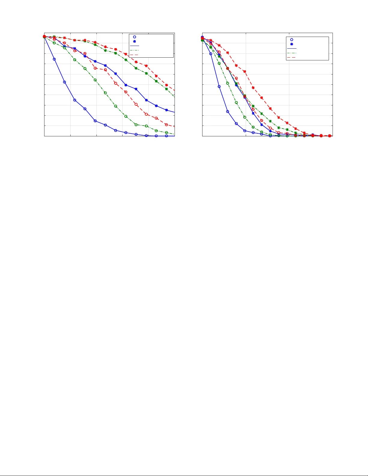
Adv ersarial T raining for Probabilistic Spiking Neural Networks Alireza Bagheri † ECE Department New J erse y Institute of T ec hnology New ark, NJ 07102, USA Email: ab 745@ nj it.edu Osv aldo Simeone † Department of Informatics King’ s Colle ge London London, WC2R 2LS, UK Email: osv aldo.simeone @ k cl.ac.uk Bipin Rajendran ECE Department New J erse y Institute of T ec hnology New ark, NJ 07102, USA Email: bipin @ nj it.edu Abstract —Classifiers trained using con ventional empirical risk minimization or maximum likelihood methods ar e known to suffer dramatic performance degradations when tested o ver examples adv ersarially selected based on knowledge of the clas- sifier’ s decision rule. Due to the prominence of Artificial Neural Networks (ANNs) as classifiers, their sensitivity to adversarial examples, as well as rob ust training schemes, hav e been recently the subject of intense in vestigation. In this paper , for the first time, the sensitivity of spiking neural networks (SNNs), or third-generation neural networks, to adversarial examples is studied. The study considers rate and time encoding, as well as rate and first-to-spike decoding. Furthermore, a robust training mechanism is proposed that is demonstrated to enhance the performance of SNNs under white-box attacks. Index T erms —Spiking Neural Networks (SNNs), adversarial examples, adversarial training, Generalized Linear Model (GLM) I . I N T RO D U C T I O N The classification accurac y of Artificial Neural Netw orks (ANNs) trained ov er large data sets from the problem domain has attained super-human lev els for many tasks including image identification [1]. Ne v ertheless, the performance of clas- sifiers trained using conv entional empirical risk minimization or Maximum Likelihood (ML) is known to decrease dramat- ically when ev aluated over examples adversarially selected based on knowledge of the classifier’ s decision rule [2]. T o mitigate this problem, robust training strategies that are aware of the presence of adversarial perturbations have been sho wn to improve the accuracy of classifiers, including ANNs, when tested ov er adversarial examples [2]–[4]. ANNs are kno wn to be energy-intensi ve, hindering their implementation on ener gy-limited processors such as mobile devices. Despite the recent industrial efforts around the pro- duction of more ener gy-efficient chips for ANNs [5], the gap between the ener gy efficienc y of the human brain and that of ANNs remains significant [6], [7]. A promising alternativ e paradigm is offered by Spiking Neural Networks (SNNs), in which synaptic input and neuronal output signals are sparse asynchronous binary spike trains [5]. Unlike ANNs, SNNs are hybrid digital-analog machines that make use of the temporal dimension, not just as a neutral substrate for computing, but as a means to encode and process information [7]. N X N Y 1 1 Ou tp u t lay er Inp u t lay er 1 1 T 1 T 1 T 1 T ΄ T ΄ 2 2 2 2 2 Fig. 1. T wo-layer SNN for supervised learning. T raining methods for SNNs typically assume deterministic non-linear dynamic models for the spiking neurons, and are either motiv ated by biological plausibility , such as the spike- timing-dependent plasticity (STDP) rule [5], [8], or by an attempt to mimic the operation of ANNs and associated learn- ing rules (see, e.g., [9] and references therein). Deterministic models are known to be limited in their expressi v e po wer , especially as it pertains prior domain kno wledge, uncertainty , and definition of generic queries and tasks. Training for probabilistic models of SNNs has recently been in vestigated in, e.g., [10]–[13] using ML and variational inference principles. In this paper , for the first time, the sensitivity of SNNs trained via ML is studied under white-box adversarial attacks, and a rob ust training mechanism is proposed that is demon- strated to enhance the performance of SNNs under adversarial examples. Specifically , we focus on a two-layer SNN (see Fig. 1), and consider rate and time encoding, as well as rate and first-to-spike decoding [13]. Our results illuminate the sensitivity of SNNs to adversarial example under different encoding and decoding schemes, and the ef fectiv eness of robust training methods. The rest of the paper is organized as follo ws. In Sec. II, we describe the architecture of the two-layer SNN with Gen- eralized Linear Model (GLM) neuron, as well as information encoding and decoding mechanisms. The design of adversarial perturbations is cov ered in Sec. III, while a rob ust training is presented in Sec. IV. Sec. V presents numerical results, and closing remarks are giv en in Sec. VI. I I . S N N - B A S E D C L A S S I F I C A T I O N In this section, we introduce the classification task and the SNN architecture under study . Network Ar chitecture : W e consider the problem of clas- sification using the two-layer SNN illustrated in Fig. 1. The SNN is fully connected and has N X presynaptic neurons in the input, or sensory layer , and N Y neurons in the output layer . Each output neuron is associated with a class. In order to feed the SNN, an input example, e.g., a gray scale image, is encoded into a set of N X discrete-time spike trains, each with T samples. The input spike trains are fed to the N Y postsynaptic GLM neurons, which output discrete-time spike trains. A decoder then selects the image class on the basis of the spike trains emitted by the output neurons. Information Encoding : W e consider two encoding mech- anisms. 1 ) Rate encoding : W ith the con ventional rate encoding method (see, e.g., [14]), each entry of the input signal is con verted into a discrete-time spike train by generating an independent and identically distributed (i.i.d.) Bernoulli vec- tor . The probability of generating a “1” , i.e., a spike, is proportional to the value of the entry . In the experiments in Sec. V, we use gray scale images of USPS dataset with pixel intensities normalized between 0 and 1 that yield a proportional spike probability between 0 and 1 / 2 . 2 ) T ime encoding : With the time encoding method, each entry of the input signal is con verted into a spike train ha ving only one spike, whose timing depends on the entry value. In particular , assuming intensity-to-latency encoding [14]–[16], the spike timing in the time interval [1 , T ] depends linearly on the entry value, such that the maximum v alue yields a spike at the first time sample t = 1 , and the minimum value is mapped to a spike in the last time sample t = T . GLM Neuron Model : The relationship between the input spike trains from the N X presynaptic neurons and the output spike train of any postsynaptic neuron i follo ws a Bernoulli GLM with canonical link function (see, e.g., [13], [17]). T o elaborate, we denote as x j,t and y i,t the binary signal emitted by the j -th presynaptic and the i -th postsynaptic neurons, respectiv ely , at time t . Also, we let x b j,a = ( x j,a , ..., x j,b ) be the vector of samples from spiking process of the presynaptic neuron j in the time interval [ a, b ] . Similarly , the vector y b i,a = ( y i,a , ..., y i,b ) contains samples from the spiking process of the neuron i in the interval [ a, b ] . The membrane potential of postsynaptic neuron i at time t is giv en by u i,t = N X X j =1 α T j,i x t − 1 j,t − τ y + β T i y t − 1 i,t − τ 0 y + γ i , (1) where α j,i ∈ R τ y is a vector that defines the synaptic kernel (SK) applied on the { j, i } synapse between presynaptic neuron j and postsynaptic neuron i ; β i ∈ R τ 0 y is the feedback kernel (FK); and γ i is a bias parameter . Note that τ y and τ 0 y denote the lengths of the SK and FK, respecti vely . The v ector of variable parameters θ i includes the bias γ i and the parameters that define the SK and FK filters, which are discussed below . According to the GLM, the log-probability of the output spike train y i = [ y i, 1 , ..., y i,T ] T conditioned on the input spike trains x = { x j } N X j =1 can be written as log p θ i ( y i | x ) = T X t =1 [ y i,t log g ( u i,t ) + ¯ y i,t log ¯ g ( u i,t )] , (2) where g ( · ) is an activ ation function, such as the sigmoid function g ( x ) = σ ( x ) = 1 / (1 + exp ( − x )) , and we defined ¯ y i,t = 1 − y i,t and ¯ g ( u i,t ) = 1 − g ( u i,t ) . As per (2), each sample y i,t is Bernoulli distributed with spiking probability g ( u i,t ) . As in [13], we adopt the parameterized model of [17] for the SK and FK filters. Accordingly , we write the SK α j,i and the FK β i as α j,i = K α X k =1 w j,i,k a k = Aw j,i , (3) and β i = K β X k =1 v i,k b k = Bv i , (4) respectiv ely , where we have defined the fix ed basis matrices A = [ a 1 , ..., a K α ] and B =  b 1 , ..., b K β  and the vectors w j,i = [ w j,i, 1 , ..., w j,i,K α ] T and v i =  v i, 1 , ..., v i,K β  T ; K α and K β denote the respectiv e number of basis functions; a k = [ a k, 1 , ..., a k,τ y ] T and b k = [ b k, 1 , ..., b k,τ 0 y ] T are the basis v ectors; and { w j,i,k } and { v i,k } are the learnable weights for the kernels α j,i and β i , respecti vely . For the experiments discussed in Sec. V, we adopt the raised cosine basis functions introduced in [17, Sec. Methods]. Information Decoding : W e also consider two alternativ e decoding methods, namely rate decoding and first-to-spike decoding. 1 ) Rate decoding : With rate decoding, decoding is carried out by selecting the output neuron with the largest number of spikes. 2 ) F irst-to-spik e decoding : W ith first-to- spike decoding, the class that corresponds to the neuron that spikes first is selected. ML training : Con ventional ML training is performed dif- ferently under rate and first-to-spike decoding methods, as briefly revie wed next. 1 ) Rate decoding : W ith rate decoding, the postsynaptic neuron corresponding to the correct label c ∈ { 1 , ..., N Y } is assigned a desired output spike train y c containing a number of spikes, while an all-zero vector y i , i 6 = c , is assigned to the other postsynaptic neurons. Using the ML criterion, one hence maximizes the sum of the log-probabilities (2) of the desired output spikes y ( c ) = { y 1 , ..., y N Y } for the given N X input spike trains x = { x 1 , ..., x N X } . The log-likelihood function for a giv en training example ( x , c ) can be written as L θ ( x , c ) = N Y X i =1 log p θ i ( y i | x ) , (5) where the parameter vector θ = { W , V , γ } includes the parameters W = { W i } N Y i =1 , V = { v i } N Y i =1 and γ = { γ i } N Y i =1 . The sum in (5) is further extended to all examples in the training set. The negati ve log-likelihood (NLL) − L θ is conv ex with respect to θ and can be minimized via SGD [13]. 2 ) Fir st-to-spike decoding : W ith first-to-spike decoding, the class that corresponds to the neuron that spikes first is selected. The ML criterion hence maximizes the probability to hav e the first spik e at the output neuron corresponding to the correct label. The logarithm of this probability for a gi ven example ( x , c ) can be written as L θ ( x , c ) = log T X t =1 p t ( θ ) ! , (6) where p t ( θ ) = N Y Y i =1 ,i 6 = c t Y t 0 =1 ¯ g ( u i,t 0 ) g ( u c,t ) t − 1 Y t 0 =1 ¯ g ( u c,t 0 ) , (7) is the probability of having the first spike at the correct neuron c at time t . In (7), the potential u i,t for all i is obtained from (1) by setting y i,t = 0 for all i and t . The minimization of the log-likelihood function L θ in (6), which is not conca ve, can be tackled via SGD as proposed in [13]. I I I . D E S I G N I N G A D V E R S A R I A L E X A M P L E S In this work, we consider white-box attacks based on full knowledge of the model, i.e., of the parameter vector θ , as well as of the encoding and decoding strategies. Accordingly , giv en an example ( x , c ) , an adversarial spike train x adv is obtained as a perturbed version of the original input x , where the perturbation is selected so as to cause the classifier to be more likely to predict an incorrect label c 0 6 = c , while being sufficiently small. W e consider the follo wing types of perturbations: ( i ) Re- move attack : one or more spikes are removed from the input x ; ( ii ) Add attack : one or more spikes are added to the input x ; and ( iii ) Flip attack : one or more spikes are added or removed. The size of the disturbance is measured for all attacks by the number of spikes that are added and/or removed. Mathemati- cally , this can be expressed as the Hamming distance d H  x , x adv  = N X X j =1 T X t =1 1  x j,t 6 = x adv j,t  , (8) where 1 ( · ) is the indicator function, i.e., 1 ( a ) = 1 if condition a is true and 1 ( a ) = 0 otherwise. In order to select the adv ersarial perturbation of an input x , we consider the maximization of the likelihood of a gi ven incorrect target class c 0 6 = c . According to [18], an ef fecti ve way to choose the tar get class c 0 is to find the class c LL 6 = c that is the least likely under the giv en model θ . Mathematically , for a giv en training example ( x , c ) , the least likely class is obtained by solving the problem c LL = argmin c 0 6 = c L θ ( x , c 0 ) , (9) where the log-likelihood L θ ( x , c 0 ) is gi ven by (5) for rate decoding and (6) for first-to-spike decoding. Algorithm 1 Greedy Design ( θ , T A ,  ) Input: x , θ , T A ,  1: Compute c LL from (9) 2: Initialize: x adv (0) ← x 3: f or i = 1 to b N X T c do 4: x adv ( i ) ← x adv ( i − 1) + p , where p is obtained by solving problem (10) with x adv ( i − 1) in lieu of x and p j,t = 0 for all t > T A . 5: end f or Output: x adv Algorithm 2 Adversarial T raining ( T A ,  A ) Input: T raining set, basis functions A and B , learning rate η , T A , and  A Initialize : θ 1: f or each iteration do 2: Choose example ( x , c ) from the training set 3: Compute x adv and c LL from Algorithm 1 with input θ , T A and  A 4: Update θ : θ ← θ + η ∇ θ L θ  x adv , c  5: end f or Output: θ Then, in order to compute the adversarial perturbation p , we maximize the likelihood of class c LL under model θ by tackling the following optimization problem max p ∈C L θ  x + p , c LL  s.t. k p k 0 ≤ N X T , (10) where k p k 0 denotes the number of non-zero elements of p . In (10), the perturbation  > 0 controls the adversary strength. In particular, the adversary is allowed to add or remov e spikes from a fraction  of the N X T input samples, i.e., T samples for each input neuron. The constraint set C in problem (10) is gi ven by the set of binary perturbations, i.e., C = { 0 , 1 } N X T , for add attacks, since spikes can only be added; C = { 0 , − 1 } N X T for remov e attacks; and C = { 0 , ± 1 } N X T for flip attacks. The exact solution of problem (10) requires an exhausti ve search ov er all possible perturbations of N X T samples. In the worst case of flip attacks, the resulting search space is hence exponential in N X and T . Therefore, here we resort to a greedy search method. As detailed in Algorithm 1, at each of the b N X T c steps, the method looks for the best spike to add, remove or flip, depending on the attack type. W e further reduce complexity by searching only among the first T A ≤ T samples across all input neurons. As a results, the complexity of each step of Algorithm 1 is at most N X T A . I V . R O B U S T T R A I N I N G In order to increase the robustness of the trained SNN to adversarial examples, in this section, we propose a robust training procedure. Accordingly , in a manner similar to [4], during the SGD-based training phase, each training example 0 0.00 2 0.00 4 0.00 6 0.00 8 0.01 0 .012 ǫ 0 10 20 30 40 50 60 70 80 90 100 T est Accur acy [%] Flip Add Remov e Rate Dec First-to-spike Dec Adver saria l Ran dom Fig. 2. T est accuracy for ML training under adversarial and random changes versus  with rate encoding for both rate and first-to-spike decoding rules ( T = K = 16) . ( x , c ) is substituted with the adversarial example x adv obtained from Algorithm 1 for the current iterate θ . The training algorithm is detailed in Algorithm 2. Note that, the robust training algorithm is parameterized by T A and  A , which determine the parameters of the assumed adversary during training. V . N U M E R I C A L R E S U LT S In this section, we numerically study the performance of the described probabilistic SNN under the adversarial attacks. W e use the standard USPS dataset as the input data. As a result, we have N X = 256 , with one input neuron per pixel of the 16 × 16 images. Unless stated otherwise, we focus solely in the classes { 1 , 5 , 7 , 9 } and we set T = K = 16 . W e assume the worst-case T A = T for the adversary during the test phase. For rate decoding, we use a desired spike train with one spike after ev ery three zeros. SGD is applied for 200 training epochs and early stopping is used for all schemes. Holdout validation with 20 % of training samples is applied to select between 10 − 3 and 10 − 4 for the constant learning rate η . The model parameters θ are randomly initialized with uniform distribution between -1 and 1. W e first e valuate the sensitivity of different encoding and de- coding schemes to adversarial examples obtained as explained in Sec. III. For reference, we consider also perturbations obtained by randomly and uniformly adding, removing and flipping spikes. Fig. 2 illustrates the test accuracy under ad- versarial and random perturbations when performing standard ML training. The accuracy is plotted versus the adversary’ s power  assuming rate encoding and both rate and first-to-spike decoding rules. The results highlight the notable difference in performance degradation caused by random perturbations and adversarial attacks. In particular , adversarial changes can cause a significant drop in classification accuracy e ven with small 0 0.00 2 0.00 4 0.00 6 0.00 8 0.01 0 .012 ǫ 0 10 20 30 40 50 60 70 80 90 100 T est Accur acy [%] Flip Add Remov e Rate Enc Time Enc Fig. 3. T est accuracy for ML training under adversarial attacks versus  with both rate and time encoding rules for first-to-spike decoding ( T = K = 16) . values of  , particularly when the most po werful flip attacks are used. First-to-spike decoding is seen to be more resistant to add and flip attacks, while it is more vulnerable than rate decoding to remov e spike attacks. The resilience of first-to- spike decoding can be interpreted as a consequence of the fact that the log-likelihood (6), unlike (5) for rate decoding, associates multiple outputs to the correct class, namely all of those with the correct neuron spiking first. Nevertheless, removing properly selected spikes can be more deleterious to first-to-spike decoding as it may prevent spiking by the correct neuron. The comparison between rate and time encoding in terms of sensitivity to adversarial e xamples is considered in Fig. 3 un- der the assumption of first-to-spike decoding. T ime encoding is seen to be significantly less resilient than rate encoding. This is due to the fact that time encoding, in the form considered here of intensity-to-latency encoding, which associated a single spike per input neuron [14], can be easily made ineffecti ve by removing selected spikes. W e then ev aluate the impact of rob ust adversarial training as compared to standard ML. T o this end, in Fig. 4, we plot the test accurac y for the case of flip and remove attacks for both ML and adversarial training when T = K = 8 . Here we also focus solely on the two classes { 5 , 7 } . W e recall that the adversarial training scheme is parametrized by the time support T A of the attacks considered during training, here T A = 8 , and by its power  A , here  A = 5 / 2048 and  A = 10 / 2048 . It is observed that robust training can signifi- cantly improv e the rob ustness of the SNN classifier , even when  A is not equal to the v alue  used by the attacker during the test phase. Furthermore, increasing  A enhances the robustness of the trained SNN at the cost of a higher computational complexity . For instance, for an attacker in the test phase 0 0.005 0.01 0.01 5 0.02 0.025 ǫ 0 10 20 30 40 50 60 70 80 90 100 T est Accur acy [%] Adv fl ip Adv remov e ML T r Adv T r (8, 5/2048) Adv T r (8, 10/2048) Fig. 4. T est accuracy under adversarial attacks versus  with rate encoding and rate decoding with ML and adv ersarial training ( T = K = 8) . with  = 10 / 2048 , i.e., with 10 bit flips, con ventional ML achiev es an accuracy of 45% , while adversarial training with  A = 10 / 2048 (i.e., 10 bit flips) achiev es an accuracy of 87% . Finally , the results show that the classifier remains resilient against other type of attacks, despite being trained assuming the flip attack. Finally , under the same conditions as in Fig. 5, we study the effect of limiting the po wer of the adversary assumed during training by considering T A = 1 and T A = 8 with the same  A = 5 / 2048 . W e assume time encoding and rate decoding. It is observed that rob ust training can still impro ve the rob ustness of the SNN classifier, ev en when T A  T during training. For instance, for an attacker in the test phase with  = 5 / 2048 , i.e., 5 bit flips, con ventional ML achieves an accuracy of 34 . 2% , while adv ersarial training with  A = 5 / 2048 and T A = 1 and 8 achie ves accuracy le vels of 60 . 3% and 77 . 5% , respecti vely . V I . C O N C L U S I O N S In this paper, we hav e studied for the first time the sensiti vity of a probabilistic two-layer SNN under adversarial perturba- tions. W e considered rate and time encoding, as well as rate and first-to-spike decoding. W e ha ve proposed mechanisms to build adv ersarial examples, as well as a robust training method that increases the resilience of the SNN. Additional work is needed in order to generalize the results to multi-layer networks. V I I . A C K N OW L E D G M E N T This work was supported by the U.S. NSF under grant ECCS # 1710009. O. Simeone has also receiv ed funding from the European Research Council (ERC) under the European Unions Horizon 2020 research and innov ation program (grant agreement # 725731). 0 0.00 5 0.01 0 .015 ǫ 0 10 20 30 40 50 60 70 80 90 100 T est Accur acy [%] Adv fl ip Adv remov e ML T r Adv T r (1, 5/2048) Adv T r (8, 5/2048) Fig. 5. T est accuracy under adversarial attacks versus  with time encoding and rate decoding with ML and adversarial training ( T = K = 8) . R E F E R E N C E S [1] R. Ranjan, S. Sankaranarayanan, A. Bansal, N. Bodla, J.-C. Chen, V . M. Patel, C. D. Castillo, and R. Chellappa, “Deep learning for understanding faces: Machines may be just as good, or better, than humans, ” IEEE Signal Pr ocess. Mag. , vol. 35, no. 1, pp. 66–83, 2018. [2] I. J. Goodfellow , J. Shlens, and C. Szegedy , “Explaining and harnessing adversarial examples, ” in Int. Conf. on Learn. Repr . (ICLR) , 2015. [3] A. Fawzi, S.-M. Moosavi-Dezfooli, and P . Frossard, “The robustness of deep networks: A geometrical perspectiv e, ” IEEE Signal Pr ocess. Mag. , vol. 34, no. 6, pp. 50–62, 2017. [4] A. Madry , A. Makelov , L. Schmidt, D. Tsipras, and A. Vladu, “T ow ards deep learning models resistant to adversarial attacks, ” arXiv pr eprint arXiv:1706.06083 , 2017. [5] H. Paugam-Moisy and S. Bohte, “Computing with spiking neuron networks, ” Handbook of natural computing , pp. 335–376, 2012. [6] J. V incent, “Intel investig ates chips designed like your brain to turn the AI tide, ” https://www .thever ge .com/2017/9/26/16365390/intel- in vestigates-chips-designed-like-your -brain-to-turn-the-ai-tide , Accessed: Sept. 26, 2017. [7] J. E. Smith, “Research agenda: Spacetime computation and the neocor- tex, ” IEEE Micro , vol. 37, no. 1, pp. 8–14, 2017. [8] F . Ponulak and A. Kasi ´ nski, “Supervised learning in spiking neural networks with ReSuMe: sequence learning, classification, and spik e shifting, ” Neural Comput , vol. 22, no. 2, pp. 467–510, 2010. [9] A. Sengupta, Y . Y e, R. W ang, C. Liu, and K. Roy , “Going deeper in spiking neural netw orks: VGG and residual architectures, ” arXiv pr eprint arXiv:1802.02627 , 2018. [10] B. Gardner and A. Gr ¨ uning, “Supervised learning in spiking neural networks for precise temporal encoding, ” PloS one , vol. 11, no. 8, pp. 1–28, 2016. [11] S. Guo, Z. Y u, F . Deng, X. Hu, and F . Chen, “Hierarchical bayesian inference and learning in spiking neural netw orks, ” IEEE T rans. Cybern. , vol. PP , no. 99, pp. 1–13, 2017. [12] D. J. Rezende, D. W ierstra, and W . Gerstner , “V ariational learning for recurrent spiking networks, ” Adv Neural Inf Pr ocess Syst , pp. 136–144, 2011. [13] A. Bagheri, O. Simeone, and B. Rajendran, “Training probabilistic spiking neural networks with first-to-spike decoding, ” arXiv pr eprint arXiv:1710.10704 , 2017. [14] E. Stromatias, M. Soto, T . Serrano-Gotarredona, and B. Linares- Barranco, “ An ev ent-driv en classifier for spiking neural networks fed with synthetic or dynamic vision sensor data, ” F r ont Neurosci , vol. 11, pp. 1–17, 2017. [15] T . Masquelier and S. J. Thorpe, “Unsupervised learning of visual features through spike timing dependent plasticity , ” PLoS Comput. Biol. , vol. 3, no. 2, pp. 247–257, 2007. [16] S. R. Kheradpisheh, M. Ganjtabesh, S. J. Thorpe, and T . Masquelier, “STDP-based spiking deep neural networks for object recognition, ” arXiv pr eprint arXiv:1611.01421 , 2016. [17] J. W . Pillow , J. Shlens, L. Paninski, A. Sher, A. M. Litke, E. Chichilnisky , and E. P . Simoncelli, “Spatio-temporal correlations and visual signaling in a complete neuronal population, ” Nature , vol. 454, no. 7207, p. 995, 2008. [18] A. Kurakin, I. Goodfellow , and S. Bengio, “ Adversarial examples in the physical world, ” arXiv preprint , 2016.