Understanding Deep Neural Networks with Rectified Linear Units
In this paper we investigate the family of functions representable by deep neural networks (DNN) with rectified linear units (ReLU). We give an algorithm to train a ReLU DNN with one hidden layer to *global optimality* with runtime polynomial in the …
Authors: Raman Arora, Amitabh Basu, Poorya Mianjy
Published as a conference paper at ICLR 2018 U N D E R S T A N D I N G D E E P N E U R A L N E T W O R K S W I T H R E C T I FI E D L I N E A R U N I T S Raman Arora ∗ Amitabh Basu † Poorya Mianjy ‡ Anirbit Mukherjee § Johns Hopkins Univ ersity A B S T R AC T In this paper we in vestigate the family of functions representable by deep neural networks (DNN) with rectified linear units (ReLU). W e giv e an algorithm to train a ReLU DNN with one hidden layer to global optimality with runtime polynomial in the data size albeit e xponential in the input dimension. Further , we improv e on the known lower bounds on size (from exponential to super e xponential) for approx- imating a ReLU deep net function by a shallower ReLU net. Our gap theorems hold for smoothly parametrized families of “hard” functions, contrary to count- able, discrete families kno wn in the literature. An example consequence of our gap theorems is the following: for every natural number k there exists a function representable by a ReLU DNN with k 2 hidden layers and total size k 3 , such that any ReLU DNN with at most k hidden layers will require at least 1 2 k k +1 − 1 total nodes. Finally , for the family of R n → R DNNs with ReLU acti vations, we sho w a new lowerbound on the number of affine pieces, which is lar ger than previous constructions in certain regimes of the network architecture and most distincti vely our lo werbound is demonstrated by an explicit construction of a smoothly par am- eterized family of functions attaining this scaling. Our construction utilizes the theory of zonotopes from polyhedral theory . 1 I N T RO D U C T I O N Deep neural networks (DNNs) provide an e xcellent family of hypotheses for machine learning tasks such as classification. Neural networks with a single hidden layer of finite size can represent any continuous function on a compact subset of R n arbitrary well. The uni versal approximation result was first gi ven by Cybenko in 1989 for sigmoidal activ ation function (Cybenko, 1989), and later generalized by Hornik to an arbitrary bounded and nonconstant activ ation function Hornik (1991). Furthermore, neural networks ha ve finite VC dimension (depending polynomially on the number of edges in the network), and therefore, are P A C (probably approximately correct) learnable using a sample of size that is polynomial in the size of the networks Anthony & Bartlett (1999). Howe ver , neural networks based methods were shown to be computationally hard to learn (Anthony & Bartlett, 1999) and had mixed empirical success. Consequently , DNNs fell out of fav or by late 90s. Recently , there has been a resurgence of DNNs with the advent of deep learning LeCun et al. (2015). Deep learning, loosely speaking, refers to a suite of computational techniques that hav e been dev el- oped recently for training DNNs. It started with the work of Hinton et al. (2006), which g ave empir- ical evidence that if DNNs are initialized properly (for instance, using unsupervised pre-training), then we can find good solutions in a reasonable amount of runtime. This w ork was soon follo wed by a series of early successes of deep learning at significantly improving the state-of-the-art in speech recognition Hinton et al. (2012). Since then, deep learning has received immense attention from the machine learning community with se veral state-of-the-art AI systems in speech recognition, im- age classification, and natural language processing based on deep neural nets Hinton et al. (2012); Dahl et al. (2013); Krizhevsk y et al. (2012); Le (2013); Sutske ver et al. (2014). While there is less of evidence now that pre-training actually helps, sev eral other solutions hav e since been put forth ∗ Department of Computer Science, Email: arora@cs.jhu.edu † Department of Applied Mathematics and Statistics, Email: basu.amitabh@jhu.edu ‡ Department of Computer Science, Email: mianjy@jhu.edu § Department of Applied Mathematics and Statistics, Email: amukhe14@jhu.edu 1 Published as a conference paper at ICLR 2018 to address the issue of ef ficiently training DNNs. These include heuristics such as dropouts Sri- vasta va et al. (2014), but also considering alternate deep architectures such as con volutional neural networks Sermanet et al. (2014), deep belief networks Hinton et al. (2006), and deep Boltzmann ma- chines Salakhutdino v & Hinton (2009). In addition, deep architectures based on ne w non-saturating activ ation functions have been suggested to be more ef fectively trainable – the most successful and widely popular of these is the rectified linear unit (ReLU) activ ation, i.e., σ ( x ) = max { 0 , x } , which is the focus of study in this paper . In this paper , we formally study deep neural networks with rectified linear units; we refer to these deep architectures as ReLU DNNs. Our work is inspired by these recent attempts to understand the reason behind the successes of deep learning, both in terms of the structure of the functions represented by DNNs, T elgarsky (2015; 2016); Kane & W illiams (2015); Shamir (2016), as well as efforts which hav e tried to understand the non-conv ex nature of the training problem of DNNs better Kawaguchi (2016); Haef fele & V idal (2015). Our in vestigation of the function space repre- sented by ReLU DNNs also takes inspiration from the classical theory of circuit complexity; we refer the reader to Arora & Barak (2009); Shpilka & Y ehudayof f (2010); Jukna (2012); Saptharishi (2014); Allender (1998) for various surve ys of this deep and fascinating field. In particular , our gap results are inspired by results like the ones by Hastad Hastad (1986), Razborov Razboro v (1987) and Smolensky Smolensky (1987) which show a strict separation of complexity classes. W e make progress tow ards similar statements with deep neural nets with ReLU activ ation. 1 . 1 N O TA T I O N A N D D E FI N I T I O N S W e extend the ReLU activ ation function to vectors x ∈ R n through entry-wise operation: σ ( x ) = (max { 0 , x 1 } , max { 0 , x 2 } , . . . , max { 0 , x n } ) . For any ( m, n ) ∈ N , let A n m and L n m denote the class of affine and linear transformations from R m → R n , respectiv ely . Definition 1. [ReLU DNNs, depth, width, size] For any number of hidden layers k ∈ N , input and output dimensions w 0 , w k +1 ∈ N , a R w 0 → R w k +1 ReLU DNN is given by specifying a sequence of k natural numbers w 1 , w 2 , . . . , w k representing widths of the hidden layers, a set of k af fine transformations T i : R w i − 1 → R w i for i = 1 , . . . , k and a linear transformation T k +1 : R w k → R w k +1 corresponding to weights of the hidden layers. Such a ReLU DNN is called a ( k + 1) -layer ReLU DNN, and is said to have k hidden layers. The function f : R n 1 → R n 2 computed or represented by this ReLU DNN is f = T k +1 ◦ σ ◦ T k ◦ · · · ◦ T 2 ◦ σ ◦ T 1 , (1.1) where ◦ denotes function composition. The depth of a ReLU DNN is defined as k + 1 . The width of a ReLU DNN is max { w 1 , . . . , w k } . The size of the ReLU DNN is w 1 + w 2 + . . . + w k . Definition 2. W e denote the class of R w 0 → R w k +1 ReLU DNNs with k hidden layers of widths { w i } k i =1 by F { w i } k +1 i =0 , i.e. F { w i } k +1 i =0 := { T k +1 ◦ σ ◦ T k ◦ · · · ◦ σ ◦ T 1 : T i ∈ A w i w i − 1 ∀ i ∈ { 1 , . . . , k } , T k +1 ∈ L w k +1 w k } (1.2) Definition 3. [Piecewise linear functions] W e say a function f : R n → R is continuous piecewise linear (PWL) if there exists a finite set of polyhedra whose union is R n , and f is affine linear over each polyhedron (note that the definition automatically implies continuity of the function because the affine regions are closed and cover R n , and affine functions are continuous). The number of pieces of f is the number of maximal connected subsets of R n ov er which f is affine linear (which is finite). Many of our important statements will be phrased in terms of the follo wing simplex. Definition 4. Let M > 0 be any positi ve real number and p ≥ 1 be an y natural number . Define the following set: ∆ p M := { x ∈ R p : 0 < x 1 < x 2 < . . . < x p < M } . 2 E X AC T C H A R A C T E R I Z A T I O N O F F U N C T I O N C L A S S R E P R E S E N T E D B Y R E L U D N N S One of the main advantages of DNNs is that they can represent a large family of functions with a relati vely small number of parameters. In this section, we giv e an exact characterization of the 2 Published as a conference paper at ICLR 2018 functions representable by ReLU DNNs. Moreo ver , we show how structural properties of ReLU DNNs, specifically their depth and width, affects their expressi ve power . It is clear from definition that any function from R n → R represented by a ReLU DNN is a continuous piecewise linear (PWL) function. In what follows, we show that the con verse is also true, that is any PWL function is representable by a ReLU DNN. In particular , the following theorem establishes a one-to-one correspondence between the class of ReLU DNNs and PWL functions. Theorem 2.1. Every R n → R ReLU DNN represents a piecewise linear function, and e very piece- wise linear function R n → R can be represented by a ReLU DNN with at most d log 2 ( n + 1) e + 1 depth. Proof Sketch: It is clear that any function represented by a ReLU DNN is a PWL function. T o see the con verse, we first note that any PWL function can be represented as a linear combination of piecewise linear con ve x functions. More formally , by Theorem 1 in (W ang & Sun, 2005), for every piecewise linear function f : R n → R , there exists a finite set of affine linear functions ` 1 , . . . , ` k and subsets S 1 , . . . , S p ⊆ { 1 , . . . , k } (not necessarily disjoint) where each S i is of cardinality at most n + 1 , such that f = p X j =1 s j max i ∈ S j ` i , (2.1) where s j ∈ {− 1 , +1 } for all j = 1 , . . . , p . Since a function of the form max i ∈ S j ` i is a piecewise linear con vex function with at most n + 1 pieces (because | S j | ≤ n + 1 ), Equation (2.1) says that any continuous piece wise linear function (not necessarily con ve x) can be obtained as a linear combination of piece wise linear con vex functions each of which has at most n + 1 affine pieces. Furthermore, Lemmas D.1, D.2 and D.3 in the Appendix (see supplementary material), show that composition, addition, and pointwise maximum of PWL functions are also representable by ReLU DNNs. In particular , in Lemma D.3 we note that max { x, y } = x + y 2 + | x − y | 2 is implementable by a two layer ReLU network and use this construction in an inducti ve manner to show that maximum of n + 1 numbers can be computed using a ReLU DNN with depth at most d log 2 ( n + 1) e . While Theorem 2.1 giv es an upper bound on the depth of the networks needed to represent all continuous piece wise linear functions on R n , it does not giv e any tight bounds on the size of the networks that are needed to represent a gi ven piecewise linear function. For n = 1 , we give tight bounds on size as follows: Theorem 2.2. Gi ven any piece wise linear function R → R with p pieces there exists a 2-layer DNN with at most p nodes that can represent f . Moreo ver , any 2-layer DNN that represents f has size at least p − 1 . Finally , the main result of this section follo ws from Theorem 2.1, and well-known facts that the piecewise linear functions are dense in the family of compactly supported continuous functions and the family of compactly supported continuous functions are dense in L q ( R n ) (Royden & Fitzpatrick, 2010)). Recall that L q ( R n ) is the space of Lebesgue integrable functions f such that R | f | q dµ < ∞ , where µ is the Lebesgue measure on R n (see Royden Royden & Fitzpatrick (2010)). Theorem 2.3. Every function in L q ( R n ) , (1 ≤ q ≤ ∞ ) can be arbitrarily well-approximated in the L q norm (which for a function f is gi ven by || f || q = ( R | f | q ) 1 /q ) by a ReLU DNN function with at most d log 2 ( n + 1) e hidden layers. Moreover , for n = 1 , any such L q function can be arbitrarily well-approximated by a 2-layer DNN, with tight bounds on the size of such a DNN in terms of the approximation. Proofs of Theorems 2.2 and 2.3 are pro vided in Appendix A. W e would like to remark that a weak er version of Theorem 2.1 was observed in (Goodfellow et al., 2013, Proposition 4.1) (with no bound on the depth), along with a univ ersal approximation theorem (Goodfello w et al., 2013, Theorem 4.3) similar to Theorem 2.3. The authors of Goodfellow et al. (2013) also used a pre vious result of W ang (W ang, 2004) for obtaining their result. In a subsequent w ork Boris Hanin (Hanin, 2017) has, among other things, found a width and depth upper bound for ReLU net representation of positi ve PWL functions on [0 , 1] n . The width upperbound is n+3 for general positi ve PWL functions and n + 1 for conv ex positiv e PWL functions. F or con vex positi ve PWL functions his depth upper bound is sharp if we disallow dead ReLUs. 3 Published as a conference paper at ICLR 2018 3 B E N E FI T S O F D E P T H Success of deep learning has been largely attributed to the depth of the networks, i.e. number of successiv e affine transformations followed by nonlinearities, which is shown to be extracting hierarchical features from the data. In contrast, traditional machine learning frameworks including support vector machines, generalized linear models, and k ernel machines can be seen as instances of shallow networks, where a linear transformation acts on a single layer of nonlinear feature extraction. In this section, we e xplore the importance of depth in ReLU DNNs. In particular , in Section 3.1, we provide a smoothly parametrized family of R → R “hard” functions representable by ReLU DNNs, which requires exponentially larger size for a shallower network. Furthermore, in Section 3.2, we construct a continuum of R n → R “hard” functions representable by ReLU DNNs, which to the best of our knowledge is the first explicit construction of ReLU DNN functions whose number of affine pieces grows exponentially with input dimension. The proofs of the theorems in this section are provided in Appendix B. 3 . 1 C I R C U I T L OW E R B O U N D S F O R R → R R E L U D N N S In this section, we are only concerned about R → R ReLU DNNs, i.e. both input and output dimensions are equal to one. The following theorem sho ws the depth-size trade-off in this setting. Theorem 3.1. For every pair of natural numbers k ≥ 1 , w ≥ 2 , there exists a family of hard functions representable by a R → R ( k + 1) -layer ReLU DNN of width w such that if it is also representable by a ( k 0 + 1) -layer ReLU DNN for any k 0 ≤ k , then this ( k 0 + 1) -layer ReLU DNN has size at least 1 2 k 0 w k k 0 − 1 . In fact our family of hard functions described abo ve has a very intricate structure as stated belo w . Theorem 3.2. F or e very k ≥ 1 , w ≥ 2 , every member of the family of hard functions in Theorem 3.1 has w k pieces and this family can be parametrized by [ M > 0 (∆ w − 1 M × ∆ w − 1 M × . . . × ∆ w − 1 M ) | {z } k times , (3.1) i.e., for ev ery point in the set above, there e xists a distinct function with the stated properties. The following is an immediate corollary of Theorem 3.1 by choosing the parameters carefully . Corollary 3.3. For every k ∈ N and > 0 , there is a family of functions defined on the real line such that ev ery function f from this family can be represented by a ( k 1+ ) + 1 -layer DNN with size k 2+ and if f is represented by a k + 1 -layer DNN, then this DNN must hav e size at least 1 2 k · k k − 1 . Moreov er, this f amily can be parametrized as, ∪ M > 0 ∆ k 2+ − 1 M . A particularly illuminativ e special case is obtained by setting = 1 in Corollary 3.3: Corollary 3.4. For e very natural number k ∈ N , there is a f amily of functions parameterized by the set ∪ M > 0 ∆ k 3 − 1 M such that any f from this family can be represented by a k 2 + 1 -layer DNN with k 3 nodes, and ev ery k + 1 -layer DNN that represents f needs at least 1 2 k k +1 − 1 nodes. W e can also get hardness of approximation versions of Theorem 3.1 and Corollaries 3.3 and 3.4, with the same gaps (upto constant terms), using the follo wing theorem. Theorem 3.5. For every k ≥ 1 , w ≥ 2 , there exists a function f k,w that can be represented by a ( k + 1) -layer ReLU DNN with w nodes in each layer , such that for all δ > 0 and k 0 ≤ k the following holds: inf g ∈G k 0 ,δ Z 1 x =0 | f k,w ( x ) − g ( x ) | dx > δ, where G k 0 ,δ is the family of functions representable by ReLU DNNs with depth at most k 0 + 1 , and size at most k 0 w k/k 0 (1 − 4 δ ) 1 /k 0 2 1+1 /k 0 . The depth-size trade-off results in Theorems 3.1, and 3.5 extend and improv e T elgarsky’ s theorems from (T elgarsky, 2015; 2016) in the follo wing three ways: 4 Published as a conference paper at ICLR 2018 (i) If we use our Theorem 3.5 to the pair of neural nets considered by T elgarsky in Theorem 1 . 1 in T elgarsky (2016) which are at depths k 3 (of size also scaling as k 3 ) and k then for this purpose of approximation in the ` 1 − norm we would get a size lower bound for the shallower net which scales as Ω(2 k 2 ) which is exponentially (in depth) larger than the lower bound of Ω(2 k ) that T elgarsky can get for this scenario. (ii) T elgarsky’ s family of hard functions is parameterized by a single natural number k . In contrast, we show that for every pair of natural numbers w and k , and a point from the set in equation 3.1, there exists a “hard” function which to be represented by a depth k 0 network would need a size of at least w k k 0 k 0 . W ith the extra fle xibility of choosing the parameter w , for the purpose of sho wing gaps in representation ability of deep nets we can shows size lower bounds which are super -exponential in depth as explained in Corollaries 3.3 and 3.4. (iii) A characteristic feature of the “hard” functions in Boolean circuit comple xity is that the y are usually a countable family of functions and not a “smooth” family of hard functions. In fact, in the last section of T elgarsky (2015), T elgarsky states this as a “weakness” of the state-of-the-art results on “hard” functions for both Boolean circuit complexity and neural nets research. In contrast, we provide a smoothly parameterized f amily of “hard” functions in Section 3.1 (parametrized by the set in equation 3.1). Such a continuum of hard functions wasn’ t demonstrated before this work. W e point out that T elgarsk y’ s results in (T elgarsky, 2016) apply to deep neural nets with a host of different acti vation functions, whereas, our results are specifically for neural nets with rectified linear units. In this sense, T elgarsky’ s results from (T elgarsky, 2016) are more general than our results in this paper , but with weaker gap guarantees. Eldan-Shamir (Shamir, 2016; Eldan & Shamir, 2016) show that there exists an R n → R function that can be represented by a 3-layer DNN, that takes exponential in n number of nodes to be approximated to within some constant by a 2-layer DNN. While their results are not immediately comparable with T elgarsky’ s or our results, it is an interesting open question to e xtend their results to a constant depth hierarch y statement analogous to the recent result of Rossman et al (Rossman et al., 2015). W e also note that in last few years, there has been much effort in the community to show size lowerbounds on ReLU DNNs trying to approximate various classes of functions which are themselves not necessarily exactly representable by ReLU DNNs (Y arotsk y, 2016; Liang & Srikant, 2016; Safran & Shamir, 2017). 3 . 2 A C O N T I N U U M O F H A R D F U N C T I O N S F O R R n → R F O R n ≥ 2 One measure of complexity of a family of R n → R “hard” functions represented by ReLU DNNs is the asymptotics of the number of pieces as a function of dimension n , depth k + 1 and size s of the ReLU DNNs. More precisely , suppose one has a family H of functions such that for e very n, k , w ∈ N the family contains at least one R n → R function representable by a ReLU DNN with depth at most k + 1 and maximum width at most w . The following definition formalizes a notion of complexity for such a H . Definition 5 (comp H ( n, k , w ) ) . The measure comp H ( n, k , w ) is defined as the maximum number of pieces (see Definition 3) of a R n → R function from H that can be represented by a ReLU DNN with depth at most k + 1 and maximum width at most w . Similar measures have been studied in previous works Montufar et al. (2014); Pascanu et al. (2013); Raghu et al. (2016). The best known families H are the ones from Theorem 4 of (Mont- ufar et al., 2014) and a mild generalization of Theorem 1 . 1 of (T elgarsky, 2016) to k layers of ReLU activ ations with width w ; these constructions achie ve b ( w n ) c ( k − 1) n ( P n j =0 w j ) and comp H ( n, k , s ) = O ( w k ) , respecti vely . At the end of this section we would explain the precise sense in which we improve on these numbers. An analysis of this comple xity measure is done using integer programming techniques in (Serra et al., 2017). Definition 6. Let b 1 , . . . , b m ∈ R n . The zonotope formed by b 1 , . . . , b m ∈ R n is defined as Z ( b 1 , . . . , b m ) := { λ 1 b 1 + . . . + λ m b m : − 1 ≤ λ i ≤ 1 , i = 1 , . . . , m } . 5 Published as a conference paper at ICLR 2018 (a) H 1 2 , 1 2 ◦ N ` 1 (b) H 1 2 , 1 2 ◦ γ Z ( b 1 , b 2 , b 3 , b 4 ) (c) H 1 2 , 1 2 , 1 2 ◦ γ Z ( b 1 , b 2 , b 3 , b 4 ) Figure 1: W e fix the a vectors for a two hidden layer R → R hard function as a 1 = a 2 = ( 1 2 ) ∈ ∆ 1 1 Left: A specific hard function induced by ` 1 norm: ZONOTOPE 2 2 , 2 , 2 [ a 1 , a 2 , b 1 , b 2 ] where b 1 = (0 , 1) and b 2 = (1 , 0) . Note that in this case the function can be seen as a composi- tion of H a 1 , a 2 with ` 1 -norm N ` 1 ( x ) := k x k 1 = γ Z ((0 , 1) , (1 , 0)) . Middle: A typical hard function ZONOTOPE 2 2 , 2 , 4 [ a 1 , a 2 , c 1 , c 2 , c 3 , c 4 ] with generators c 1 = ( 1 4 , 1 2 ) , c 2 = ( − 1 2 , 0) , c 3 = (0 , − 1 4 ) and c 4 = ( − 1 4 , − 1 4 ) . Note how increasing the number of zonotope generators makes the function more complex. Right: A harder function from ZONOTOPE 2 3 , 2 , 4 family with the same set of gen- erators c 1 , c 2 , c 3 , c 4 but one more hidden layer ( k = 3) . Note how increasing the depth make the function more complex. (For illustrative purposes we plot only the part of the function which lies abov e zero.) The set of vertices of Z ( b 1 , . . . , b m ) will be denoted by vert( Z ( b 1 , . . . , b m )) . The support func- tion γ Z ( b 1 ,..., b m ) : R n → R associated with the zonotope Z ( b 1 , . . . , b m ) is defined as γ Z ( b 1 ,..., b m ) ( r ) = max x ∈ Z ( b 1 ,..., b m ) h r , x i . The following results are well-kno wn in the theory of zonotopes (Ziegler, 1995). Theorem 3.6. The following are all true. 1. | vert( Z ( b 1 , . . . , b m )) | ≤ P n − 1 i =0 m − 1 i . The set of ( b 1 , . . . , b m ) ∈ R n × . . . × R n such that this does not hold at equality is a 0 measure set. 2. γ Z ( b 1 ,..., b m ) ( r ) = max x ∈ Z ( b 1 ,..., b m ) h r , x i = max x ∈ vert( Z ( b 1 ,..., b m )) h r , x i , and γ Z ( b 1 ,..., b m ) is therefore a piecewise linear function with | v ert( Z ( b 1 , . . . , b m )) | pieces. 3. γ Z ( b 1 ,..., b m ) ( r ) = |h r , b 1 i| + . . . + |h r , b m i| . Definition 7 (extremal zonotope set) . The set S ( n, m ) will denote the set of ( b 1 , . . . , b m ) ∈ R n × . . . × R n such that | v ert( Z ( b 1 , . . . , b m )) | = P n − 1 i =0 m − 1 i . S ( n, m ) is the so-called “extremal zonotope set”, which is a subset of R nm , whose complement has zero Lebesgue measure in R nm . Lemma 3.7. Giv en any b 1 , . . . , b m ∈ R n , there exists a 2-layer ReLU DNN with size 2 m which represents the function γ Z ( b 1 ,..., b m ) ( r ) . Definition 8. For p ∈ N and a ∈ ∆ p M , we define a function h a : R → R which is piecewise linear ov er the segments ( −∞ , 0] , [0 , a 1 ] , [ a 1 , a 2 ] , . . . , [ a p , M ] , [ M , + ∞ ) defined as follows: h a ( x ) = 0 for all x ≤ 0 , h a ( a i ) = M ( i mo d 2) , and h a ( M ) = M − h a ( a p ) and for x ≥ M , h a ( x ) is a linear continuation of the piece o ver the interv al [ a p , M ] . Note that the function has p + 2 pieces, with the leftmost piece ha ving slope 0 . Furthermore, for a 1 , . . . , a k ∈ ∆ p M , we denote the composition of the functions h a 1 , h a 2 , . . . , h a k by H a 1 ,..., a k := h a k ◦ h a k − 1 ◦ . . . ◦ h a 1 . Proposition 3.8. Giv en any tuple ( b 1 , . . . , b m ) ∈ S ( n, m ) and an y point ( a 1 , . . . , a k ) ∈ [ M > 0 (∆ w − 1 M × ∆ w − 1 M × . . . × ∆ w − 1 M ) | {z } k times , the function ZONOTOPE n k,w ,m [ a 1 , . . . , a k , b 1 , . . . , b m ] := H a 1 ,..., a k ◦ γ Z ( b 1 ,..., b m ) has ( m − 1) n − 1 w k pieces and it can be represented by a k + 2 layer ReLU DNN with size 2 m + w k . 6 Published as a conference paper at ICLR 2018 Finally , we are ready to state the main result of this section. Theorem 3.9. For every tuple of natural numbers n, k , m ≥ 1 and w ≥ 2 , there exists a family of R n → R functions, which we call ZONOTOPE n k,w ,m with the following properties: (i) Every f ∈ ZONOTOPE n k,w ,m is representable by a ReLU DNN of depth k + 2 and size 2 m + w k , and has P n − 1 i =0 m − 1 i w k pieces. (ii) Consider any f ∈ ZONOTOPE n k,w ,m . If f is represented by a ( k 0 + 1) - layer DNN for any k 0 ≤ k , then this ( k 0 + 1) -layer DNN has size at least max 1 2 ( k 0 w k k 0 n ) · ( m − 1) (1 − 1 n ) 1 k 0 − 1 , w k k 0 n 1 /k 0 k 0 . (iii) The family ZONOTOPE n k,w ,m is in one-to-one correspondence with S ( n, m ) × [ M > 0 (∆ w − 1 M × ∆ w − 1 M × . . . × ∆ w − 1 M ) | {z } k times . Comparison to the results in (Montufar et al., 2014) F irstly we note that the construction in (Montufar et al., 2014) requires all the hidden layers to ha ve width at least as big as the input dimensionality n . In contrast, we do not impose such restrictions and the network size in our construction is independent of the input dimensionality . Thus our result probes networks with bottleneck architectures whose complexity cant be seen from their result. Secondly , in terms of our complexity measure, there seem to be regimes where our bound does better . One such regime, for example, is when n ≤ w < 2 n and k ∈ Ω( n log( n ) ) , by setting in our construction m < n . Thir dly , it is not clear to us whether the construction in (Montufar et al., 2014) giv es a smoothly parameterized family of functions other than by introducing small perturbations of the construc- tion in their paper . In contrast, we hav e a smoothly parameterized family which is in one-to-one correspondence with a well-understood manifold like the higher -dimensional torus. 4 T R A I N I N G 2 - L AY E R R n → R R E L U D N N S T O G L O B A L O P T I M A L I T Y In this section we consider the follo wing empirical risk minimization problem. Giv en D data points ( x i , y i ) ∈ R n × R , i = 1 , . . . , D , find the function f represented by 2-layer R n → R ReLU DNNs of width w , that minimizes the following optimization problem min f ∈F { n,w, 1 } 1 D D X i =1 ` ( f ( x i ) , y i ) ≡ min T 1 ∈A w n , T 2 ∈L 1 w 1 D D X i =1 ` T 2 ( σ ( T 1 ( x i ))) , y i (4.1) where ` : R × R → R is a con vex loss function (common loss functions are the squared loss, ` ( y , y 0 ) = ( y − y 0 ) 2 , and the hinge loss function giv en by ` ( y , y 0 ) = max { 0 , 1 − y y 0 } ). Our main result of this section gives an algorithm to solve the above empirical risk minimization problem to global optimality . Theorem 4.1. There exists an algorithm to find a global optimum of Problem 4.1 in time O (2 w ( D ) nw poly ( D , n, w )) . Note that the running time O (2 w ( D ) nw poly ( D , n, w )) is polynomial in the data size D for fixed n, w . Proof Sketch: A full proof of Theorem 4.1 is included in Appendix C. Here we provide a sketch of the proof. When the empirical risk minimization problem is vie wed as an optimization problem in the space of weights of the ReLU DNN, it is a nonconv ex, quadratic problem. Howe ver , one can instead search ov er the space of functions representable by 2-layer DNNs by writing them in the form similar to (2.1). This breaks the problem into tw o parts: a combinatorial search and then a con vex problem that is essentially linear regression with linear inequality constraints. This enables us to guarantee global optimality . 7 Published as a conference paper at ICLR 2018 Algorithm 1 Empirical Risk Minimization 1: function ERM( D ) Where D = { ( x i , y i ) } D i =1 ⊂ R n × R 2: S = { +1 , − 1 } w All possible instantiations of top layer weights 3: P i = { ( P i + , P i − ) } , i = 1 , . . . , w All possible partitions of data into tw o parts 4: P = P 1 × P 2 × · · · × P w 5: count = 1 Counter 6: for s ∈ S do 7: for { ( P i + , P i − ) } w i =1 ∈ P do 8: loss(count) = minimize: ˜ a, ˜ b D X j =1 X i : j ∈ P i + ( s i (˜ a i · x j + ˜ b i ) , y j ) subject to: ˜ a i · x j + ˜ b i ≤ 0 ∀ j ∈ P i − ˜ a i · x j + ˜ b i ≥ 0 ∀ j ∈ P i + 9: count + + 10: end for 11: OPT = argmin loss(count) 12: end for 13: return { ˜ a } , { ˜ b } , s corresponding to OPT’s iterate 14: end function Let T 1 ( x ) = Ax + b and T 2 ( y ) = a 0 · y for A ∈ R w × n and b, a 0 ∈ R w . If we denote the i -th ro w of the matrix A by a i , and write b i , a 0 i to denote the i -th coordinates of the vectors b, a 0 respectiv ely , due to homogeneity of ReLU gates, the network output can be represented as f ( x ) = w X i =1 a 0 i max { 0 , a i · x + b i } = w X i =1 s i max { 0 , ˜ a i · x + ˜ b i } . where ˜ a i ∈ R n , ˜ b i ∈ R and s i ∈ {− 1 , +1 } for all i = 1 , . . . , w . For any hidden node i ∈ { 1 . . . , w } , the pair ( ˜ a i , ˜ b i ) induces a partition P i := ( P i + , P i − ) on the dataset, gi ven by P i − = { j : ˜ a i · x j + ˜ b i ≤ 0 } and P i + = { 1 , . . . , D }\ P i − . Algorithm 1 proceeds by generating all combinations of the partitions P i as well as the top layer weights s ∈ { +1 , − 1 } w , and minimizing the loss P D j =1 P i : j ∈ P i + ` ( s i (˜ a i · x j + ˜ b i ) , y j ) subject to the constraints ˜ a i · x j + ˜ b i ≤ 0 ∀ j ∈ P i − and ˜ a i · x j + ˜ b i ≥ 0 ∀ j ∈ P i + which are imposed for all i = 1 , . . . , w , which is a con vex program. Algorithm 1 implements the empirical risk minimization (ERM) rule for training ReLU DNN with one hidden layer . T o the best of our knowledge there is no other known algorithm that solves the ERM problem to global optimality . W e note that due to kno wn hardness results exponential dependence on the input dimension is unav oidable Blum & Riv est (1992); Shalev-Shwartz & Ben- David (2014); Algorithm 1 runs in time polynomial in the number of data points. T o the best of our knowledge there is no hardness result known which rules out empirical risk minimization of deep nets in time polynomial in circuit size or data size. Thus our training result is a step towards resolving this gap in the complexity literature. A related result for impr operly learning ReLUs has been recently obtained by Goel et al (Goel et al., 2016). In contrast, our algorithm returns a ReLU DNN from the class being learned. Another difference is that their result considers the notion of r eliable learning as opposed to the empirical risk minimization objectiv e considered in (4.1). 5 D I S C U S S I O N The running time of the algorithm that we gi ve in this work to find the e xact global minima of a two layer ReLU-DNN is exponential in the input dimension n and the number of hidden nodes w . The exponential dependence on n can not be removed unless P = N P ; see Shalev-Shwartz & Ben-David (2014); Blum & Riv est (1992); DasGupta et al. (1995). Howe ver , we are not aware of any complexity results which would rule out the possibility of an algorithm which trains to global optimality in time that is polynomial in the data size and/or the number of hidden nodes, assuming that the input dimension is a fixed constant. Resolving this dependence on network size would be another step to wards clarifying the theoretical complexity of training ReLU DNNs and is a good 8 Published as a conference paper at ICLR 2018 open question for future research, in our opinion. Perhaps an ev en better breakthrough would be to get optimal training algorithms for DNNs with two or more hidden layers and this seems like a substantially harder nut to crack. It would also be a significant breakthrough to get gap results between consecutiv e constant depths or between logarithmic and constant depths. A C K N O W L E D G M E N T S W e would lik e to thank Christian Tjandraatmadja for pointing out a subtle error in a pre vious v ersion of the paper , which affected the comple xity results for the number of linear regions in our construc- tions in Section 3.2. Anirbit would like to thank Ramprasad Saptharishi, Piyush Sriv astav a and Rohit Gurjar for e xtensiv e discussions on Boolean and arithmetic circuit complexity . This paper has been immensely influenced by the perspectiv es gained during those extremely helpful discussions. Amitabh Basu gratefully ackno wledges support from the NSF grant CMMI1452820. Raman Arora was supported in part by NSF BIGD A T A grant IIS-1546482. R E F E R E N C E S Eric Allender . Complexity theory lecture notes. https://www.cs.rutgers.edu/ ˜ allender/lecture.notes/ , 1998. Martin Anthony and Peter L. Bartlett. Neural network learning: Theoretical foundations . Cam- bridge Univ ersity Press, 1999. Sanjeev Arora and Boaz Barak. Computational comple xity: a modern appr oach . Cambridge Uni- versity Press, 2009. A vrim L. Blum and Ronald L. Rivest. Training a 3-node neural network is np-complete. Neur al Networks , 5(1):117–127, 1992. George Cybenko. Approximation by superpositions of a sigmoidal function. Mathematics of contr ol, signals and systems , 2(4):303–314, 1989. George E. Dahl, T ara N. Sainath, and Geof frey E. Hinton. Improving deep neural networks for lvcsr using rectified linear units and dropout. In 2013 IEEE International Confer ence on Acoustics, Speech and Signal Pr ocessing , pp. 8609–8613. IEEE, 2013. Bhaskar DasGupta, Ha va T . Siegelmann, and Eduardo Sontag. On the complexity of training neural networks with continuous activ ation functions. IEEE T ransactions on Neural Networks , 6(6): 1490–1504, 1995. Ronen Eldan and Ohad Shamir . The power of depth for feedforward neural networks. In 29th Annual Confer ence on Learning Theory , pp. 907–940, 2016. Surbhi Goel, V arun Kanade, Adam Kliv ans, and Justin Thaler . Reliably learning the relu in polyno- mial time. arXiv preprint , 2016. Ian J Goodfellow , Da vid W arde-Farley , Mehdi Mirza, Aaron Courville, and Y oshua Bengio. Maxout networks. arXiv preprint , 2013. Benjamin D. Haef fele and Ren ´ e V idal. Global optimality in tensor factorization, deep learning, and beyond. arXiv pr eprint arXiv:1506.07540 , 2015. Boris Hanin. Uni versal function approximation by deep neural nets with bounded width and relu activ ations. arXiv preprint , 2017. Johan Hastad. Almost optimal lo wer bounds for small depth circuits. In Proceedings of the eigh- teenth annual A CM symposium on Theory of computing , pp. 6–20. ACM, 1986. Geoffre y Hinton, Li Deng, Dong Y u, George E. Dahl, Abdel-rahman Mohamed, Navdeep Jaitly , Andrew Senior , V incent V anhoucke, Patrick Nguyen, T ara N Sainath, et al. Deep neural netw orks for acoustic modeling in speech recognition: The shared vie ws of four research groups. IEEE Signal Pr ocessing Magazine , 29(6):82–97, 2012. Geoffre y E. Hinton, Simon Osindero, and Y ee-Whye T eh. A fast learning algorithm for deep belief nets. Neural computation , 18(7):1527–1554, 2006. Kurt Hornik. Approximation capabilities of multilayer feedforward networks. Neural networks , 4 (2):251–257, 1991. 9 Published as a conference paper at ICLR 2018 Stasys Jukna. Boolean function complexity: advances and fr ontiers , volume 27. Springer Science & Business Media, 2012. Daniel M. Kane and Ryan Williams. Super -linear gate and super -quadratic wire lo wer bounds for depth-two and depth-three threshold circuits. arXiv preprint , 2015. Kenji Kaw aguchi. Deep learning without poor local minima. arXiv pr eprint arXiv:1605.07110 , 2016. Alex Krizhe vsky , Ilya Sutskev er, and Geof frey E. Hinton. Imagenet classification with deep conv o- lutional neural networks. In Advances in neural information pr ocessing systems , pp. 1097–1105, 2012. Quoc V . Le. Building high-level features using large scale unsupervised learning. In 2013 IEEE international confer ence on acoustics, speech and signal pr ocessing , pp. 8595–8598. IEEE, 2013. Y ann LeCun, Y oshua Bengio, and Geof frey Hinton. Deep learning. Natur e , 521(7553):436–444, 2015. Shiyu Liang and R Srikant. Why deep neural networks for function approximation? 2016. Jiri Matousek. Lectur es on discrete geometry , v olume 212. Springer Science & Business Media, 2002. Guido F . Montufar , Razvan Pascanu, K yunghyun Cho, and Y oshua Bengio. On the number of linear regions of deep neural networks. In Advances in neural information processing systems , pp. 2924–2932, 2014. Razvan P ascanu, Guido Montufar , and Y oshua Bengio. On the number of response regions of deep feed forward networks with piece-wise linear activ ations. arXiv preprint , 2013. Maithra Raghu, Ben Poole, Jon Kleinberg, Surya Ganguli, and Jascha Sohl-Dickstein. On the ex- pressiv e power of deep neural netw orks. arXiv preprint , 2016. Alexander A. Razborov . Lower bounds on the size of bounded depth circuits over a complete basis with logical addition. Mathematical Notes , 41(4):333–338, 1987. Benjamin Rossman, Rocco A. Servedio, and Li-Y ang T an. An av erage-case depth hierarchy theo- rem for boolean circuits. In F oundations of Computer Science (FOCS), 2015 IEEE 56th Annual Symposium on , pp. 1030–1048. IEEE, 2015. H.L. Royden and P .M. Fitzpatrick. Real Analysis . Prentice Hall, 2010. Itay Safran and Ohad Shamir . Depth-width tradeof fs in approximating natural functions with neural networks. In International Conference on Mac hine Learning , pp. 2979–2987, 2017. Ruslan Salakhutdino v and Geof frey E. Hinton. Deep boltzmann machines. In International Confer- ence on Artificial Intelligence and Statistics (AIST ATS) , v olume 1, pp. 3, 2009. R. Saptharishi. A survey of lo wer bounds in arithmetic circuit complexity , 2014. Pierre Sermanet, Da vid Eigen, Xiang Zhang, Michael Mathieu, Rob Fergus, and Y ann LeCun. Over- feat: Inte grated recognition, localization and detection using conv olutional networks. In Interna- tional Conference on Learning Repr esentations (ICLR 2014) . arXiv preprint arXi v:1312.6229, 2014. Thiago Serra, Christian Tjandraatmadja, and Srikumar Ramalingam. Bounding and counting linear regions of deep neural networks. arXiv pr eprint arXiv:1711.02114 , 2017. Shai Shalev-Shwartz and Shai Ben-David. Understanding machine learning: F r om theory to algo- rithms . Cambridge university press, 2014. Ohad Shamir . Distribution-specific hardness of learning neural networks. arXiv pr eprint arXiv:1609.01037 , 2016. Amir Shpilka and Amir Y ehudayoff. Arithmetic circuits: A survey of recent results and open ques- tions. F oundations and T rends R in Theor etical Computer Science , 5(3–4):207–388, 2010. Roman Smolensky . Algebraic methods in the theory of lo wer bounds for boolean circuit complexity . In Pr oceedings of the nineteenth annual ACM symposium on Theory of computing , pp. 77–82. A CM, 1987. Nitish Sriv astava, Geoffre y E. Hinton, Alex Krizhevsk y , Ilya Sutske ver , and Ruslan Salakhutdinov . Dropout: a simple way to pre vent neural netw orks from o verfitting. Journal of Machine Learning Resear ch , 15(1):1929–1958, 2014. 10 Published as a conference paper at ICLR 2018 Ilya Sutske ver , Oriol V inyals, and Quoc V . Le. Sequence to sequence learning with neural netw orks. In Advances in neural information pr ocessing systems , pp. 3104–3112, 2014. Matus T elgarsk y . Representation benefits of deep feedforward networks. arXiv pr eprint arXiv:1509.08101 , 2015. Matus T elgarsky . benefits of depth in neural networks. In 29th Annual Confer ence on Learning Theory , pp. 1517–1539, 2016. Shuning W ang. General constructiv e representations for continuous piecewise-linear functions. IEEE T ransactions on Cir cuits and Systems I: Regular P apers , 51(9):1889–1896, 2004. Shuning W ang and Xusheng Sun. Generalization of hinging hyperplanes. IEEE T ransactions on Information Theory , 51(12):4425–4431, 2005. Dmitry Y arotsky . Error bounds for approximations with deep relu networks. arXiv preprint arXiv:1610.01145 , 2016. G ¨ unter M. Ziegler . Lectur es on polytopes , volume 152. Springer Science & Business Media, 1995. A E X P R E S S I N G P I E C E W I S E L I N E A R F U N C T I O N S U S I N G R E L U D N N S Pr oof of Theor em 2.2. Any continuous piece wise li near function R → R which has m pieces can be specified by three pieces of information, (1) s L the slope of the left most piece, (2) the coordinates of the non-differentiable points specified by a ( m − 1) − tuple { ( a i , b i ) } m − 1 i =1 (index ed from left to right) and (3) s R the slope of the rightmost piece. A tuple ( s L , s R , ( a 1 , b 1 ) , . . . , ( a m − 1 , b m − 1 ) uniquely specifies a m piecewise linear function from R → R and vice versa. Given such a tuple, we construct a 2 -layer DNN which computes the same piecewise linear function. One notes that for any a, r ∈ R , the function f ( x ) = 0 x ≤ a r ( x − a ) x > a (A.1) is equal to sgn( r ) max {| r | ( x − a ) , 0 } , which can be implemented by a 2-layer ReLU DNN with size 1. Similarly , any function of the form, g ( x ) = t ( x − a ) x ≤ a 0 x > a (A.2) is equal to − sgn( t ) max {−| t | ( x − a ) , 0 } , which can be implemented by a 2-layer ReLU DNN with size 1. The parameters r, t will be called the slopes of the function, and a will be called the br eakpoint of the function.If we can write the given piece wise linear function as a sum of m functions of the form (A.1) and (A.2), then by Lemma D.2 we would be done. It turns out that such a decomposition of any p piece PWL function h : R → R as a sum of p flaps can always be arranged where the breakpoints of the p flaps all are all contained in the p − 1 breakpoints of h . First, observe that adding a constant to a function does not change the complexity of the ReLU DNN expressing it, since this corresponds to a bias on the output node. Thus, we will assume that the v alue of h at the last break point a m − 1 is b m − 1 = 0 . W e no w use a single function f of the form (A.1) with slope r and breakpoint a = a m − 1 , and m − 1 functions g 1 , . . . , g m − 1 of the form (A.2) with slopes t 1 , . . . , t m − 1 and breakpoints a 1 , . . . , a m − 1 , respecti vely . Thus, we wish to e xpress h = f + g 1 + . . . + g m − 1 . Such a decomposition of h would be valid if we can find values for r , t 1 , . . . , t m − 1 such that (1) the slope of the above sum is = s L for x < a 1 , (2) the slope of the above sum is = s R for x > a m − 1 , and (3) for each i ∈ { 1 , 2 , 3 , .., m − 1 } we have b i = f ( a i ) + g 1 ( a i ) + . . . + g m − 1 ( a i ) . The abov e corresponds to asking for the existence of a solution to the follo wing set of simultaneous linear equations in r , t 1 , . . . , t m − 1 : s R = r , s L = t 1 + t 2 + . . . + t m − 1 , b i = m − 1 X j = i +1 t j ( a j − 1 − a j ) for all i = 1 , . . . , m − 2 It is easy to verify that the abov e set of simultaneous linear equations has a unique solution. Indeed, r must equal s R , and then one can solve for t 1 , . . . , t m − 1 starting from the last equation b m − 2 = 11 Published as a conference paper at ICLR 2018 t m − 1 ( a m − 2 − a m − 1 ) and then back substitute to compute t m − 2 , t m − 3 , . . . , t 1 . The lower bound of p − 1 on the size for any 2 -layer ReLU DNN that expresses a p piece function follows from Lemma D.6. One can do better in terms of size when the rightmost piece of the gi ven function is flat, i.e., s R = 0 . In this case r = 0 , which means that f = 0 ; thus, the decomposition of h above is of size p − 1 . A similar construction can be done when s L = 0 . This gives the follo wing statement which will be useful for constructing our forthcoming hard functions. Corollary A.1. If the rightmost or leftmost piece of a R → R piece wise linear function has 0 slope, then we can compute such a p piece function using a 2 -layer DNN with size p − 1 . Pr oof of theor em 2.3. Since any piece wise linear function R n → R is representable by a ReLU DNN by Corollary 2.1, the proof simply follo ws from the fact that the family of continuous piece- wise linear functions is dense in any L p ( R n ) space, for 1 ≤ p ≤ ∞ . B B E N E FI T S O F D E P T H B . 1 C O N S T R U C T I N G A C O N T I N U U M O F H A R D F U N C T I O N S F O R R → R R E L U D N N S A T E V E RY D E P T H A N D E V E RY W I D T H Lemma B.1. F or any M > 0 , p ∈ N , k ∈ N and a 1 , . . . , a k ∈ ∆ p M , if we compose the functions h a 1 , h a 2 , . . . , h a k the resulting function is a piecewise linear function with at most ( p + 1) k + 2 pieces, i.e., H a 1 ,..., a k := h a k ◦ h a k − 1 ◦ . . . ◦ h a 1 is piecewise linear with at most ( p + 1) k + 2 pieces, with ( p + 1) k of these pieces in the range [0 , M ] (see Figure 2). Moreo ver , in each piece in the range [0 , M ] , the function is affine with minimum value 0 and maximum value M . Pr oof. Simple induction on k . Pr oof of Theor em 3.2. Giv en k ≥ 1 and w ≥ 2 , choose any point ( a 1 , . . . , a k ) ∈ [ M > 0 (∆ w − 1 M × ∆ w − 1 M × . . . × ∆ w − 1 M ) | {z } k times . By Definition 8, each h a i , i = 1 , . . . , k is a piece wise linear function with w + 1 pieces and the leftmost piece having slope 0 . Thus, by Corollary A.1, each h a i , i = 1 , . . . , k can be represented by a 2-layer ReLU DNN with size w . Using Lemma D.1, H a 1 ,..., a k can be represented by a k + 1 layer DNN with size w k ; in fact, each hidden layer has exactly w nodes. Pr oof of Theor em 3.1. Follo ws from Theorem 3.2 and Lemma D.6. Pr oof of Theor em 3.5. Giv en k ≥ 1 and w ≥ 2 define q := w k and s q := h a ◦ h a ◦ . . . ◦ h a | {z } k times where a = ( 1 w , 2 w , . . . , w − 1 w ) ∈ ∆ q − 1 1 . Thus, s q is representable by a ReLU DNN of width w + 1 and depth k + 1 by Lemma D.1. In what follows, we want to gi ve a lo wer bound on the ` 1 distance of s q from any continuous p -piecewise linear comparator g p : R → R . The function s q contains b q 2 c triangles of width 2 q and unit height. A p -piece wise linear function has p − 1 breakpoints in the interv al [0 , 1] . So that in at least b w k 2 c − ( p − 1) triangles, g p has to be af fine. In the follo wing we demonstrate that 12 Published as a conference paper at ICLR 2018 -0.2 0 0.2 0.4 0.6 0.8 1 1.2 0 0.2 0.4 0.6 0.8 1 -0.2 0 0.2 0.4 0.6 0.8 1 1.2 0 0.2 0.4 0.6 0.8 1 -0.2 0 0.2 0.4 0.6 0.8 1 1.2 0 0.2 0.4 0.6 0.8 1 Figure 2: T op: h a 1 with a 1 ∈ ∆ 2 1 with 3 pieces in the range [0 , 1] . Middle: h a 2 with a 2 ∈ ∆ 1 1 with 2 pieces in the range [0 , 1] . Bottom: H a 1 , a 2 = h a 2 ◦ h a 1 with 2 · 3 = 6 pieces in the range [0 , 1] . The dotted line in the bottom panel corresponds to the function in the top panel. It shows that for ev ery piece of the dotted graph, there is a full copy of the graph in the middle panel. inside any triangle of s q , any af fine function will incur an ` 1 error of at least 1 2 w k . Z 2 i +2 w k x = 2 i w k | s q ( x ) − g p ( x ) | dx = Z 2 w k x =0 s q ( x ) − ( y 1 + ( x − 0) · y 2 − y 1 2 w k − 0 ) dx = Z 1 w k x =0 xw k − y 1 − w k x 2 ( y 2 − y 1 ) dx + Z 2 w k x = 1 w k 2 − xw k − y 1 − w k x 2 ( y 2 − y 1 ) dx = 1 w k Z 1 z =0 z − y 1 − z 2 ( y 2 − y 1 ) dz + 1 w k Z 2 z =1 2 − z − y 1 − z 2 ( y 2 − y 1 ) dz = 1 w k − 3 + y 1 + 2 y 2 1 2 + y 1 − y 2 + y 2 + 2( − 2 + y 1 ) 2 2 − y 1 + y 2 The abov e integral attains its minimum of 1 2 w k at y 1 = y 2 = 1 2 . Putting together, k s w k − g p k 1 ≥ b w k 2 c − ( p − 1) · 1 2 w k ≥ w k − 1 − 2( p − 1) 4 w k = 1 4 − 2 p − 1 4 w k Thus, for any δ > 0 , p ≤ w k − 4 w k δ + 1 2 = ⇒ 2 p − 1 ≤ ( 1 4 − δ )4 w k = ⇒ 1 4 − 2 p − 1 4 w k ≥ δ = ⇒ k s w k − g p k 1 ≥ δ. The result now follo ws from Lemma D.6. B . 2 A C O N T I N U U M O F H A R D F U N C T I O N S F O R R n → R F O R n ≥ 2 Pr oof of Lemma 3.7. By Theorem 3.6 part 3., γ Z ( b 1 ,..., b m ) ( r ) = |h r , b 1 i| + . . . + |h r , b m i| . It suffices to observ e |h r , b 1 i| + . . . + |h r , b m i| = max {h r , b 1 i , −h r , b 1 i} + . . . + max {h r , b m i , −h r , b m i} . Pr oof of Pr oposition 3.8. The fact that ZONOTOPE n k,w ,m [ a 1 , . . . , a k , b 1 , . . . , b m ] can be repre- sented by a k + 2 layer ReLU DNN with size 2 m + w k follows from Lemmas 3.7 and D.1. The number of pieces follo ws from the fact that γ Z ( b 1 ,..., b m ) has P n − 1 i =0 m − 1 i distinct linear pieces by parts 1. and 2. of Theorem 3.6, and H a 1 ,..., a k has w k pieces by Lemma B.1. Pr oof of Theor em 3.9. Follo ws from Proposition 3.8. 13 Published as a conference paper at ICLR 2018 C E X AC T E M P I R I C A L R I S K M I N I M I Z A T I O N Pr oof of Theor em 4.1. Let ` : R → R be an y con vex loss function, and let ( x 1 , y 1 ) , . . . , ( x D , y D ) ∈ R n × R be the gi ven D data points. As stated in (4.1), the problem requires us to find an af fine transformation T 1 : R n → R w and a linear transformation T 2 : R w → R , so as to minimize the empirical loss as stated in (4.1). Note that T 1 is given by a matrix A ∈ R w × n and a vector b ∈ R w so that T ( x ) = Ax + b for all x ∈ R n . Similarly , T 2 can be represented by a vector a 0 ∈ R w such that T 2 ( y ) = a 0 · y for all y ∈ R w . If we denote the i -th row of the matrix A by a i , and write b i , a 0 i to denote the i -th coordinates of the vectors b, a 0 respectiv ely , we can write the function represented by this network as f ( x ) = w X i =1 a 0 i max { 0 , a i · x + b i } = w X i =1 sgn( a 0 i ) max { 0 , ( | a 0 i | a i ) · x + | a 0 i | b i } . In other words, the family of functions o ver which we are searching is of the form f ( x ) = w X i =1 s i max { 0 , ˜ a i · x + ˜ b i } (C.1) where ˜ a i ∈ R n , b i ∈ R and s i ∈ {− 1 , +1 } for all i = 1 , . . . , w . W e now make the following observation. For a gi ven data point ( x j , y j ) if ˜ a i · x j + ˜ b i ≤ 0 , then the i -th term of (C.1) does not contribute to the loss function for this data point ( x j , y j ) . Thus, for every data point ( x j , y j ) , there exists a set S j ⊆ { 1 , . . . , w } such that f ( x j ) = P i ∈ S j s i (˜ a i · x j + ˜ b i ) . In particular , if we are giv en the set S j for ( x j , y j ) , then the expression on the right hand side of (C.1) reduces to a linear function of ˜ a i , ˜ b i . For any fixed i ∈ { 1 , . . . , w } , these sets S j induce a partition of the data set into two parts. In particular , we define P i + := { j : i ∈ S j } and P i − := { 1 , . . . , D } \ P i + . Observe now that this partition is also induced by the hyperplane gi ven by ˜ a i , ˜ b i : P i + = { j : ˜ a i · x j + ˜ b i > 0 } and P i + = { j : ˜ a i · x j + ˜ b i ≤ 0 } . Our strategy will be to guess the partitions P i + , P i − for each i = 1 , . . . , w , and then do linear regression with the constraint that regression’ s decision variables ˜ a i , ˜ b i induce the guessed partition. More formally , the algorithm does the following. For each i = 1 , . . . , w , the algorithm guesses a partition of the data set ( x j , y j ) , j = 1 , . . . , D by a h yperplane. Let us label the partitions as follo ws ( P i + , P i − ) , i = 1 , . . . , w . So, for each i = 1 , . . . , w , P i + ∪ P i − = { 1 , . . . , D } , P i + and P i − are disjoint, and there exists a vector c ∈ R n and a real number δ such that P i − = { j : c · x j + δ ≤ 0 } and P i + = { j : c · x j + δ > 0 } . Further, for each i = 1 , . . . , w the algorithm selects a vector s in { +1 , − 1 } w . For a fixed selection of partitions ( P i + , P i − ) , i = 1 , . . . , w and a vector s in { +1 , − 1 } w , the algorithm solves the following con vex optimization problem with decision variables ˜ a i ∈ R n , ˜ b i ∈ R for i = 1 , . . . , w (thus, we hav e a total of ( n + 1) · w decision variables). The feasible region of the optimization is giv en by the constraints ˜ a i · x j + ˜ b i ≤ 0 ∀ j ∈ P i − ˜ a i · x j + ˜ b i ≥ 0 ∀ j ∈ P i + (C.2) which are imposed for all i = 1 , . . . , w . Thus, we have a total of D · w constraints. Subject to these constraints we minimize the objective P D j =1 P i : j ∈ P i + ` ( s i (˜ a i · x j + ˜ b i ) , y j ) . Assuming the loss function ` is a con vex function in the first argument, the above objective is a con vex function. Thus, we hav e to minize a con vex objecti ve subject to the linear inequality constraints from (C.2). W e finally ha ve to count ho w many possible partitions ( P i + , P i − ) and vectors s the algorithm has to search through. It is well-known Matousek (2002) that the total number of possible hyperplane partitions of a set of size D in R n is at most 2 D n ≤ D n whenev er n ≥ 2 . Thus with a guess for each i = 1 , . . . , w , we hav e a total of at most D nw partitions. There are 2 w vectors s in {− 1 , +1 } w . This giv es us a total of 2 w D nw guesses for the partitions ( P i + , P i − ) and vectors s . For each such guess, we have a con vex optimization problem with ( n + 1) · w decision variables and D · w constraints, which can be solved in time poly ( D , n, w ) . Putting ev erything together , we have the running time claimed in the statement. 14 Published as a conference paper at ICLR 2018 The above argument holds only for n ≥ 2 , since we used the inequality 2 D n ≤ D n which only holds for n ≥ 2 . For n = 1 , a similar algorithm can be designed, but one which uses the characterization achieved in Theorem 2.2. Let ` : R → R be any con vex loss function, and let ( x 1 , y 1 ) , . . . , ( x D , y D ) ∈ R 2 be the given D data points. Using Theorem 2.2, to solv e problem (4.1) it suffices to find a R → R piecewise linear function f with w pieces that minimizes the total loss. In other words, the optimization problem (4.1) is equi valent to the problem min ( D X i =1 ` ( f ( x i ) , y i ) : f is piecewise linear with w pieces ) . (C.3) W e now use the observ ation that fitting piecewise linear functions to minimize loss is just a step away from linear regression, which is a special case where the function is contrained to hav e exactly one affine linear piece. Our algorithm will first guess the optimal partition of the data points such that all points in the same class of the partition correspond to the same af fine piece of f , and then do linear regression in each class of the partition. Altenativ ely , one can think of this as guessing the interval ( x i , x i +1 ) of data points where the w − 1 breakpoints of the piecewise linear function will lie, and then doing linear regression between the breakpoints. More formally , we parametrize piecewise linear functions with w pieces by the w slope-intercept values ( a 1 , b 1 ) , . . . , ( a 2 , b 2 ) , . . . , ( a w , b w ) of the w dif ferent pieces. This means that between break- points j and j + 1 , 1 ≤ j ≤ w − 2 , the function is gi ven by f ( x ) = a j +1 x + b j +1 , and the first and last pieces are a 1 x + b 1 and a w x + b w , respectiv ely . Define I to be the set of all ( w − 1) -tuples ( i 1 , . . . , i w − 1 ) of natural numbers such that 1 ≤ i 1 ≤ . . . ≤ i w − 1 ≤ D . Gi ven a fixed tuple I = ( i 1 , . . . , i w − 1 ) ∈ I , we wish to search through all piece- wise linear functions whose breakpoints, in order, appear in the interv als ( x i 1 , x i 1 +1 ) , ( x i 2 , x i 2 +1 ) , . . . , ( x i w − 1 , x i w − 1 +1 ) . Define also S = {− 1 , 1 } w − 1 . Any S ∈ S will have the following inter - pretation: if S j = 1 then a j ≤ a j +1 , and if S j = − 1 then a j ≥ a j +1 . No w for e very I ∈ I and S ∈ S , requiring a piecewise linear function that respects the conditions imposed by I and S is easily seen to be equiv alent to imposing the following linear inequalities on the parameters ( a 1 , b 1 ) , . . . , ( a 2 , b 2 ) , . . . , ( a w , b w ) : S j ( b j +1 − b j − ( a j − a j +1 ) x i j ) ≥ 0 S j ( b j +1 − b j − ( a j − a j +1 ) x i j +1 ) ≤ 0 S j ( a j +1 − a j ) ≥ 0 (C.4) Let the set of piecewise linear functions whose breakpoints satisfy the above be denoted by PWL 1 I ,S for I ∈ I , S ∈ S . Giv en a particular I ∈ I , we define D 1 := { x i : i ≤ i 1 } , D j := { x i : i j − 1 < i ≤ i 1 } j = 2 , . . . , w − 1 , D w := { x i : i > i w − 1 } . Observe that min { D X i =1 ` ( f ( x i ) − y i ) : f ∈ PWL 1 I ,S } = min { w X j =1 X i ∈ D j ` ( a j · x i + b j − y i ) : ( a j , b j ) satisfy (C.4) } (C.5) The right hand side of the above equation is the problem of minimizing a con ve x objecti ve subject to linear constraints. Now , to solve (C.3), we need to simply solv e the problem (C.5) for all I ∈ I , S ∈ S and pick the minimum. Since |I | = D w = O ( D w ) and |S | = 2 w − 1 we need to solve O (2 w · D w ) con vex optimization problems, each taking time O ( poly ( D )) . Therefore, the total running time is O ((2 D ) w poly ( D )) . 15 Published as a conference paper at ICLR 2018 D A U X I L I A RY L E M M A S Now we will collect some straightforward observations that will be used often. The following oper - ations preserve the property of being representable by a ReLU DNN. Lemma D.1. [Function Composition] If f 1 : R d → R m is represented by a d, m ReLU DNN with depth k 1 + 1 and size s 1 , and f 2 : R m → R n is represented by an m, n ReLU DNN with depth k 2 + 1 and size s 2 , then f 2 ◦ f 1 can be represented by a d, n ReLU DNN with depth k 1 + k 2 + 1 and size s 1 + s 2 . Pr oof. Follo ws from (1.1) and the fact that a composition of af fine transformations is another af fine transformation. Lemma D.2. [Function Addition] If f 1 : R n → R m is represented by a n, m ReLU DNN with depth k + 1 and size s 1 , and f 2 : R n → R m is represented by a n, m ReLU DNN with depth k + 1 and size s 2 , then f 1 + f 2 can be represented by a n, m ReLU DNN with depth k + 1 and size s 1 + s 2 . Pr oof. W e simply put the two ReLU DNNs in parallel and combine the appropriate coordinates of the outputs. Lemma D.3. [T aking maximums/minimums] Let f 1 , . . . , f m : R n → R be functions that can each be represented by R n → R ReLU DNNs with depths k i + 1 and size s i , i = 1 , . . . , m . Then the function f : R n → R defined as f ( x ) := max { f 1 ( x ) , . . . , f m ( x ) } can be represented by a ReLU DNN of depth at most max { k 1 , . . . , k m } + log( m ) + 1 and size at most s 1 + . . . s m + 4(2 m − 1) . Similarly , the function g ( x ) := min { f 1 ( x ) , . . . , f m ( x ) } can be represented by a ReLU DNN of depth at most max { k 1 , . . . , k m } + d log ( m ) e + 1 and size at most s 1 + . . . s m + 4(2 m − 1) . Pr oof. W e prov e this by induction on m . The base case m = 1 is trivial. For m ≥ 2 , consider g 1 := max { f 1 , . . . , f b m 2 c } and g 2 := max { f b m 2 c +1 , . . . , f m } . By the induction hypothesis (since b m 2 c , d m 2 e < m when m ≥ 2 ), g 1 and g 2 can be represented by ReLU DNNs of depths at most max { k 1 , . . . , k b m 2 c } + d log( b m 2 c ) e + 1 and max { k b m 2 c +1 , . . . , k m } + d log( d m 2 e ) e + 1 respectively , and sizes at most s 1 + . . . s b m 2 c + 4(2 b m 2 c − 1) and s b m 2 c +1 + . . . + s m + 4(2 b m 2 c − 1) , respecti vely . Therefore, the function G : R n → R 2 giv en by G ( x ) = ( g 1 ( x ) , g 2 ( x )) can be implemented by a ReLU DNN with depth at most max { k 1 , . . . , k m } + d log( d m 2 e ) e + 1 and size at most s 1 + . . . + s m + 4(2 m − 2) . W e now show how to represent the function T : R 2 → R defined as T ( x, y ) = max { x, y } = x + y 2 + | x − y | 2 by a 2-layer ReLU DNN with size 4 – see Figure 3. The result now follows from the fact that f = T ◦ G and Lemma D.1. Input x 1 Input x 2 x 1 + x 2 2 + | x 1 − x 2 | 2 1 1 -1 -1 -1 1 1 -1 1 2 − 1 2 1 2 1 2 Figure 3: A 2-layer ReLU DNN computing max { x 1 , x 2 } = x 1 + x 2 2 + | x 1 − x 2 | 2 Lemma D .4. Any af fine transformation T : R n → R m is representable by a 2-layer ReLU DNN of size 2 m . 16 Published as a conference paper at ICLR 2018 Pr oof. Simply use the fact that T = ( I ◦ σ ◦ T ) + ( − I ◦ σ ◦ ( − T )) , and the right hand side can be represented by a 2-layer ReLU DNN of size 2 m using Lemma D.2. Lemma D.5. Let f : R → R be a function represented by a R → R ReLU DNN with depth k + 1 and widths w 1 , . . . , w k of the k hidden layers. Then f is a PWL function with at most 2 k − 1 · ( w 1 + 1) · w 2 · . . . · w k pieces. -0.2 0 0.2 0.4 0.6 0.8 1 1.2 0 0.2 0.4 0.6 0.8 1 -0.2 0 0.2 0.4 0.6 0.8 1 1.2 -0.4 -0.2 0 0.2 0.4 0.6 Figure 4: The number of pieces increasing after activ ation. If the blue function is f , then the red function g = max { 0 , f + b } has at most twice the number of pieces as f for any bias b ∈ R . Pr oof. W e pro ve this by induction on k . The base case is k = 1 , i.e, we hav e a 2-layer ReLU DNN. Since e very acti vation node can produce at most one breakpoint in the piece wise linear function, we can get at most w 1 breakpoints, i.e., w 1 + 1 pieces. Now for the induction step, assume that for some k ≥ 1 , any R → R ReLU DNN with depth k + 1 and widths w 1 , . . . , w k of the k hidden layers produces at most 2 k − 1 · ( w 1 + 1) · w 2 · . . . · w k pieces. Consider any R → R ReLU DNN with depth k + 2 and widths w 1 , . . . , w k +1 of the k + 1 hidden layers. Observe that the input to any node in the last layer is the output of a R → R ReLU DNN with depth k + 1 and widths w 1 , . . . , w k . By the induction hypothesis, the input to this node in the last layer is a piece wise linear function f with at most 2 k − 1 · ( w 1 + 1) · w 2 · . . . · w k pieces. When we apply the activ ation, the new function g ( x ) = max { 0 , f ( x ) } , which is the output of this node, may hav e at most twice the number of pieces as f , because each original piece may be intersected by the x -axis; see Figure 4. Thus, after going through the layer , we take an affine combination of w k +1 functions, each with at most 2 · (2 k − 1 · ( w 1 + 1) · w 2 · . . . · w k ) pieces. In all, we can therefore get at most 2 · (2 k − 1 · ( w 1 + 1) · w 2 · . . . · w k ) · w k +1 pieces, which is equal to 2 k · ( w 1 + 1) · w 2 · . . . · w k · w k +1 , and the induction step is completed. Lemma D.5 has the follo wing consequence about the depth and size tradeoffs for expressing func- tions with agiv en number of pieces. Lemma D.6. Let f : R → R be a piece wise linear function with p pieces. If f is represented by a ReLU DNN with depth k + 1 , then it must hav e size at least 1 2 k p 1 /k − 1 . Con versely , any piecewise linear function f that represented by a ReLU DNN of depth k + 1 and size at most s , can ha ve at most ( 2 s k ) k pieces. Pr oof. Let widths of the k hidden layers be w 1 , . . . , w k . By Lemma D.5, we must have 2 k − 1 · ( w 1 + 1) · w 2 · . . . · w k ≥ p. (D.1) By the AM-GM inequality , minimizing the size w 1 + w 2 + . . . + w k subject to (D.1), means setting w 1 + 1 = w 2 = . . . = w k . This implies that w 1 + 1 = w 2 = . . . = w k ≥ 1 2 p 1 /k . The first statement follo ws. The second statement follo ws using the AM-GM inequality again, this time with a restriction on w 1 + w 2 + . . . + w k . 17
Original Paper
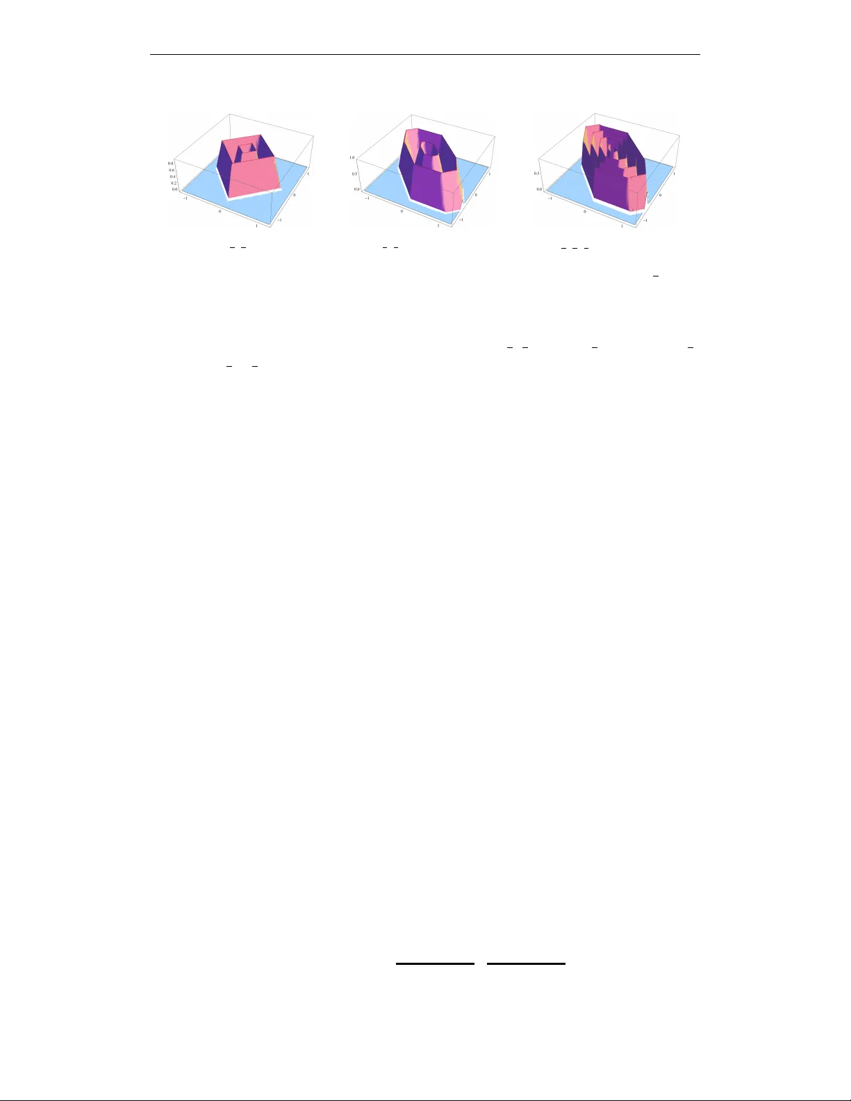
Loading high-quality paper...
Comments & Academic Discussion
Loading comments...
Leave a Comment