Age-Minimal Online Policies for Energy Harvesting Sensors with Incremental Battery Recharges

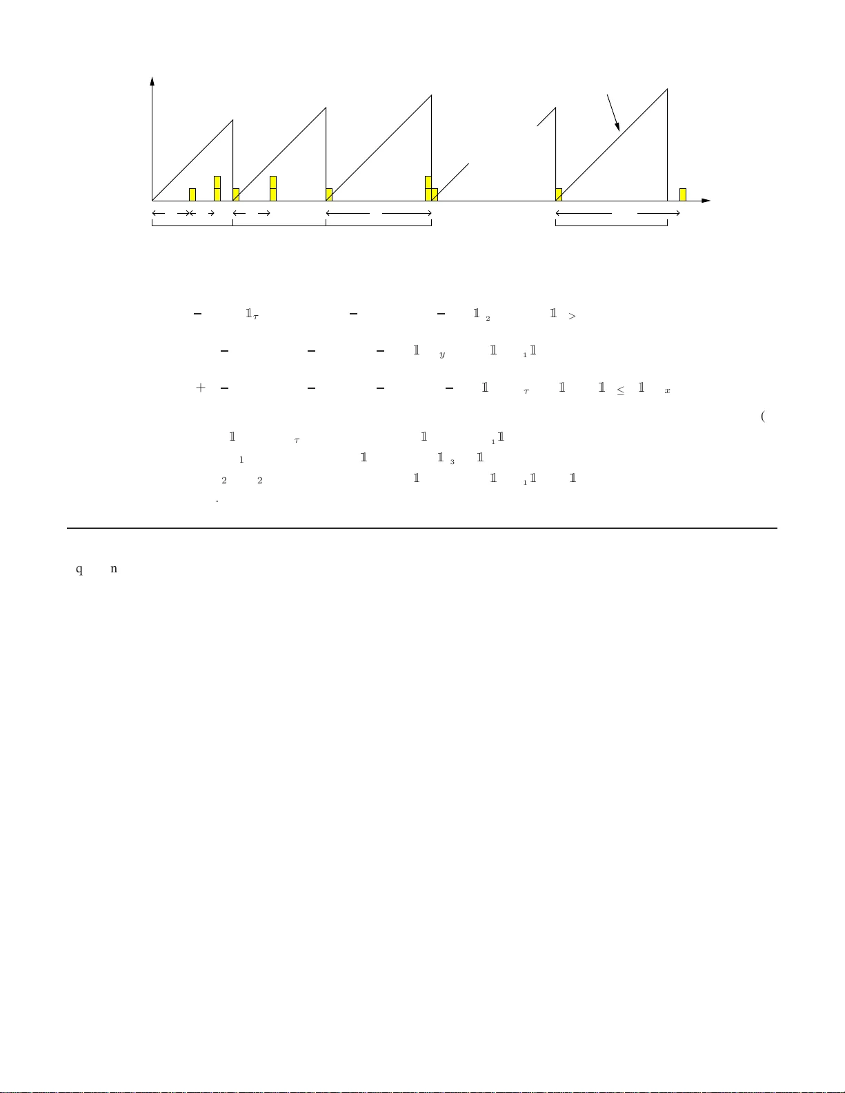
Age-Minimal Online Policies for En er gy Harve sting Sensors with Incremental Battery Rechar ges Ahmed Arafa 1 , Jing Y ang 2 , Senn ur Ulukus 3 , and H. V i ncen t Poo r 1 1 Electrical Engineer ing Department, Princeton Uni versity 2 School of Electrical Engin e ering and Computer Science , Penn sylvania State Un i versity 3 Departmen t of Electrical and Computer Engine ering, University of Marylan d Abstract — A sensor node th at is sendin g mea surement up- dates regarding some physical phenomenon to a destination is considered. The sen sor relies on energy harves ted from nature to transmit its updates, and is equip ped with a finite B -si zed battery to sa ve its harvested energ y . Energ y recharges the battery incr ementally in un i ts, according to a Poisson process, and one update consumes one energy unit to reach the d estination. The setting i s online, where th e energy arrival times are rev ealed causally after the energy is harvested. The goal is to up date the destin ation in a ti mely manner , namely , such that th e long term av erage ag e of information is minimized, subject to en ergy causality constraint s. The age of information at a given ti me is defined as the time spent since the latest update has reached the destination. It i s shown that the optimal update policy follows a r enewal structure, wher e the inter-update ti mes are independent, and the time durations between an y two consecutive events of submitting an u pdate and ha ving k uni ts of energy remaining in the battery are i n dependent and identi cally distributed for a giv en k ≤ B − 1 . The optimal renewal policy for th e case of B = 2 energy u nits is explicitl y characterized, and it is shown that it has an ener gy-dep endent thr eshold structure, where th e sensor updates only if the age gro ws above a certain th reshold that is a function of the amount of energy in its battery . I . I N T R O D U C T I O N An energy harvesting sensor mon itors some phy sical phe- nomeno n and sends measu rement updates ab o ut it to a destina- tion. Updates are to be sent s uch that the long term average age of information is minimized. The age of information is the time spent since the f reshest update has reached the de stination. The sensor relies on energy harvested from n a ture to measure an d send its up dates, and is equ ipped with a finite B -sized batter y to sa ve its incoming energy . W e chara c terize optimal online policies fo r this p roblem, wher e th e sensor h as on ly causal knowledge of the energy h arvesting pr ocess. In this work, we c o nnect results f rom the e nergy h arvesting commun ication literatu re and the ag e of informatio n mini- mization literature b y using the ag e of in formatio n m e tr ic as a m e a ns to assess the perfor mance of a sing le - user energy harvesting co mmunica tio n chan nel. Th e energy harvesting commun ication liter a ture is broadly catego r ized into o ffline and onlin e settings, depen ding on whether the energy arrival times/amounts ar e kn own prio r to the start of comm unication. This research was supported in part by the National Science Found ation under Grants ECCS-1549881, ECCS-1647198, ECCS-1650299, CCF 14- 22111, and CNS 15-26608. Offline energy manag ement works consider, e.g., sing le - user channels [1 ]–[4]; multiuser chann els [5]–[9 ]; and multi hop and relay chan nels [ 1 0]–[1 4]. Recent onlin e works include the n ear-optimal resu lts fo r single-u ser and multiuser channels [15]– [18], systems with pr ocessing costs [19], and systems with general utilities [20]. Age of info rmation m inimization is gene r ally stud ied in a queuing -theoretic framework, includ ing a single source setting [21]; multiple sources [2 2]; variations of the single sou rce setting such as random ly (ou t of or der) arriving u pdates [23], u pdate manag ement and control [ 2 4], and nonline ar age metrics [25], [26]; mu lti ho p networks [27]; broadcasting , mul- ticasting, a nd m ulti streaming [ 2 8]–[3 0]; c o ding over erasu r es [31]; and caching systems [32]. Assessing the perf ormance o f e n ergy har vesting c o mmu- nication systems by the ag e of inform ation metric h as re - cently gaine d some attention [ 33]–[4 0]. Excep t for [36 ], an underly ing assumption in these works is that energy expen- diture is n ormalized, i.e., it takes one energy unit to send an up date to th e destination . Ref erences [33] , [ 34] study a system with an infinite-sized battery , with [33 ] consid e ring online schedulin g with random service time s (time for the update to take effect), and [34] con sid e ring offline and on lin e scheduling with zero ser vice times. The offline po licy in [34] is extended to fixed non-ze r o service times in [35] for single an d m ulti ho p setting s, and to energy -controlled ser v ice times in [36 ] . T he online po licy in [3 4] is found by d ynamic progr amming in a d iscrete-time setting , and was shown to be of a thr eshold stru cture, where an up date is sent o nly if the age of in f ormation is h igher than a certain thr eshold. Motivated by th e results in the infin ite battery case, [37] the n analy zes the per forman c e of threshold policies under a fin ite-sized battery an d varying cha n nel assumptio ns, ye t with n o claim of optimality . Reference [38] proves the optim ality of threshold policies when th e battery size is equal to o ne u nit using tools fr om renewal theor y; it also provides an asymptotica lly optimal update policy wh en the battery size gr ows infinitely large. In our recen t work [39], we exten d the results of [38] and fo rmally p rove the optimality o f th reshold po licies for any fin ite-sized battery in an online setting where the batter y is ran domly fu lly r e charged over time, i.e., whe n ev er energy is h arvested, it co mpletely fills up the battery . An inter esting result is recen tly reported in [4 0], where status upd ates sen d informa tio n, other than that related to measureme n ts, in an energy harvesting single-user channel. In this work, we comp lement our results in [39 ] and study age-o p timal online policies for an energy h arvesting sensor with a finite b attery with r a ndom inc remental b attery recharges; that is, energy is har vested in units a s in [37], [38 ], as oppo sed to full chunk s as in [39]. W e extend the unit battery results of [38] a n d show that for a finite battery o f size B , the optimal status upd ate policy that minimizes the long term average ag e of infor mation is a r enewal p olicy: the times in between the two con secutiv e events where the sensor sends an up date and has k energy u nits r emaining in its ba tter y , for some 0 ≤ k ≤ B − 1 , are ind ependen t and identically distributed (i.i.d.). Further, we show th at inter- update times ar e independen t. Based o n th ese results, we explicitly solve the case of B = 2 energy u nits, and formally prove, using optim ization tools, that the optima l policy is an en e r gy-depen d ent thres hold p olicy: th e sensor submits an update on ly if the instantane ous ag e of inf ormation is ab ove a certain thresho ld that dep ends on the ene rgy in its battery . I I . S Y S T E M M O D E L A N D P R O B L E M F O R M U L A T I O N W e con sider a sensor n ode that collects measurem ents fr o m a physical p henome non and sends upd a tes to a destination over time. The sensor re lies on en ergy harvested from nature to acquire an d send its upd a te s, and is equ ipped with a battery of finite size B to save its incoming en ergy . The senso r co nsumes one un it of en ergy to measu r e and send ou t an u p date to the destination. W e assume th at updates are sent over an error- free link with negligible transmission times as in [3 4], [3 7 ]– [39]. Energy arrives (is har vested) one unit at a time, at times { t 1 , t 2 , . . . } acc o rding to a Po isson p rocess o f r ate 1 . Our setting is o n line in which energy a r riv al times are r evealed causally over time; only the arrival rate is known a p r iori. Let s i denote the time at which the sensor acquires (and transmits) the i th measur ement u pdate, and let E ( t ) denote the amoun t of en ergy remain in g in the batter y at time t . W e then have the following energy causality constraint [1] E  s − i  ≥ 1 , ∀ i (1) W e assume th at we begin with an e mpty batter y at time 0 , an d that the battery ev olves as f ollows over time E  s − i  = min  E  s − i − 1  − 1 + A ( x i ) , B  (2) where x i , s i − s i − 1 , an d A ( x i ) den otes the amo unt of energy harvested in [ s i − 1 , s i ) . Note that A ( x i ) is a Poisson r a ndom variable with param eter x i . W e deno te b y F , the set of feasible transmission times { s i } described b y (1) and (2) in ad dition to an empty battery at time 0, i.e., E (0) = 0 . The goal is to choo se an onlin e feasible tran smission po licy { s i } (or equiv alently { x i } ) such that the long term av erage of the ag e of infor mation exp erienced at the destination is minimized. The age of inform ation is defined as the time elapsed since the la test upd a te h as reach ed the destina tion. time x 1 x 2 x 3 t s 1 s 2 s 3 0 age Fig. 1. E xample of the age evo lution versus time with n ( t ) = 3 . The age at time t is form ally define d a s a ( t ) , t − u ( t ) (3) where u ( t ) is the time stamp of the latest upd ate r eceiv ed before time t . Let n ( t ) deno te the total num b er of up d ates sent by time t . W e are interested in minimizin g the area unde r the age curve, see Fig. 1 for a possible sample path with n ( t ) = 3 . At time t , this area is given by r ( t ) , 1 2 n ( t ) X i =1 x 2 i + 1 2  t − s n ( t )  2 (4) and ther efore the go al is to characte r ize the fo llowing q u antity ¯ r , min x ∈F lim sup T →∞ 1 T E [ r ( T )] (5) where E ( · ) is the expe ctation operator . I n the next section, we characterize the structure of the op tim al policy . I I I . O P T I M A L S O L U T I O N S T RU C T U R E : R E N E W A L T Y P E P O L I C I E S In th is section , we show that th e op timal update policy that solves p r oblem (5) has a ren ew al structure. Nam ely , we show th at it is op tim al to tr ansmit up dates in such a way that the inter-update d elays are indepen dent over time; an d that the time duratio ns in between the two co nsecutive events of transmitting an up date and having k ≤ B − 1 units o f energy left in the battery are i.i.d., i.e. these ev ents occu r at times that constitute a r e new al pro c e ss. W e first introdu ce som e notation . Let the pair ( E ( t ) , a ( t )) represen t the state of the system at time t . Fix k ∈ { 0 , 1 , . . . , B − 1 } , and consider the state ( k , 0) , which means th at the sensor has just submitted an up date and has k units of en ergy remaining in its b attery . Let l i denote the time at wh ich the system visits ( k , 0 ) fo r the i th time. W e use the term epoch to de note the time in between two consecutive visits to ( k , 0) . Ob serve th at there can po ssibly be an infinite numbe r o f up dates o ccurring in an epoc h , dep ending on the energy arrival pattern an d th e upda te time decisions. For instance, in the i th e p och, which starts at l i − 1 , on e en ergy u nit may arrive at some time l i − 1 + τ 1 ,i , at which the system goes to state ( k + 1 , τ 1 ,i ) , and then the sensor upd ates after wards to get th e system state back to ( k , 0 ) ag ain. Anoth er possibility (if k ≥ 1 ) is th at th e sensor first updates a t some time l i − 1 + x k,i , a t which the sy stem g oes to state ( k − 1 , 0) , an d then two consecutive energy units arrive at times l i − 1 + τ 1 ,i and l i − 1 + τ 1 ,i + τ 2 ,i , respectively , at which the system go es to state ( k + 1 , τ 1 ,i + τ 2 ,i ) , and then the sensor up dates afterwards to ge t the system state back to ( k , 0 ) again. Depend ing on h ow many energy arr i vals occur in the i th ep och, how far apar t from each other they are, and the status up date times, one can d etermine the length of the i th epoch an d how many updates it h a s. Observe that the up date policy in the i th epoch may depen d on the history o f events (energy arriv als an d transmission up dates) that o c c urred in previous epochs, which we deno te by H i − 1 . Our m ain result in this section shows that this is no t the case, under som e m ild tec hnical co nditions, and that epoch len gths should be i.i.d. W e first h av e the following definition. Definition 1 ( Uniformly Bounded Policy) An onlin e policy whose inter-update times, as a functio n of th e ener gy arrival times, have a boun d ed second momen t. W e fo cus on u niform ly bou nded po licie s as per Definition 1. Such policies wer e also considere d in [ 38] in the analy sis of the B = 1 c ase. W e now have the following th eorem; the proof is in Appen dix A. Theorem 1 In the o ptimal so lution of pr oblem (5), any uniformly bound ed policy is a rene wal policy . Tha t is, the sequence { l i } denotin g the times a t which the system visits state ( k , 0 ) forms a r enewal pr ocess. Based on Theor e m 1, the following corollary now follows. Corollary 1 In the o ptimal solution of pr oblem (5), the inter- update times ar e indepe n dent. Proof: Observe that whenever an u pdate occur s the system enters state ( j, 0 ) for som e j ≤ B − 1 . The system then starts a new epoch with res pect to state ( j, 0) . Since th e choice of k energy un its in T heorem 1 is arbitrary , the results o f the th e o rem now tell us that the update p olicy in th at epo c h, and therefo r e its length, is ind e pendent of the past h istory , in particular the past inter-update len gths.  In th e next section, we show how to use the r e su lts of Theorem 1 and Co r ollary 1 to provide an explicit so lu tion for the case of B = 2 energy u nits. I V . T H E C A S E B = 2 Based on Coro llary 1, we now introdu c e the follo wing notation regardin g the upd a te policy in a given ep och. Starting from state (0 , 0) at time l 0 , the sensor has to wait f or th e first energy arrival in the epoch, which occur s after so me time τ 1 , and at which the system state becomes (1 , τ 1 ) . Since the sensor now h as energy , it schedules its next update at l 0 + y 1 ( τ 1 ) , for some fu nction y 1 ( · ) to be o ptimally char a cterized. Now if another energy arriv al occurs at time l 0 + τ 1 + τ 2 , with τ 2 > y 1 ( τ 1 ) − τ 1 , the sensor tr ansmits the up d ate as sch e duled at l 0 + y 1 ( τ 1 ) a nd the system state returns to (0 , 0) ag ain. On the other h and, if this second energy arriv al occu rs relatively ear ly , i.e., τ 2 ≤ y 1 ( τ 1 ) − τ 1 , the system state become s (2 , τ 1 + τ 2 ) at l 0 + τ 1 + τ 2 , a n d the sensor r eschedules its update to b e at ¯ y 2 ( τ 1 , τ 2 ) τ 2 y 1 ( τ 1 ) l 0 age time τ 1 age time l 0 τ 1 τ 2 Fig. 2. Age of information versus time under the two possible ways of updatin g starting from state (0 , 0) at time l 0 . On the left, the second energy arri v al occurs late, and hence we hav e one ener gy arriv al follo wed by one update, returning to state (0 , 0) again at l 0 + y 1 ( τ 1 ) . On the right, the s econd ener gy arriv al occurs early , and hence we have two energ y arri v als follo wed by one update, enteri ng state (1 , 0) at l 0 + ¯ y 2 ( τ 1 , τ 2 ) . The yellow boxes represent energy units in the battery . y 2 ( τ 1 ) l 1 age time age time l 1 τ 1 τ 1 x 1 Fig. 3. Age of information versus time under the two possible ways of updatin g starting from state (1 , 0) at time l 1 . On the left, the first energy arri v al occurs late, and hence the sensor updates and enters state (0 , 0) at l 1 + x 1 . On the right, the first energy arriv al occurs early , and hence we hav e one ener gy arriv al follo wed by an update , returni ng to state (1 , 0) at l 1 + y 2 ( τ 1 ) . The yello w boxes represent energy units in the battery . l 0 + ¯ y 2 ( τ 1 , τ 2 ) instead of l 0 + y 1 ( τ 1 ) . No te that it is not clear so far whether ¯ y 2 ( τ 1 , τ 2 ) d epends o nly on the age τ 1 + τ 2 ; we leav e it as a general f unction of the pair ( τ 1 , τ 2 ) for now . The above two cases are illustrated in Fig. 2. Once th e sensor has two energy units in its batter y , it will ev entually sen d an up date making the system state become (1 , 0) at som e time l 1 . The sensor th en schedules its next update at l 1 + x 1 , for some x 1 to be optimally char acterized. If th e first en ergy arrival af ter l 1 occurs at time l 1 + τ 1 with τ 1 > x 1 , the sensor tran smits the upd ate at l + x 1 as scheduled , whence the state beco m es (0 , 0) . No te that by ene rgy causality , x 1 cannot depen d on τ 1 , and since it also does no t d epend o n the past history be fore l 1 (by Corollary 1), it is th e refore a constant. On the o ther hand , if th e first energy arriv al occur s relativ ely ear ly , i.e ., τ 1 ≤ x 1 , the state become s (2 , τ 1 ) a t l 1 + τ 1 , a n d the sen so r r eschedules the update to be at l 1 + y 2 ( τ 1 ) instead o f l 1 + x 1 . Note that it is not clear so far whether y 2 ( · ) and ¯ y 2 ( · , · ) are identical, since the fo rmer dep ends on only one random variable, as op posed to de p ending on two random variables in the latter; we optim a lly cha r acterize b oth function s later on in the an alysis. The ab ove two cases a r e illustrated in Fig. 3. In summa r y , th e optimal up date policy for the case B = 2 in a given epoch is completely chara cterized by the con stant x 1 , an d the functio ns y 1 ( · ) , y 2 ( · ) , and ¯ y 2 ( · , · ) . Since th ese represent the p o ssible inter-update d elays, we con c lude by Corollary 1 that they do not depend on each other . W e denote τ 1 τ 2 y 1 ( τ 1 ) age time Fig. 4. First possible way to return to s tate (0 , 0) . by R ( x 1 , y 1 , y 2 , ¯ y 2 ) and L ( x 1 , y 1 , y 2 , ¯ y 2 ) the a rea under the age cu rve in the epo ch and its length, respectively , as a function of th e po licy ( x 1 , y 1 , y 2 , ¯ y 2 ) . By Theor em 1 (and Corollary 1), one can use the stron g law of large numb ers of r e new al processes [41] to reduce p roblem (5) to b e an optimization over a single epoch as fo llows min x 1 ,y 1 ,y 2 , ¯ y 2 E [ R ( x 1 , y 1 , y 2 , ¯ y 2 )] E [ L ( x 1 , y 1 , y 2 , ¯ y 2 )] s.t. x 1 ≥ 0 y 1 ( τ ) ≥ τ , ∀ τ y 2 ( τ ) ≥ τ , ∀ τ ¯ y 2 ( τ 1 , τ 2 ) ≥ τ 1 + τ 2 , ∀ τ 1 , τ 2 (6) where the exp e ctation is on the energy arr i val pattern s in the epoch. Note that the con stra ints o n th e f unctions y 1 , y 2 , and ¯ y 2 , represen t the e nergy causality con straints. Next, in order to ev aluate the expec ta tio ns in the objective f unction, o ne needs to stud y the different p atterns that can occur in a single epoch. W e do so in the f ollowing subsection. A. Renewal State Analysis Consider the state (0 , 0) as th e renewal state 1 , and without loss of g enerality assume that w e start at time 0 . Let u s n ow state the possible ways of retur ning to that state. Note tha t the senso r has to wait f or at least one energy arriv al to upd ate since it starts with no energy at state (0 , 0) . • The first way to return to (0 , 0) is to receive an energy arriv al af te r τ 1 time units, an d then u pdate at y 1 ( τ 1 ) . This could hap pen if and only if the following energy a rriv al, occurrin g at τ 2 time units after the first arriv al, arrives after y 1 ( τ 1 ) − τ 1 . See Fig. 4. • The seco nd way is to receive anoth er energy ar riv al af ter the first o ne, b efore using the first en ergy unit to update. Then, submit the first up date at ¯ y 2 ( τ 1 , τ 2 ) , which makes the state become (1 , 0) , and then sub mit ano ther upd ate after x 1 time units. This could happen if a nd only if the following energy arriv al, occ urring at τ 3 time units after the first upd a te, is such that τ 3 > x 1 . See Fig. 5. • The third way is exactly as the seco nd way , but with τ 3 ≤ x 1 , a n d hence th e sy stem go es to state (2 , τ 3 ) with 1 From Theorem 1, we know that both states (0 , 0) and (1 , 0) are rene wal states. W hile we choose to perform our analysis using state (0 , 0) , we note that one can reach the same results if state (1 , 0) is chosen instead. age τ 1 τ 2 ¯ y 2 ( τ 1 , τ 2 ) time τ 3 x 1 Fig. 5. Second possible way to return to state (0 , 0) . τ 1 τ 2 ¯ y 2 ( τ 1 , τ 2 ) age time τ 3 x 1 τ 4 y 2 ( τ 3 ) Fig. 6. T hird possible way to return to s tate (0 , 0) . the third energy a r riv al. Then, the senso r upd ates after y 2 ( τ 3 ) time units fro m the first up date ( as o pposed to x 1 in the secon d way), which ma kes the state beco me (1 , 0) , and then finally submit a th ird u pdate after x 1 time units. As b efore, this could happ en if an d o n ly if th e following energy arr i val, occur ring at τ 4 time units after the second update, is such that τ 4 > x 1 . See Fig. 6. • In g eneral, the m th way , m ≥ 3 , begins exactly as in the second way b y submitting th e first u p date at ¯ y 2 ( τ 1 , τ 2 ) . Then, the second ph ase of the th ird way , n amely , going from state (1 , 0) to (2 , τ 3 ) to (1 , 0) again, keeps repeating for m − 2 times. By the end o f these rep etitions the system will b e in state (1 , 0) . Th is is fin a lly fo llowed by the m th (and last) update after x 1 time units. See Fig. 7. Based on th e above, one can write the area unde r the age curve, R , in a single epoc h as in equa tion (7) at the top of the next pa g e 2 . Th ere, 1 A = 1 if event A is true, and is 0 o therwise. T aking expectations and simp lifying (mainly throug h using the fact that τ i ’ s are i.i.d. ), we ge t E [ R ] =  1 2 x 2 1 + e x 1 Z x 1 0 1 2 y 2 ( τ ) 2 e − τ dτ  ×  1 − Z ∞ 0 e − y 1 ( τ ) dτ  + Z ∞ 0 1 2 y 1 ( τ ) 2 e − y 1 ( τ ) dτ + Z ∞ τ 1 =0 Z y 1 ( τ 1 ) − τ 1 τ 2 =0 1 2 ¯ y 2 ( τ 1 , τ 2 ) 2 e − τ 1 e − τ 2 dτ 1 dτ 2 (9) 2 From now onwar ds, we drop the dependenc y on the tuple ( x 1 , y 1 , y 2 , ¯ y 2 ) from R and L for con venie nce. τ 1 τ 2 ¯ y 2 ( τ 1 , τ 2 ) age τ 3 y 2 ( τ 3 ) τ 4 . . . m th triangle time x 1 τ m +1 y 2 ( τ 4 ) Fig. 7. General m th possible way to return to state (0 , 0) , m ≥ 3 . R = 1 2 y 1 ( τ 1 ) 2 1 τ 2 >y 1 ( τ 1 ) − τ 1 +  1 2 ¯ y 2 ( τ 1 , τ 2 ) 2 + 1 2 x 2 1  1 τ 2 ≤ y 1 ( τ 1 ) − τ 1 1 τ 3 >x 1 +  1 2 ¯ y 2 ( τ 1 , τ 2 ) 2 + 1 2 y 2 ( τ 3 ) 2 + 1 2 x 2 1  1 τ 2 ≤ y 1 ( τ 1 ) − τ 1 1 τ 3 ≤ x 1 1 τ 4 >x 1 +  1 2 ¯ y 2 ( τ 1 , τ 2 ) 2 + 1 2 y 2 ( τ 3 ) 2 + 1 2 y 2 ( τ 4 ) 2 + 1 2 x 2 1  1 τ 2 ≤ y 1 ( τ 1 ) − τ 1 1 τ 3 ≤ x 1 1 τ 4 ≤ x 1 1 τ 5 >x 1 + . . . (7) L = y 1 ( τ 1 ) 1 τ 2 >y 1 ( τ 1 ) − τ 1 + ( ¯ y 2 ( τ 1 , τ 2 ) + x 1 ) 1 τ 2 ≤ y 1 ( τ 1 ) − τ 1 1 τ 3 >x 1 + ( ¯ y 2 ( τ 1 , τ 2 ) + y 2 ( τ 3 ) + x 1 ) 1 τ 2 ≤ y 1 ( τ 1 ) − τ 1 1 τ 3 ≤ x 1 1 τ 4 >x 1 + ( ¯ y 2 ( τ 1 , τ 2 ) + y 2 ( τ 3 ) + y 2 ( τ 4 ) + x 1 ) 1 τ 2 ≤ y 1 ( τ 1 ) − τ 1 1 τ 3 ≤ x 1 1 τ 4 ≤ x 1 1 τ 5 >x 1 + . . . (8) Equation (9) is ju stified in Append ix B. Similarly , th e e poch length L is gi ven by (8) a t the top of this p a ge, and its expectation is g i ven b y E [ L ] =  x 1 + e x 1 Z x 1 0 y 2 ( τ ) e − τ dτ  ×  1 − Z ∞ 0 e − y 1 ( τ ) dτ  + Z ∞ 0 y 1 ( τ ) e − y 1 ( τ ) dτ + Z ∞ τ 1 =0 Z y 1 ( τ 1 ) − τ 1 τ 2 =0 ¯ y 2 ( τ 1 , τ 2 ) e − τ 1 e − τ 2 dτ 1 dτ 2 (10) W e use the above r esults to ch aracterize the structur e of the optimal policy fo r problem (6) in the next subsection. B. Optimal Solutio n for Pr oblem (6): Threshold P olicies W e define the fo llowing pa r ameterized p roblem to charac- terize the optimal solution of pr oblem (6) p 2 ( λ ) , min x 1 ,y 1 ,y 2 , ¯ y 2 E [ R ] − λ E [ L ] s.t. x 1 ≥ 0 y 1 ( τ ) ≥ τ , ∀ τ y 2 ( τ ) ≥ τ , ∀ τ ¯ y 2 ( τ 1 , τ 2 ) ≥ τ 1 + τ 2 , ∀ τ 1 , τ 2 (11) where th e su bscript 2 in p 2 ( λ ) deno tes the B = 2 case that we con sider he re. This ap proach has also been used in [42 ]. W e now h av e the following lemma. Lemma 1 p 2 ( λ ) is dec reasing in λ , an d th e optima l solution of pr oblem (6) is given by λ ∗ that solves p 2 ( λ ∗ ) = 0 . Proof: Let λ 1 > 0 , and let the solu tion of pr o blem (11) be gi ven by  x (1) 1 , y (1) 1 , y (1) 2 , ¯ y (1) 2  for λ = λ 1 , with th e correspo n ding average a r ea under the age cu rve in the epoch and the average ep och leng th given by E  R (1)  and E  L (1)  , respectively . Now fo r some λ 2 > λ 1 , o ne can write p 2 ( λ 1 ) = E h R (1) i − λ 1 E h L (1) i > E h R (1) i − λ 2 E h L (1) i ≥ p 2 ( λ 2 ) . (12) where the last in equality follows since  x (1) 1 , y (1) 1 , y (1) 2 , ¯ y (1) 2  is also feasible in prob lem (1 1) fo r λ = λ 2 . Next, n ote that b oth prob lems (1 1) and (6) have th e same feasible set. In add ition, if p 2 ( λ ) = 0 , then the objective function of (6) satisfies E [ R ] / E [ L ] = λ . Hence, the objective function of (6) is minimized by minimizin g λ ≥ 0 such that p 2 ( λ ) = 0 . Finally , by the first part of lemma, there can only be one such λ , which we deno te λ ∗ .  By Lemm a 1, on e can simply use a bisection m ethod to find λ ∗ that solves p 2 ( λ ∗ ) = 0 . Th is λ ∗ certainly exists since p 2 (0) > 0 an d lim λ →∞ p 2 ( λ ) = −∞ . W e focu s on p roblem (11) in the r est of this su b section, for which we in troduce th e following Lagr a ngian [43 ] L = E [ R ] − λ E [ L ] − η 1 x 1 − Z ∞ 0 γ 1 ( τ ) ( y 1 ( τ ) − τ ) dτ − Z ∞ 0 γ 2 ( τ ) ( y 2 ( τ ) − τ ) dτ − Z ∞ 0 Z ∞ 0 ¯ γ 2 ( τ 1 , τ 2 ) ( ¯ y 2 ( τ 1 , τ 2 ) − τ 1 − τ 2 ) dτ 1 dτ 2 (13) where η 1 , γ 1 ( · ) , γ 2 ( · ) , ¯ γ 2 ( · , · ) are L agrange m ultipliers. Us- ing (9) and (10), we take the (f unctional) d eriv ativ e of the Lagrang ian with r espect to ¯ y 2 ( t 1 , t 2 ) an d equate it to 0 to g et ¯ y 2 ( t 1 , t 2 ) = λ + ¯ γ 2 ( t 1 , t 2 ) e − ( t 1 + t 2 ) (14) Now if t 1 + t 2 < λ , then ¯ y 2 ( t 1 , t 2 ) has to be larger than t 1 + t 2 , for if it were equal, the right h and side o f the above equatio n would be larger th an the left h and side. By com plementary slackness [43], we co nclude th a t in th is case ¯ γ 2 ( t 1 , t 2 ) = 0 , and hence ¯ y 2 ( t 1 , t 2 ) = λ . On th e oth er hand, if t 1 + t 2 ≥ λ , then ¯ y 2 ( t 1 , t 2 ) has to b e equal to t 1 + t 2 , for if it were larger, then by co mplementar y slackness ¯ γ 2 ( t 1 , t 2 ) = 0 a n d the right hand side of the above equ a tion would b e smaller than the left hand side. In conclusio n , we have ¯ y 2 ( t 1 , t 2 ) = ( λ, t 1 + t 2 < λ t 1 + t 2 , t 1 + t 2 ≥ λ (15) The ab ove r e sult says that starting f r om state (0 , 0) the sensor has to wait at least for λ time units befor e sub mitting an update , provid ed that it rece ived two con secutiv e en e rgy units (without using the first one to send an u pdate) in that epoch. I f these two energy arriv als occur relatively early , i.e., t 1 + t 2 < λ , then the sen sor up dates exactly after λ time units from the beginnin g of the epoch. Other w ise, if t 1 + t 2 ≥ λ , then th e sen sor up dates instantly after receiving the second energy u nit. W e coin th is type o f policies λ -threshold policy , where th e sen sor can o nly up date if the age grows ab ove a certain th reshold λ . Such p olicies were first introduc ed in the solution of the case of B = 1 energy un it in [ 3 8], and h av e also app e ared in the ran dom full battery re charges ana lysis in [39]. W e also no te fr om the result in (15) that ¯ y 2 ( t 1 , t 2 ) only depend s on the age at the seco nd en ergy arr ival, t 1 + t 2 . Next, we take the derivati ve of the Lagr angian with respect to y 2 ( t ) and equate to 0 to get y 2 ( t ) = λ + γ 2 ( t ) q e x 1 e − t (16) where q , 1 − R ∞ 0 e − y 1 ( τ ) dτ . Note tha t q ∈ [0 , 1] since y 1 ( τ ) ≥ τ . Follo wing the same argume n ts as in th e ¯ y 2 case, we get that y 2 ( t ) = ( λ, t < λ t, t ≥ λ (17) That is, y 2 is a lso a λ -threshold p olicy , and ¯ y 2 ( t 1 , t 2 ) = y 2 ( t 1 + t 2 ) . This settles the earlier qu estion we posed at the beginning of this section of whe ther re ceiving two energy arriv als starting fr o m state (0 , 0) would lead to a different policy than receiving one energy arriv al starting f rom state (1 , 0) ; the optimal po licy wh en the sensor h as a full b attery is only a function of the age at the time o f receiving the second energy unit in the battery . Next, we take the deriv ativ e of the Lagrang ian with respect to x 1 and equate to 0 to get x 1 = λ + e x 1 Z x 1 0  λy 2 ( τ ) − 1 2 y 2 ( τ ) 2  e − τ dτ + λy 2  x − 1  − 1 2 y 2  x − 1  2 + η 1 q (18) W e n ow ma ke an assumption that x 1 > λ , and verify that as- sumption b elow . Based on that, y 2  x − 1  = x 1 from ( 1 7). One can also use ( 17) to ev a lu ate the integral in the above equation in term s of λ and x 1 . After some algebra ic manipulatio ns, we get that f or x 1 > 0 , η 1 = 0 by comple m entary slackness, and the following holds x 1 = lo g  1 e − λ − 1 2 λ 2  (19) where log is the natur a l logarithm . It is d irect to see fro m (1 9) that x 1 > λ as assumed ab ove. Finally , we take the de riv ative of the Lagrang ian with respect to y 1 ( t ) and equate to 0 to get y 1 ( t ) = λ + e x 1 Z x 1 0  λy 2 ( τ ) − 1 2 y 2 ( τ ) 2  e − τ dτ + λx 1 − 1 2 x 2 1 + 1 2 y 1 ( t ) 2 − 1 2 ¯ y 2  t, ( y 1 ( t ) − t ) −  2 − λy 1 ( t ) + λ ¯ y 2  t, ( y 1 ( t ) − t ) −  + γ 1 ( t ) e − y 1 ( t ) (20) W e now make anoth er assumption that y 1 ( t ) > λ, ∀ t , and verify it below . Based o n this a ssumption, we conclud e by (15) that ¯ y 2  t, ( y 1 ( t ) − t ) −  = y 1 ( t ) . W e sub stitute this in (20), and use (18) to get y 1 ( t ) = x 1 + γ 1 ( t ) e − y 1 ( t ) (21) which verifies that y 1 ( t ) > λ, ∀ t , since x 1 > λ . Similar to the arguments used in der i ving (15) an d (1 7), we conclud e from (21) that y 1 is an x 1 -threshold policy g i ven by y 1 ( t ) = ( x 1 , t < x 1 t, t ≥ x 1 (22) Similar to th e d iscussion regarding the equiv alence of ¯ y 2 and y 2 , we conclu d e from (22) th a t starting f rom state (0 , 0) an d receiving on e energy unit is equiv alent to starting fro m state (1 , 0) an d receiving n o energy u n its; in both cases, the senso r has the same th r eshold x 1 after which it can u pdate. Using (15), (17), (19), and (22) we get that p 2 ( λ ) = 1 2 λ 2 + ( λ + 1) e − λ + λ −  e − λ − 1 2 λ 2 + 1  log  1 e − λ − 1 2 λ 2  (23) Optimal z=0 (uniform) z=1 z=2 Update p olicy 0 0.5 1 1.5 Long term average age Fig. 8. Comparison of the optimal policy for B = 2 to other polici es: uniform updating, and energy -awa re adapti ve updati ng of [38]. It now remains to find λ ∗ . T owards that, we first note that we h av e an up per b ound on λ ∗ giv en by 0 . 9 012 , the solution of the B = 1 case derived in [3 8]. W e also have a lower bou n d of 0 . 5 , which is th e optima l solution in the case of having an infinite battery , also d e riv ed in [3 8]. Using bisection, we find that the optimal solution at wh ich p 2 ( λ ∗ ) = 0 is g iv en by λ ∗ ≈ 0 . 7 2 , with th e correspo n ding x ∗ 1 ≈ 1 . 48 . Observe that the fact that x ∗ 1 is larger than λ ∗ implies the intu iti ve beh avior that the sensor is less eager to send an update if it has on ly one energy u n it, compa r ed to when it has a full b attery of two energy units. C. Comparison to Other P o licies W e now compa r e the op timal resu lt der i ved above with other schemes and system models in the literature. W e first compare it to the ener gy-aware ad aptive sta tu s up date p olicy introdu c ed and analyzed in [ 38]. In th ere, the sen sor schedu le s its n ext upda te based on the amoun t of en ergy in its b attery; if th e en ergy is less than B / 2 , it sch e d ules the next up date after 1 / (1 − β ) time units, for som e constan t β < 1 ; if th e energy is larger than B / 2 , it schedule s the next upd ate after 1 / (1 + β ) time u nits; and if th e energy is exactly equ al to B / 2 , it schedu les the next up date after 1 time un it. Th en, if the sensor has no energy at its schedu led update time, it stays silent, and r eschedules its following up date according ly after 1 / (1 − β ) time units. W e note that f or β = 0 , this en ergy- aware status u pdate policy tran sforms into a best effort un iform update policy , which is the optimal solution f or the infinite battery case [38] . W e also no te that th e con stant β is cho sen in [38 ] such th at the policy is asym ptotically optimal in the battery size. Spec ifically , it is chosen equal to z log B /B f or some positive integer z that controls the policy’ s asymptotic behavior . W e c o mpare our optim a l policy to th e energy- aware policy above for z = 2 , z = 1 , an d z = 0 (un iform update policy) in Fig. 8. W e see that it ou tperform s all o f them. Finally , we comp are the op timal p o licy to ou r re c ent re su lts on an altered system model of the same problem [39 ]. There, the batter y is fully recharged random ly over time , i.e., energy arrives in c hunks of B ene rgy units, as opp osed to th e in cre- mental unit rec h arges conside r ed in this work. W e consider two situation s of th is random battery recharges to co mpare with. The first is when the Poisson a r riv a l pro cess is of unit rate, an d the secon d is whe n it is of rate 1 / 2 . The second case co rrespond s to a n average recha rge ra te of B / 2 = 1 energy u nit per unit time, a s consider ed in this work. Fro m [39], the optima l long term average age for the fir st situation is g iv en by r ∗ 1 = 0 . 59 . While the analysis in [39] is don e fo r a Poisson ar riv a l process of unit rate, it can be direc tly extended to acc ount fo r that of rate 1 / 2 ; this gives th e op timal long term av erage ag e for th e seco nd situation by r ∗ 2 = 1 . 1 8 , which is double r ∗ 1 , since th e av erage rech arge rate is redu ced to half. W e co nclude from this th at while it is clearly better to have the b attery recha rged by 2 energy units, as opposed to only 1 , ev ery on e time un it o n average ( r ∗ 1 < λ ∗ ), it is worse to be recharged by 2 energy un its every 2 time u nits o n average, as opposed to 1 energy un it p er unit tim e ( r ∗ 2 > λ ∗ ), althou gh the recharge rate is the same. The latter con clusion for the secon d situation is du e to the fact that the sy stem with 1 energy un it recharge per unit time conside red in this work g ives mor e flexibility to the sensor on when to up d ate com p ared to the system with 2 ene rgy un its recharge ev ery 2 time u nits. This flexibility allows th e sensor to submit u pdates more unifo rmly over time, which a c h iev es better ag e by c o n vexity of the squar e function tha t governs the areas of the triang le s c o nstituting the total area under the age cur ve to b e minimized . V . C O N C L U S I O N A N D F U T U R E D I R E C T I O N S W e h av e ch a racterized optimal on line policies f or en ergy harvesting sensors with B -sized b atteries that minimiz e the long term av erage ag e of information, subject to energy causality co nstraints. W e have co nsidered a noiseless chan nel where a transmission update consum es on e e n ergy un it an d arrives in stantaneously at the receiver . Under a Poisson energy arriv al p rocess with unit r ate, e n ergy un its arrive at the sensor’ s battery in an incremental fashion , i.e ., one energy unit p er arriv al. W e first have shown that the op timal status upda te policy h as a renewal structure. Specifically , the times between the two consecu tive ev ents o f su b mitting an up date and having k en ergy units remain ing in the ba tter y af te r wards, 0 ≤ k ≤ B − 1 , are i.i.d . Then, we have thoro ughly studied the specific scenario of B = 2 energy units and further shown th a t the optimal renew al policy has an ener gy-d ependen t thr eshold structure: the sen sor subm its an upd ate only if the age of informa tio n surp asses a cer tain thr eshold which is a function of the energy available in its battery . From th e analysis of the B = 2 case, it is amenable to show that thresho ld policies are also o ptimal for any B ≥ 3 . One main d ifficulty in showing that is the combin atorial nature o f h ow the d ifferent B ran dom variables that govern the energy ar riv als in b etween inter-updates ar e related. Similar to the ap proache s in [15 ] –[20] , it is theref ore of interest to study n ear-optimal renewal-type policies tha t pr ov ably per form within a constant gap fr om the optimal so lu tion o f proble m (5) in futu r e works. A P P E N D I X A. Pr o o f o f Theor em 1 W e pr ove this b y showing tha t any given status u pdate policy that is unifor mly bou n ded accor ding to Defin itio n 1 is outperf ormed by a renewal policy as defin ed in th e theo rem. Let us co nsider the i th epoch (time between two consecutive visits to state ( k , 0) ); we introduce the following n o tation regarding th e en ergy arr i vals occurrin g in it. Let τ 1 ,i denote the time un til the first energy arrival after th e epo ch starts, and let th ere be j 1 status u pdates after that energy arriv al before a second energy arrival occu rs. If j 1 ≥ 1 , then let τ 2 ,i denote the time until the first energy ar riv al after the j 1 th update. Otherwise, if j 1 = 0 , then let τ 2 ,i denote th e inter-arriv al time between the first and th e second en e rgy arriv als in the epoch. Similarly , let th ere b e j 2 status updates af ter th e secon d en ergy arriv al befor e a third en ergy ar riv al o c curs. If j 2 ≥ 1 , then let τ 3 ,i denote the time until the first ene rgy arriv al after the j 2 th update. Otherwise, if j 2 = 0 , then let τ 3 ,i denote the inter- arriv al time b etween th e secon d and the third energy arr i vals in the epoch . W e continu e definin g τ j,i ’ s, j = 1 , 2 , . . . , until the epoch ends by retuning b ack to state ( k , 0) ag ain. Fin a lly , in the event that the j th energy arriv al in the e p och makes the battery full, th en we wait un til the first status u pdate occu rs after tha t event an d denote b y τ j +1 ,i the time until the first energy ar riv al a fter that upd ate, i. e., we do no t acc ount for energy arrivals th at cause battery overflows. As no te d b efore Theo rem 1, ther e can p o ssibly b e an infinite number o f u pdates before the sy stem returns b a c k to state ( k , 0) , d e pending on the energy arrival patter n and the up date time decisions. For a g i ven status upd ate policy , o ne c an enumera te all such p atterns. For instance, following the above notation, the fir st pattern could be when the sy stem go e s f r om state ( k , 0 ) to state ( k + 1 , τ 1 ,i ) a n d then to state ( k , 0) again ; the second pattern cou ld be wh e n the system goes throu gh the following seq uence of states: ( k , 0) − ( k + 1 , τ 1 ,i ) − ( k + 2 , τ 1 ,i + τ 2 ,i ) − ( k + 1 , 0) − ( k , 0) ; and so on . Let the vector τ m,i contain all th e τ j,i ’ s in the m th p attern. Note that this vector’ s length varies with the p attern. For instance, we have τ 1 ,i = τ 1 ,i and τ 2 ,i = [ τ 1 ,i , τ 2 ,i ] for the above two pattern examples, respectively . For a given status up date policy , one can also compute the pro bability of o ccurrenc e o f the m th pattern in the i th epoch , denoted by p m,i , w ith P ∞ m =1 p m,i = 1 . Let us a lso deno te by R m,i the area und er the ag e curve in tha t epoch, given th at it went throu gh the m th patter n. Next, for a fixed history H i − 1 and a p attern m , let u s gro up all the status u pdating sample paths that have th e same τ m,i and p erform a statistical averaging over a ll of them to get the following av erage age in the i th epoch given tha t it wen t throug h the m th pattern ˆ R m,i ( γ m , H i − 1 ) , E [ R m,i | τ m,i = γ m , H i − 1 ] (24) Now f or a g i ven time T , let N T denote th e number of epoc hs that hav e already started by time T . Then, we have E [ R m,i · 1 i ≤ N T ] = E H i − 1 h E τ m,i h ˆ R m,i ( γ m , H i − 1 ) i · 1 i ≤ N T    H i − 1 i (25) where equ a lity f o llows since 1 i ≤ N T is indepe n dent o f τ m,i giv en H i − 1 . Similarly , let x k,m,i denote the len g th of the i th epoch under the m th p attern, and d efine its ( condition a l) av erage as ˆ x k,m,i ( γ m , H i − 1 ) , E [ x k,m,i | τ m,i = γ m , H i − 1 ] (26) Finally , we denote by R i and x k,i the area under the age curve in the i th epo ch and its len g th, r espectively , irrespective of which pattern it went throu gh. Next, n o te th at b y (4), the following hold s 1 T ∞ X i =1 R i 1 i ≤ N T − 1 ≤ r ( T ) T ≤ 1 T ∞ X i =1 R i 1 i ≤ N T (31) Follo wing similar analysis as in [38, App endix C-1] , one can show that lim T →∞ E [ R N T ] T = 0 (32) for any unifor m ly bou n ded po licy as in Definitio n 1. Hence, the expected values of the upper an d lower bo unds in ( 31) are eq ual as T → ∞ . Hence, in the sequ e l, we d erive a lower bound o n 1 T E [ P ∞ i =1 R i 1 i ≤ N T ] and u se the above n ote to co nclude th at it is also a lower bou nd on E [ r ( T )] T as T → ∞ . T owards that end, no te that E [ P ∞ i =1 x k,i 1 i ≤ N T ] ≥ T . Th en, we have 1 T E " ∞ X i =1 R i 1 i ≤ N T # ≥ E [ P ∞ i =1 R i 1 i ≤ N T ] E [ P ∞ i =1 x k,i 1 i ≤ N T ] (33) W e now proceed b y lower bound ing the r ight h a nd side of the ab ove equ ation thr o ugh a series of equations at the top of th e next pag e. In there, (27) follows fr om (25) an d the monoto ne conver gence theor em, togethe r with the fact that E [ R i ] = P ∞ m =1 p m,i E [ R m,i ] ; R ∗ ( H i − 1 ) is th e min i- mum value of P ∞ m =1 p m,i E τ m,i [ ˆ R m,i ( γ m , H i − 1 ) ] P ∞ m =1 p m,i E τ m,i [ ˆ x k,m,i ( γ m , H i − 1 )] ; an d R min is the minimum value of R ∗ ( H i − 1 ) over a ll possible e p ochs and th eir correspo nding h istories, i.e., the minim um over all i and H i − 1 . This, tog ether with the fact that E [ x k,i ] = P ∞ m =1 p m,i E [ x k,m,i ] , gives the last inequa lity . Observe that a policy ach ie ving R ∗ ( H i − 1 ) is a p olicy which is a func tio n of th e possible energy arr i val pattern s in the i th epoch τ m,i ’ s only , since th e history H i − 1 is fixed. Since the energy arrival process is Poisson with rate 1 , it follows that the random vector τ m,i consists o f i.i.d. expo nential random variables with p arameter 1 , and th at { τ m,i } are also indepen d ent across epochs. Ther efore, if we repeat th e p olicy that ach ieves R min over all epo chs, we ge t a renewal p olicy where the epoc h lengths are also i. i. d., and { l i } forms a renewal process. T his completes the proo f. E [ P ∞ i =1 R i 1 i ≤ N T ] E [ P ∞ i =1 x k,i 1 i ≤ N T ] = P ∞ i =1 E H i − 1 h P ∞ m =1 p m,i E τ m,i h ˆ R m,i ( γ m , H i − 1 ) i · 1 i ≤ N T    H i − 1 i E [ P ∞ i =1 x k,i 1 i ≤ N T ] (27) = P ∞ i =1 E H i − 1  P ∞ m =1 p m,i E τ m,i [ ˆ x k,m,i ( γ m , H i − 1 )] · P ∞ m =1 p m,i E τ m,i [ ˆ R m,i ( γ m , H i − 1 ) ] P ∞ m =1 p m,i E τ m,i [ ˆ x k,m,i ( γ m , H i − 1 )] · 1 i ≤ N T    H i − 1  E [ P ∞ i =1 x k,i 1 i ≤ N T ] (28) ≥ P ∞ i =1 E H i − 1 h P ∞ m =1 p m,i E τ i [ ˆ x k,m,i ( γ , H i − 1 )] · R ∗ ( H i − 1 ) · 1 i ≤ N T    H i − 1 i E [ P ∞ i =1 x k,i 1 i ≤ N T ] (29) ≥ R min (30) B. J ustification of (9) First, we have E  1 2 y 1 ( τ 1 ) 2 1 τ 2 >y 1 ( τ 1 ) − τ 1  = Z ∞ τ 1 =0 Z ∞ τ 2 = y 1 ( τ 1 ) − τ 1 1 2 y 1 ( τ 1 ) 2 e − τ 1 e − τ 2 dτ 2 dτ 1 = Z ∞ τ 1 =0 1 2 y 1 ( τ 1 ) 2 e − τ 1 e − ( y 1 ( τ 1 ) − τ 1 ) dτ 1 = Z ∞ τ 1 =0 1 2 y 1 ( τ 1 ) 2 e − y 1 ( τ 1 ) dτ 1 (34) Next, let u s define α , E  1 2 ¯ y 2 ( τ 1 , τ 2 ) 2 + 1 2 x 2 1  1 τ 2 ≤ y 1 ( τ 1 ) − τ 1  (35) Since τ m is in depende nt of τ 1 and τ 2 for m ≥ 3 , and they are all i.i.d. , we h av e th at the term α gets multiplied b y P ∞ i =1 (1 − e − x 1 ) i − 1 e − x 1 = 1 when we compute E [ R ] . Note th at E  1 τ 2 ≤ y 1 ( τ 1 ) − τ 1  = 1 − P [ τ 2 > y 1 ( τ 1 ) − τ 1 ] = 1 − Z ∞ τ 1 =0 Z ∞ τ 2 = y 1 ( τ 1 ) − τ 1 e − τ 1 e − τ 2 dτ 2 dτ 1 = 1 − Z ∞ τ 1 =0 e − τ 1 e − ( y 1 ( τ 1 ) − τ 1 ) dτ 1 = 1 − Z ∞ τ 1 =0 e − y 1 ( τ 1 ) dτ 1 (36) and hence the term α can be expanded to α = 1 2 x 2 1  1 − Z ∞ τ 1 =0 e − y 1 ( τ 1 ) dτ 1  + Z ∞ τ 1 =0 Z y 1 ( τ 1 ) − τ 1 τ 2 =0 1 2 ¯ y 2 ( τ 1 , τ 2 ) 2 e − τ 1 e − τ 2 dτ 1 dτ 2 (37) Next, let u s define β m , Z x 1 0 1 2 y 2 ( τ m ) 2 e − τ m dτ m , m ≥ 3 (38) Now observe th at, again b y the fact tha t τ i ’ s are i.i.d., th e terms β m ’ s appear as fo llows wh en we take E [ R ] β 3 E  1 τ 2 ≤ y 1 ( τ 1 ) − τ 1  + ∞ X m =4 β m E  1 τ 2 ≤ y 1 ( τ 1 ) − τ 1  m Y i =3 E [ 1 τ i ≤ x 1 ] = β 3 E  1 τ 2 ≤ y 1 ( τ 1 ) − τ 1  ∞ X i =0  1 − e − x 1  i = e x 1 β 3  1 − Z ∞ τ 1 =0 e − y 1 ( τ 1 ) dτ 1  (39) where th e second equ ality follows sinc e β m is the same f or all m . Equatio ns (34), (37), and (3 9) yield E [ R ] in (9). R E F E R E N C E S [1] J. Y ang and S. Ulukus. Optimal pack et schedulin g in an energy harve sting communication system. IEEE T rans. Commun. , 60(1):220– 230, January 2012. [2] K. Tutunc uoglu and A. Y ener . Optimum transmission polici es for batte ry limite d energy harvestin g nodes. IEEE Tr ans. W ireless Commun. , 11(3):1180 –1189, March 2012. [3] O. Ozel, K. Tut uncuoglu, J. Y ang, S. Ulukus, and A. Y ener . Transmissio n with energy harvest ing nodes in fading wireless channels: Optimal polici es. IEEE JSAC , 29(8):1732–1743 , September 2011. [4] C. K. Ho and R. Zhang. Optimal energy allocat ion for wireless communicat ions with energ y harvesti ng constrain ts. IEE E T rans. Signal Pr ocess. , 60(9):4808–4818, September 2012. [5] J. Y ang, O. Ozel, and S. Ulukus. Broadcasting with an energy harvesting rechar geable transmitte r . IEEE T rans. W ire less Commun. , 11(2):571– 583, February 2012. [6] O. Ozel, J. Y ang, and S. Ulukus. Optimal broadca st scheduling for an ener gy harvesting rechar gebale transmitte r with a finite capacit y battery . IEEE T rans. W ireless Commun. , 11(6):2193–220 3, June 2012. [7] M. A. Antepli , E . U ysal-Biyikog lu, and H. Erkal. Optimal packet scheduli ng on an energy harvesti ng broadcast link. IEEE JSA C , 29(8):1721 –1731, September 2011. [8] J. Y ang and S. Ulukus. Optimal pack et schedul ing in a multiple access channel with energy harvesti ng transmitters. Journal of Commun. Network s , 14(2):140–1 50, April 2012. [9] K. Tutunc uoglu and A. Y ener . Sum-rate optimal power policies for ener gy harvesting transmitter s in an interference channel. Jou rnal Commun. Networks , 14(2):151–16 1, April 2012. [10] C. Huang, R. Zhang, and S. Cui. Throughput maximization for the Gaussian relay channel with energy harvesti ng constraint s. IEEE JSAC , 31(8):1469 –1479, August 2013. [11] D. Gunduz and B. De villers. T wo-hop communication w ith ener gy harve sting. In Pr oc. IE E E CAMSAP , December 2011. [12] B. Gurakan and S. Ulukus. Cooperati ve diamond channel with energy harve sting nodes. IEEE JSA C , 34(5):1604–1617 , May 2016. [13] B. V aran and A. Y ener . Delay constraine d ener gy harv esting netw orks with limited energy and data storage. IEEE JSAC , 34(5):155 0–1564, May 2016. [14] A. Araf a, A. Baknina , and S. Ulukus. Ener gy harve sting two-way channe ls with decoding and processing costs. IEE E T rans. Green Commun. and Networking , 1(1):3–16, March 2017. [15] D. Shavi v and A. Ozgur . Univ ersally near optimal online power control for energy harvesting nodes. IEEE JSAC , 34(12):3620–3631, December 2016. [16] H. A. Inan and A. Ozgur . Online po wer control for the ener gy harvesti ng multiple access channel. In P r oc. W iOpt , May 2016. [17] A. Baknina and S. Ulukus. Energy harve sting multiple access channels: Optimal and near-opti mal online polici es. IEEE T rans. Commun. T o appear . [18] A. Baknina and S. Ulukus. Optimal and near -optimal online strategie s for energy harv esting broadcast channel s. IEEE JSAC , 34(12):3696– 3708, December 2016. [19] A. Baknina and S. Ulukus. Online s chedul ing for energy harvest ing channe ls with processing costs. IEEE T rans. Gr een Commun. and Network ing , 1(3):281–29 3, S eptember 2017. [20] A. Arafa , A. Baknina , and S. Ulukus. Energy harvesting netwo rks with general utilit y functions: Near optimal online policies. In Proc . IEEE ISIT , June 2017. [21] S. Kaul, R. Y ates, and M. Gruteser . Real-t ime status: How often should one update? In Pro c. IE EE Infocom , March 2012. [22] R. Y ates and S. Kaul. Real-time status updating : Multi ple sources. In Pr oc. IEE E ISIT , July 2012. [23] C. Kam, S. Kompella , and A. Ephremides. Age of informati on under random updates. In Proc . IE EE ISIT , July 2013. [24] M. Costa, M. Codreanu , and A. Ephremides. On the age of information in status update systems with packet management. IE EE T rans. Inf. Theory , 62(4):1897–1910, April 2016. [25] A. Kosta, N. Pappas, A . Ephremides, and V . Angelakis. Age and va lue of information: Non-linear age case. In Pro c. IE E E ISIT , June 2017. [26] Y . Sun, E. Uysal-Biyi koglu, R. Y ates, C. E. Koksal, and N. B. Shroff. Update or wait: How to keep your data fresh. IEEE T rans. Inf. Theory , 63(11):749 2–7508, N ovember 2017. [27] A. M. Bede wy , Y . Sun, and N. B. Shrof f. Age-optimal informati on updates in multihop netwo rks. In P roc. IEEE ISIT , June, 2017. [28] Y . Hsu, E . Modiano, and L. Duan. Age of information: Design and analysi s of optimal scheduling algorithms. In Proc . IEEE ISIT , June 2017. [29] J. Zhong, E . Soljanin, and R. D. Y ates. S tatus updates through multicast netw orks. In Proc. Allerton , October 2017. [30] E. Najm and E. T elatar . Status updates in a multi-stre am M/G/1/1 preempti ve queue. A vail able Online: arXiv180 1.04068. [31] R. Y ates, E. Najm, E. Soljanin, and J. Zhong. Timely updates over an erasure channel. In Pr oc. IEE E ISIT , June 2017. [32] R. D. Y ates, P . Ciblat , A. Y ener , and M. A. W igger . Age-optimal constrai ned cache updating. In Pr oc. IEE E ISIT , J une 2017. [33] R. D. Y ates. Lazy is timely: Status updates by an energy harvesting source. In Proc . IEEE ISIT , June 2015. [34] B. T . Bacinoglu, E. T . Ceran, and E. Uysal-Biyik oglu. Age of infor - mation under energy replenishment constraints. In Proc. IT A , February 2015. [35] A. Arafa and S. Ulukus. Age-minimal transmission in ener gy harvesting two-ho p networks. In Pro c. IE E E Globecom , December 2017. [36] A. Arafa and S. U lukus. Age minimizat ion in ener gy harvesting communicat ions: Energy-control led delays. In Proc . Asilomar , October 2017. [37] B. T . Bacinoglu and E. Uysal-Biyi koglu. Scheduli ng s tatus updates to minimize age of information with an energy harvesti ng sensor . In P r oc. IEEE ISIT , June 2017. [38] X. Wu, J. Y ang, and J. Wu. Optimal status update for age of information minimizat ion with an energy harvesting source. IEEE T rans. Green Commun. and Networking . T o appear . [39] A. Arafa, J. Y ang, and S. Ulukus. Age-minimal online policie s for ener gy harvest ing sensors with random battery rechar ges. In Pro c. IEEE ICC , May 2018. [40] A. Bakni na, O. Ozel, J. Y ang, S. Ulukus, and A. Y ener . Sending informati on through status updates. A vailab le Online: arXi v:1801.04907. [41] S. M. Ross. Stocha stic P rocesse s . Wil ey , 1996. [42] Y . Sun, Y . Polyanskiy , and E. Uysal-Biyik oglu. Remote estimat ion of the wiener process over a channel with random delay . In Proc . IEEE ISIT , June 2017. Longer version av ailable: arXi v:1701.06734 . [43] S. P . Boyd and L. V andenber ghe. Con vex Optimization . Cambridg e Uni versit y Press, 2004.