Directional and Causal Information Flow in EEG for Assessing Perceived Audio Quality

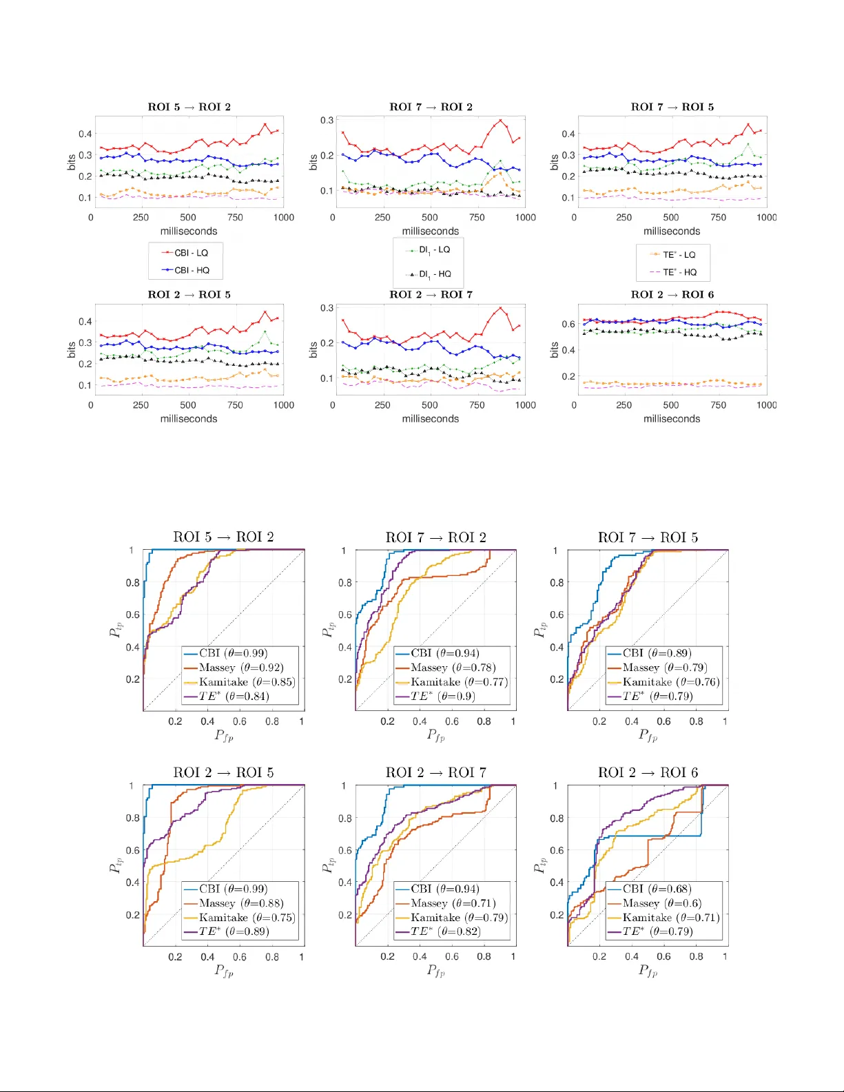
1 Directional and Causal Information Flo w in EEG for Assessing Percei v ed Audio Quality K etan Mehta ∗ and J ¨ org Klie wer † , Senior Member , IEEE ∗ Klipsch School of Electrical and Computer Engineering, Ne w Mexico State Uni versity , NM 88003 † Helen and John C. Hartmann Dept. of Electrical and Computer Engineering, Ne w Jersey Institute of T echnology , NJ 07103 Abstract —In this paper , electroencephalography (EEG) mea- surements are used to infer change in cortical functional con- nectivity in response to change in audio stimulus. Experiments are conducted wherein the EEG activity of human subjects is recorded as they listen to audio sequences whose quality varies with time. A causal information theor etic framework is then proposed to measure the inf ormation flow between EEG sensors appropriately grouped into different regions of inter est (R OI) over the cortex. A new causal bidirectional information (CBI) measure is defined as an improvement over standard directed information measures for the purposes of identifying connectivity between R OIs in a generalized cortical network setting. CBI can be intuitively interpreted as a causal bidirectional modification of directed inf ormation, and inherently calculates the divergence of the observed data from a multiple access channel with feedback. Further , we determine the analytical relationship between the different causal measures and compare how well they are able to distinguish between the per ceived audio quality . The connectivity results inferred indicate a significant change in the rate of information flow between ROIs as the subjects listen to different audio qualities, with CBI being the best in discriminating between the perceiv ed audio quality , compared to using standard directed information measures. Index T erms —Electroencephalograph y (EEG), dir ected inf or - mation, causal conditioning, functional connectivity , audio quality I . I N T RO D U C T I O N Detection and response to stimuli is in general a multistage process that results in the hierarchical activ ation and interac- tion of several different regions in the brain. T o understand the dynamics of brain functioning it therefore essential to in vestigate the information flow and connectivity (interactions) between different regions in the brain. Further , in each of these hierarchies, sensory and motor information in the brain is represented and manipulated in the form of neural acti vity patterns. The superposition of this electrophysiological acti vity can be recorded via electrodes on the scalp and is termed as electroencephalography (EEG). Functional connectivity refers to the statistical dependencies between neural data recorded from spatially distinct regions in the brain [3], [4]. Information theory provides a stochastic framew ork which is fundamentally well suited for the task of assessing functional connectivity [5], [6] between neural responses. For example, [7], [8] presented mutual information This work was supported in part by NSF grant CCF-1065603, and presented in part at the 49th Asilomar Conference on Signals, Systems and Computers [1], and at the 2017 IEEE International Conference on Communications [2]. (MI) [9] estimates to assess the correlation between the spike timing of an ensemble of neurons. Like wise, [10]– [12] in vestigated the ef fectiveness of calculating pairwise maximum entropy to model the activity of a lar ger population of neurons. MI has also has been successfully employed in the past for determining the functional connecti vity in EEG sensors for feature extraction and classification purposes [13], [14]. Similarly , other studies hav e used MI to analyze EEG data to in vestigate corticocortical information transmission for pathological conditions such as Alzheimer’ s disease [15] and schizophrenia [16], or for odor stimulation [17], [18]. One limitation of MI and entropy when applied in the traditional (Shannon) sense is their inability to distinguish between the direction of information flow , as pointed out by Marko in [19]. In the same work Marko also proposed to calculate the information flow in each direction of a bidirectional channel using conditional probabilities based on Markovian dependencies. In [20], Massey extended the initial work by Marko and formally defined directed information as the information flow from the input to the output of a channel with feedback. Other measures have similarly been defined for calculating the directional information transfer rate between random processes, most notably , Kamitake’ s directed information [21] and transfer entropy by Schreiber [22]. Further , feedback and directionality are also closely related to the notion of causality in information measures 1 [20], [23], [24]. Massey’ s directed information and transfer entropy are in general referred to as causal , since the y measure statistical dependencies between the past and current v alues of a process. W e adopt this definition in this paper and therefore, causality here takes on the usual meaning of a cause occurring prior to its ef fect, or a stimulus occurring before response, i.e., how the past states of a system influences its present and future states [25]. Our interest here is in using EEG for assessing human perception of time-v arying audio quality . W e are inspired by our recent results in [26] which uses MI to quantify the infor - mation flow ov er the end-to-end perceptual processing chain from audio stimulus to EEG output. One characteristic com- mon in subjectiv e audio testing protocols including the current state-of-the-art approach, Multi Stimulus with Hidden Anchor 1 Causality and directionality are formally defined in Def. 1 and Def. 2, resp., in Sec. III. 2 (MUSHRA) [27], is that they require human participants to assign a single quality-rating score to each test sequence. Such con ventional testing suf fers from a subject-based bias tow ards cultural factors in the local testing en vironment and can tend to be highly variable. Instead, neurophysiological measurements such as EEG directly capture and analyze the brainw av e response patterns that depend only on the percei ved variation in signal quality [28], [29]. As a result, EEG is inherently well suited to assess human perception of audio [30], [31] and visual [31]–[33] quality . F or e xample, in [31], [32] the authors used linear discriminant analysis classifiers to extract features from EEG for classifying noise detection in audio signals and to assess changes in perceptual video quality , respectiv ely . Similarly , [30] identified features in EEG brainwa ve responses corresponding to time-varying audio quality using a time- space-frequency analysis, while [33] employed a wav elet- based approach for an EEG classification of commonly occur- ring artifacts in compressed video, using a single-trial EEG. T o the best of our kno wledge, ho wev er , the work presented here is the first time that functional connectivity has been applied in conjunction with EEG measurements for the pur- poses of assessing audio quality perception. By using causal information measures to detect a change in functional con- nectivity we directly identify those cortical regions which are most actively in volved in perceiving a change in audio quality. Further , we establish the analytical relationship between the different presented information measures and compare how well each of them is able to distinguish between the percei ved audio qualities. T o wards this end, we consider two distinct scenarios for estimating the connectivity between EEG sensors by appropriately grouping them into regions of interest (R OIs) ov er the cortex. In the first scenario, we employ Massey’ s and Kamitake’ s directed information and transfer entropy , respec- tiv ely , to calculate the pairwise directional information flow between R OIs while using causal conditioning to account for the influence from all other regions. In the second scenario we propose a novel information measure which can be considered as a causal bidirectional modification of directed information applied to a generalized cortical network setting. In particular, we sho w that the proposed causal bidirectional information (CBI) measure assesses the direct connectivity between any two giv en nodes of a multiterminal cortical network by in- herently calculating the di ver gence of the induced conditional distributions from those associated with a multiple access channel (MA C) with feedback. Each presented measure is validated by applying it to analyze real EEG data recorded for human subjects as they listen to audio sequences whose quality changes over time. For the sake of simplicity and analytical tractability we restrict ourselves to only two levels of audio quality (high quality and degraded quality). W e determine and compare the instantaneous information transfer rates as inferred by each of these measures for the case where the subject listens to high quality audio as opposed to the case when the subject listens to degraded quality audio. Finally , note that we are not able make any assumptions about the actual structure of the underlying cortical channels (e.g., linear vs. non-linear) as our analysis is solely based on the observed empirical distributions of the data at the input and output of these channels. The rest of the paper is organized as follows. Section II provides an o vervie w of EEG, the experiment, and the stimulus audio sequences. In Section III we revie w some directional in- formation measures widely used in the literature for estimating connectivity . W e assess the information flow between cortical regions using directional information measures in Section IV , along with determining the analytical relationship between these measures. In Section V we introduce CBI and discuss its properties. The results of our analysis on EEG data are presented in Section VI. W e finally conclude with a summary of our study and future directions in Section VII. I I . B A C K G RO U N D In the conducted study , the EEG response activity of human test subjects is recorded as they listen to a v ariety of audio test-sequences. The quality of these stimulus test-sequences is varied with time between different “quality lev els”. All audio test-sequences were created from three fundamentally different base-sequences sampled at a reference base quality of 44.1 kHz, with a precision of 16 bits per sample. Here, we employ the same test-sequences and distortion quality lev els as in [34]. T wo different types of distortions are con- sidered for our analysis, scalar quantization and frequency band truncation, where the specific parameters are listed in T able 1. The test-sequence for a specific trial is created by selecting one of the two distortion types and then applying it to the original base-sequence in a time-varying pattern of non- ov erlapping five second blocks as shown in Fig. 1. Multiple of such trials are conducted for each subject by choosing all possible combinations of sequences, distortion types, and time- varying patterns. Note that despite the subjects being presented with all different quality le vels in our listening tests, here we focus e xemplary only on the “high” base-quality and the “Q3 degraded” quality audio. This addresses the worst-case quality change and keeps the problem analytically and numerically tractable. A detailed exposition of the experimental setup, test- sequences, and distortion quality le vels is provided in [26]. Fig. 1: A 30 second test sequence where the audio quality changes in a time-varying pattern over the whole duration of the sequence. Different possible combinations of quality changes and two distortion types are presented to each subject in a randomized fashion (adopted from [26]). T ABLE I: Different quality lev els presented to the subject during the course of an audio trial. T o generate the distortion, each of these base- sequences were passed through a 2048-point modified discrete cosine transform and either frequenc y truncation or scalar quantization was applied to the coefficients prior to reconstruction [34]. Quality Level Freq. Truncation Scalar Quantization Low Pass Filter No. of Significant Bits Retained Q1 4.4 KHz 4 Q2 2.2 KHz 3 Q3 1.1 KHz 2 3 Fig. 2: The 128 electrodes are grouped into eight regions of interest (R OI) to ef fectiv ely cover the dif ferent cortical regions (lobes) of the brain (adopted from [26]). The red electrode locations are used for generating synthetic EEG data in Sec. VI-C, see T able III for the naming conv ention. The EEG data is captured on a total of 128 spatial channels using an Activ eT wo Biosemi system with a sampling rate of 256 Hz. T o better manage the large amount of collected data while also effecti vely cov ering the activity over different regions of the cortex, we group the 128 electrodes into specific regions of interest (R OI) as shown in Fig. 2. While a large number of potential grouping schemes are possible, this scheme is fav ored for our purposes as it efficiently cov ers all the cortical regions (lobes) of the brain with a relativ ely low number of ROIs. Also, the number of electrodes in any giv en R OI varies between a minimum of 9 to a maximum of 12. For example, in our re gion partitioning scheme R OI 2 (9 electrodes) covers the prefrontal cortex, ROI 6 (10 electrodes) the parietal lobe, R OI 8 (9 electrodes) the occipital lobe, and R OI 5 and R OI 7 (12 electrodes each) cov er the left and right temporal lobes, respectiv ely . In essence, our goal here then is to in vestigate the causal connecti vity between the different R OI in response to the different audio quality levels. I I I . D I R E C T I O NA L I T Y , C AU S A L I T Y A N D F E E D BA C K I N I N F O R M A T I O N M E A S U R E S Let X n denote a random vector of n constituent discrete valued random variables [ X 1 , X 2 , . . . , X n ] . Also, let x n = [ x 1 , x 2 , . . . , x n ] be the corresponding realizations drawn from the joint probability distrib ution denoted by p ( x 1 , x 2 , . . . , x n ) , respectiv ely . Similarly , X N n = [ X n , X n +1 , · · · , X N ] repre- sents a length N − n + 1 random vector . Denoting the expected value of a random variable by E [ · ] , the entropy of the n -tuple X n can be written as H ( X n ) = − E [log p ( X n )] . The mutual information (MI) between two length N inter- acting random processes X N and Y N is defined as I ( X N ; Y N ) = N X n =1 I ( X N ; Y n | Y n − 1 ) (1) = H ( Y N ) − H ( Y N | X N ) , (2) with the conditional entropy H ( Y n | X n ) = − E [log p ( Y n | X n )] and H ( Y N | X N ) = N X n =1 H ( Y n | Y n − 1 X N ) . (3) The MI measures the reduction in the uncertainty of Y N due to the knowledge of X N , and is zero if and only if the two processes are statistically independent. The MI between the two random processes is symmetric, i.e., I ( X N ; Y N ) = I ( Y N ; X N ) , and can therefore not distinguish between the direction of the information flow . Alternatively , a directional information measure introduces the notion of direction in the exchange of information between sources. In this paper we define a directional information measure as follo ws. Definition 1. A dir ectional information measur e fr om X N to Y N , repr esented with an arrow X N → Y N , quantifies the information e xchang e rate in the direction fr om the input pr ocess X N towar ds the output pr ocess Y N . As implied by the definition, the information flow measured by a directional information measure is not symmetric, and in general the flow from X N → Y N is not equal to Y N → X N . In the following, we will examine three different directional information measures presented in the literature. A. Masse y’ s dir ected information Directed information as proposed by Massey in [20] is an e xtension of the preliminary w ork by Marko [19] to characterize the information flow on a communication channel with feedback. Giv en input X N and output Y N , the channel is said to be used without feedback if p ( x n | y n − 1 x n − 1 ) = p ( x n | x n − 1 ) , ∀ n ≤ N , (4) i.e., the current channel input value does not depend on the past output samples. If the channel is used with feedback then [20] shows that the chain rule of conditional probability can be reduced to p ( y N | x N ) = N Y n =1 p ( y n | y n − 1 x n ) . (5) In closely related work [35] introduced the concept of causal conditioning based on (5). The entropy of Y N causally conditioned on X N is defined as H ( Y N || X N ) = N X n =1 H ( Y n | Y n − 1 X n ) . (6) Definition 2. A measure between two random processes X N and Y N is said to be causal if the information transfer rate at time n relies only on the dependencies between their past and current sample values X n and Y n , and is not a function of the future sample values X N n +1 and Y N n +1 . Therefore, the notion of causality as used in this work is based on inferring the statistical dependencies between the past states of a system on its present and future states [20], [23]–[25]. This is in contrast to the stronger interventional interpretation about casual inferences such as in [36] which 4 draws conclusions about causation , e.g., process X N causes Y N . Massey’ s directed information is a causal measure between sequence X N and Y N defined as D I 1 ( X N → Y N ) , H ( Y N ) − H ( Y N || X N ) (7) = N X n =1 I ( X n ; Y n | Y n − 1 ) . (8) Equiv alently , the directed information can also be written in terms of the Kullback-Leibler (KL) diver gence as D I 1 ( X N → Y N ) = N X n =1 D K L  p ( y n | y n − 1 x n ) || p ( y n | y n − 1 )  (9) = N X n =1 E  log p ( Y n | Y n − 1 X n ) p ( Y n | Y n − 1 )  . (10) Also in general, D I 1 ( X N → Y N ) ≤ I ( X N ; Y N ) , (11) with equality if the channel is used without feedback. Directed information therefore not only gives a meaningful notation to the directi vity of information, but also provides a tighter characterization than MI on the total information flo w over a channel with feedback. B. T ransfer entr opy In [22], Schreiber introduced a causal measure for the di- rected exchange of information between two random processes called transfer entropy . Similar to the pioneering work in [19], transfer entropy considers a bidirectional communication channel between X N and Y N , and measures the deviation of the observed distribution p ( y n | y n − 1 x n − 1 ) ov er this channel from the Markov assumption p ( y n | y n − 1 x n − 1 ) = p ( y n | y n − 1 ) , n ≤ N . (12) In particular , transfer entropy quantifies the deviation of the l.h.s. of (12) from the r .h.s. of (12) using the KL div ergence and is defined as T E ( X n − 1 → Y n ) , D K L  p ( y n | y n − 1 x n − 1 ) || p ( y n | y n − 1 )  (13) = E  log p ( Y n | Y n − 1 X n − 1 ) p ( Y n | Y n − 1 )  (14) = H ( Y n | Y n − 1 ) − H ( Y n | Y n − 1 X n − 1 ) (15) = I ( Y n ; X n − 1 | Y n − 1 ) . (16) Correspondingly , for random processes of block length N we can then define a sum transfer entropy [37], [38] which in effect calculates and adds the transfer entropy at ev ery history depth n , T E ∗ ( X N − 1 → Y N ) = N X n =1 T E ( X n − 1 → Y n ) . (17) Another widely used and closely related measure for causal influence was developed by Granger [39]. Granger causality is a directional measure of statistical dependency based on prediction via v ector auto-regression. The relationship between Granger causality and directional information measures has been previously analyzed in [40], [41]. For the specific case of Gaussian random variables, as it is the case in our EEG scenario, transfer entropy has been sho wn to be equiv alent to Granger causality . C. Kamitake’ s directed information Another v ariant of directed information is defined by Kami- take in [21] and gi ven as D I 2 ( X N → Y N ) , N X n =1 I ( X n ; Y N n +1 | X n − 1 Y n ) (18) = H ( Y N n +1 | X n − 1 Y n ) − H ( Y N n +1 | X n Y n ) . (19) W e notice that this measure is dif ferent from Massey’ s directed information in that it measures the influence of the current sample X n of X N at time n on the future samples Y N n +1 of Y N . Kamitake’ s information measure is therefore directional, but not causal. I V . A S S E S S I N G C O RT I C A L I N F O R M AT I ON F L O W V I A D I R E C T I O NA L M E A S U R E S A. Causal conditioning and indir ect influences in multitermi- nal networks A multi-terminal network characterizes the information flow between multiple communicating nodes with sev eral senders and receiv ers. Let us denote three communicating nodes X , Y , and Z and the corresponding random processes associated with them as X N , Y N , and Z N respectiv ely . In our case, the information transfer over the cortex can be considered equiv alent to a cortical multi-terminal network, with each ROI taking over the role of a communicating node. In the context of the cortical network the quantities X N , Y N , and Z N , then correspond to the sampled EEG signals from dif ferent ROIs. Also without any loss of generality , Z N represents the output of multiple (and potentially all other) ROIs. Our goal here is to identify the connectivity between the processes in the cortical network. In particular, there are two distinct instances of connectivity that can arise as a result of using directional informational measures. Definition 3. A dir ect connectivity is said to exist fr om node X to node Y if there exists a non-zer o information flow via a dir ect path between the nodes. Definition 4. An implied connectivity arises when there is no dir ect path between two nodes X and Y , but ther e is a non-zer o information flow between the nodes because of an influence thr ough other nodes in the network. Therefore, a positiv e directed information between the ran- dom processes associated with any two nodes in a multi-node network alone does not necessarily equate to a direct connec- tivity between them [41]–[43]. In Fig. 3 we show an example 5 Fig. 3: The relay channel is an example of a network in which simply using directed information can lead to a false inference of dir ect connectivity between the nodes. In the example shown, D I ( X N → Y N ) > 0 , ev en though there is no link between X and Y . network topology to illustrate how implied connectivity can lead to false inferences. In the shown relay channel there is no direct information transfer between X and Y , but the information flow is from X to Z to Y . There is a Markovian influence X → Z → Y . This results in a positive value for Massey’ s directed information, D I 1 ( X N → Y N ) > 0 , thereby leading to implied connectivity between X and Y . Notice howe ver that in the example presented, the knowl- edge of Z N leads to statistical conditional independence between X N and Y N . W e expand upon this idea and extend the expression for Massey’ s directed information to account for the influence of the additional random processes in the network via causal conditioning [35]. Definition 5. Causally conditioned Massey’ s dir ected infor- mation is defined as the information flowing from X N to Y N causally conditioned on the sequence Z N − 1 as D I 1 ( X N → Y N || Z N − 1 ) , H ( Y N || Z N − 1 ) − H ( Y N || X N Z N − 1 ) (20) = N X n =1 D K L  p ( y n | x n y n − 1 z n − 1 ) || p ( y n | y n − 1 z n − 1 )  (21) = N X n =1 I ( X n ; Y n | Y n − 1 Z n − 1 ) . (22) Proposition 1 ( [41], [42]) . Assume a network as shown in F ig. 3 with three nodes X , Y , and Z , with corresponding random processes X N , Y N , and Z N , r espectively . Using causally conditioned Massey’ s dir ected information eliminates implied connectivity , with D I 1 ( X N → Y N || Z N − 1 ) = 0 if X and Y ar e not directly connected. Both transfer entropy and Kamitake’ s directed information can be extended to incorporate causal conditioning from an additional random process as well. Definition 6 ( [44]–[46]) . Causally conditioned transfer en- tr opy and sum transfer entr opy ar e defined r espectively as T E ( X n − 1 → Y n || Z n − 1 ) , D K L  p ( y n | y n − 1 x n − 1 z n − 1 ) || p ( y n | y n − 1 z n − 1 )  (23) = I ( Y n ; X n − 1 | Y n − 1 Z n − 1 ) , (24) T E ∗ ( X N − 1 → Y N || Z N − 1 ) (a) (b) (c) Fig. 4: (a) An example of a multiterminal network with information flow existing between several nodes, for which we estimate the underlying causal connectivity . The solid arro ws denote the direction of the forw ard information flo w , while the dashed arro ws represent feedback flow between the nodes. (b), (c) Pairwise conditional directed information calculated by choosing an input and output node, while using causal conditioning to account for the influence of all other nodes. , N X n =1 T E ( X n − 1 → Y n || Z n − 1 ) . (25) Definition 7. Causally conditioned Kamitake’ s directed infor - mation is defined as D I 2 ( X N → Y N || Z N − 1 ) , N X n =1 I ( X n ; Y N n +1 | X n − 1 Y n Z n − 1 ) . (26) Similar to Massey’ s directed information, causally condi- tioned transfer entropy and Kamitake’ s directed information can also be used to eliminate false inferences resulting from implied connectivity [46], [47]. The proof follo ws along the exact same lines as Proposition 1 and is omitted here. Also, note that despite the conditioning on a causal sequence Z n − 1 , Kamitake’ s directed information measure is not strictly causal due to the Y N n +1 term. Now we discuss how to apply causally conditioned direc- tional information measures in order to estimate the functional connectivity between the R OI netw ork. In Fig. 4(a) we show an example communication network with four interacting nodes. The information flow is depicted using solid arrows and the feedback using dashed arrows, respectiv ely . Also, some nodes do not ha ve a direct link in between them, for example X to A . In our cortical network model the nodes represent the R OIs, and the quantities X N , Y N , A N and B N , resp., represent the random processes describing the sampled output of the EEG signals in each R OI. Our goal is then to infer the causal connectivity between the R OIs given the EEG recordings from each region. T ow ards this end we propose calculating the pairwise conditional directed information by choosing 6 an input and output node, while using causal conditioning to account for the influence of all other nodes. For exam- ple, to estimate the connectivity from X to Y we calculate D I 1 ( X N → Y N || A N B N ) as shown in Fig. 4(b). Since there is non-zero information flow between these two nodes we expect the directed information to return a positive v alue. Similarly in Fig. 4(c), computing D I 1 ( X N → A N || Y N B N ) yields a zero value since there is no direct connectivity between these two nodes. Repeating this procedure pairwise for all nodes provides a functional connectivity graph representativ e of the directional information flow over the entire ROI network. B. Relationship between differ ent measur es The first relation that we are interested in is between Massey’ s and Kamitake’ s directed information measures as examined in [48], [49]. W e extend this analysis to include causal conditioning on Z N − 1 and show its connection to causally conditioned MI. Proposition 2. The r elation between causally conditioned Masse y’ s and causally conditioned Kamitake’ s dir ected infor- mation is given by D I 2 ( Y N → X N || Z N − 1 ) + D I 1 ( X N → Y N || Z N − 1 ) = D I 2 ( X N → Y N || Z N − 1 )+ D I 1 ( Y N → X N || Z N − 1 ) . (27) Pr oof. Using the definition in (26) and rewriting in terms of entropy D I 2 ( Y N → X N || Z N − 1 ) = N X n =1 I ( Y n ; X N n +1 | X n Y n − 1 Z n − 1 ) (28) = N X n =1  H ( X N n +1 | X n Y n − 1 Z n − 1 ) − H ( X N n +1 | X n Y n Z n − 1 )  (29) = N X n =1  H ( X N | Y n − 1 Z n − 1 ) − H ( X n | Y n − 1 Z n − 1 ) − H ( X N | Y n Z n − 1 ) + H ( X n | Y n Z n − 1 )  (30) = N X n =1 I ( X N ; Y n | Y n − 1 Z n − 1 ) − D I 1 ( X N → Y N || Z N − 1 ) , (31) where we hav e used the chain rule of entropy in (30). Rearranging yields D I 2 ( Y N → X N || Z N − 1 ) + D I 1 ( X N → Y N || Z N − 1 ) = N X n =1 I ( X N ; Y n | Y n − 1 Z n − 1 ) (32) = N X n =1 N X i =1 I ( X i ; Y n | X i − 1 Y n − 1 Z n − 1 ) (33) = N X n =1 I ( Y N ; X n | X n − 1 Z n − 1 ) (34) = D I 2 ( X N → Y N || Z N − 1 ) + D I 1 ( Y N → X N || Z N − 1 ) , (35) where (33) follows by using the chain rule of MI, and (34) from interchanging the order of summation. Definition 8. Causally conditioned MI is defined as the MI between X N and Y N causally conditioned on the sequence Z N − 1 I ( X N ; Y N || Z N − 1 ) , N X n =1 I ( X N ; Y n | Y n − 1 Z n − 1 ) = N X n =1 I ( X n ; Y N | X n − 1 Z n − 1 ) . (36) The following corollary then expresses causally conditioned MI in terms of directed information and follows directly from (32)-(34) in the proof of Proposition 2. Corollary 3. Causally conditioned MI is the sum of causally conditioned Massey’ s dir ected information from X N to Y N , and causally conditioned Kamitake’ s dir ected information in the opposite direction: I ( X N ; Y N || Z N − 1 ) = D I 1 ( X N → Y N || Z N − 1 ) + D I 2 ( Y N → X N || Z N − 1 ) . (37) There also exists a connection between between Massey’ s directed information and transfer entropy as shown in [38], [50], [51], which we extend and state for causal conditioning as follows. Proposition 4. The r elation between causally conditioned Masse y’ s dir ected information and causally conditioned tr ans- fer entr opy is given by D I 1 ( X N → Y N || Z N − 1 ) = N X n =1  T E ( X n − 1 → Y n || Z n − 1 ) + I ( X n ; Y n | X n − 1 Y n − 1 Z n − 1 )  . (38) W e observe that the directed information is a sum over the transfer entropy and an additional term describing the conditional undirected MI between X n and Y n . Massey’ s directed information as defined in Sec. III-A was originally intended to measure the dependency between two N length sequences. If we now relax this constraint to instead suitably measure the flow from a N − 1 length sequence X N − 1 to a N length sequence Y N , while causally conditioned on Z N − 1 , we then ha ve a modified interpretation for causally conditioned Massey’ s directed information which we denote as D I 0 1 and define as follows, D I 0 1 ( X N − 1 → Y N || Z N − 1 ) = T E ∗ ( X N − 1 → Y N || Z N − 1 ) (39) where the equality in (39) follows directly from from (24). Further , if we assume the sequences to be stationary and infinitely long and that the limit for N → ∞ exists, then asymptotically it can be shown [38], [51] that the information rates for causally conditioned Massey’ s modified directed information D I 0 1 and causally conditioned transfer entropy (23) are in fact equal. 7 V . C AU S A L B I D I R E C T I O N A L I N F O R M A T I O N F L O W I N E E G In the follo wing we propose an alternati ve bidirectional measure for estimating the causal dependency between the R OIs. This measure is motiv ated by the analysis of the three- terminal multiple access channel (MAC) with feedback, an important canonical building structure in networked commu- nication. A. Causal bidir ectional information (CBI) In order to derive the CBI measure let us first consider a preliminary result which uses causally conditioned directed information to express the information rate for such a MA C with feedback. Fig. 5 shows a two user MA C with feedback, with channel inputs X and Y , and corresponding output Z . The capacity region for the two user discrete memoryless MA C with feedback can be lower bounded using directed information, in a form similar to the standard cut-set bound for the MA C without feedback [9]. The information rate from X N to Z N is shown to be [35], R 1 ≤ 1 N D I ( X N → Z N || Y N ) for all p ( x n y n | x n − 1 y n − 1 z n − 1 ) = p ( x n | x n − 1 z n − 1 ) · p ( y n | y n − 1 z n − 1 ) , n ≤ N . (40) The other rate R 2 from Y to Z and the sum rate R 1 + R 2 can be found in [35] and are not of interest for the following discussion. Fig. 5: A multiple access channel with feedback. Now , consider the scenario of a general multi-terminal network as shown in Fig. 6(a), where each node sends in- formation and receives feedback from ev ery other node in the network. CBI considers the three node network of Fig. 6(a) and measures the information flow in between nodes X and Y by using the MA C as a reference, as shown in Fig. 6(b). In particular , we point our attention tow ards the relation in (40) specifying the relation between the joint distribution of the two inputs of the MAC. The conditional independence of the inputs in the factorization of (40) arises due to the causal nature of the feedback structure, where the output at the receiv er Z n − 1 is av ailable causally at both X and Y for each time n . For the case of a MAC with feedback there is no direct connectivity (path) between the inputs. Any violation of (40) creates dependencies between X and Y , and these dependencies can be measured by the KL div ergence between the joint distribution on the l.h.s. of (40) and the factorization on the r .h.s. of (40). This result is summarized in the follo wing definition. (a) (b) Fig. 6: (a) A general multi-terminal network whose connectivity we are interested in. All three communicating nodes send and receiv e information from each other . (b) CBI infers the connectivity between X and Y by calculating the diver gence of the observed joint distribution on the network of Fig. 6(a) from the one of a MAC with feedback in (40). Definition 9. Consider a multi-terminal network with a sour ce node X , a destination node Y , and a gr oup of nodes Z inter- acting casually with X and Y as shown in F ig. 6(a). CBI cal- culates the KL diver gence between the induced distributions of the observed conditional distribution p ( x n y n | x n − 1 y n − 1 z n − 1 ) and the one for an underlying MA C with feedback (40): I ( X N  Y N || Z N − 1 ) = D K L  p ( x n y n | x n − 1 y n − 1 z n − 1 ) || p ( x n | x n − 1 z n − 1 ) p ( y n | y n − 1 z n − 1 )  (41) = N X n =1 E  log p ( X n Y n | X n − 1 Y n − 1 Z n − 1 ) p ( X n | X n − 1 Z n − 1 ) p ( Y n | Y n − 1 Z n − 1 )  (42) = H ( X N || Z N − 1 ) + H ( Y N || Z N − 1 ) − H ( X N Y N || Z N − 1 ) . (43) Therefore, CBI ascertains the direct connectivity (as per Def. 3) between two nodes in a general multi-node network and is zero if and only if the following two conditions are satisfied: (i) X n and Y n are independent for all n ≤ N , i.e., there is no information flow between the two nodes. (ii) There is no direct link between X and Y and all infor- mation flows only via an additional node Z . In the following proposition we sho w that, by defini- tion, CBI is inherently a casual bidirectional modification of Massey’ s directed information. Proposition 5. Causal bidirectional information (CBI) is the sum of causally conditioned Massey’ s directed information between X N and Y N , and the sum transfer entr opy in the r everse dir ection: 8 I ( X N  Y N || Z N − 1 ) , D I 1 ( X N → Y N || Z N − 1 ) + N X n =1 n T E ( Y n → X n || Z n − 1 ) o . (44) Pr oof. W e start with D I 1 ( X N → Y N || Z N − 1 ) + T E ∗ ( Y N − 1 → X N || Z N − 1 ) = N X n =1 n I ( Y n ; X n | Y n − 1 Z n − 1 ) + T E ( Y n − 1 → X n || Z n − 1 ) o , (45) where the equality in (45) follows from (22) in Definition 5. Denoting the term inside the summation on the r .h.s. of (45) by Φ( · ) and rewriting yields Φ( x n , y n , z n − 1 ) = I ( Y n ; X n | Y n − 1 Z n − 1 ) + T E ( Y n − 1 → X n || Z n − 1 ) (46) = E  log p ( Y n | X n Y n − 1 Z n − 1 ) p ( Y n | Y n − 1 Z n − 1 )  + E  log p ( X n | Y n − 1 X n − 1 Z n − 1 ) p ( X n | X n − 1 Z n − 1 )  (47) = E  log p ( Y n X n | Y n − 1 X n − 1 Z n − 1 ) p ( Y n | Y n − 1 Z n − 1 ) p ( X n | X n − 1 Z n − 1 )  , (48) where in (47) we ha ve made use of (21) and (23), respecti vely , and (48) follows from the chain rule of joint probability p ( y n x n | x n − 1 y n − 1 z n − 1 ) = p ( y n | x n x n − 1 y n − 1 z n − 1 ) · p ( x n | x n − 1 y n − 1 z n − 1 ) . (49) T aking the summation on (48) and comparing with (42) prov es the claim. Corollary 6. CBI is a symmetric measur e I ( X N  Y N || Z N − 1 ) = D I 1 ( X N → Y N || Z N − 1 ) + T E ∗ ( Y N − 1 → X N || Z N − 1 ) (50) = D I 1 ( Y N → X N || Z N − 1 ) + T E ∗ ( X N − 1 → Y N || Z N − 1 ) . (51) Pr oof. Without any loss of generality , the joint probability distribution in (49) can alternatively be expanded as p ( y n x n | y n − 1 x n − 1 z n − 1 ) = p ( x n | y n y n − 1 x n − 1 z n − 1 ) · p ( y n | y n − 1 x n − 1 z n − 1 ) . (52) Using the above equation and rewriting (48) then gives us Φ( x n , y n , z n − 1 ) = E  log p ( Y n X n | Y n − 1 X n − 1 Z n − 1 ) p ( Y n | Y n − 1 Z n − 1 ) p ( X n | X n − 1 Z n − 1 )  (53) = E  log p ( X n | Y n X n − 1 Z n − 1 ) p ( X n | X n − 1 Z n − 1 )  + E  log p ( Y n | Y n − 1 X n − 1 Z n − 1 ) p ( Y n | Y n − 1 Z n − 1 )  (54) = I ( X n ; Y n | X n − 1 Z n − 1 ) + T E ( X n − 1 → Y n || Z n − 1 ) . (55) T aking the sum on both sides of (55) yields the required result. W e also ev aluate the expression for CBI by comparing it to conditional MI. Conditional MI measures the diver gence between the actual observ ations and those which would be ob- served under the Markovian assumption X N ↔ Z N − 1 ↔ Y N , I ( X N ; Y N | Z N − 1 ) = E  log p ( X N Y N | Z N − 1 ) p ( X N | Z N − 1 ) p ( Y N | Z N − 1 )  (56) = N X n =1 E  log p ( X n Y n | X n − 1 Y n − 1 Z N − 1 ) p ( X n | X n − 1 Z N − 1 ) p ( Y n | Y n − 1 Z N − 1 )  (57) = H ( X N | Z N − 1 ) + H ( Y N | Z N − 1 ) − H ( X N Y N | Z N − 1 ) , (58) where (57) follows from the chain rule of probability . Condi- tional MI is zero if and only if X N and Y N are conditionally independent gi ven Z N − 1 . By comparing conditional mutual information (57) with the expression for CBI in (42), we notice that CBI uses causal conditioning as Z N − 1 is replaced with Z n − 1 . V I . I N F E R R I N G C H A N G E I N F U N C T I O N A L C O N N E C T I V I T Y A. Pr eliminaries In our analysis, we separately extract the EEG response sections for each of the two audio quality levels and calculate the information measures individually for each of them. This allows us to compare how the different probability distribu- tions used in each of the presented information measures ef fect the ability to detect a change in information flo w among the R OIs in Fig. 2, between the cases when the subjects listen to high quality audio as opposed to de graded quality audio. W e begin by selecting a source and a destination R OI, X and Y , respectively . The other six remaining R OIs are considered to represent the side information Z . Since all electrodes in a ROI are located within close proximity of one another and capture data ov er the same cortical region, we consider ev ery electrode in an R OI as an independent realization of the same random process. For example, the sampled EEG data recorded on ev ery electrode within region X , in a giv en time interval N , is considered a realization of the same random process X N . This increases the sample size for the process X N , reducing the expected deviation between the obtained empirical distribution of X N and the true one. The discussed information measures are therefore calculated between the R OI pairs (and not between individual electrodes) for a total of 2-permutations of 8 R OIs, i.e., 56 combinations of source- destination pairs. In our earlier work [26] we demonstrated that the output EEG response to the audio quality , ov er an ROI, con ver ges to a Gaussian distrib ution with zero mean. The intuition here is that the potential recorded at the EEG electrode at any gi ven time- instant can be considered as the superposition of responses of a large number of neurons. Thus, the distribution of a suf ficiently 9 high number of these trials taken at different time instances con verges to a Gaussian distribution as a result of the Central Limit Theorem. Fig. 7 shows the histogram of the sampled EEG data, formed by concatenating the output over all sensors in one R OI for a single subject. The sample ske wness and kurtosis of the EEG output distribution are shown in T able II. For a Gaussian distribution the skewness equals 0 and the kurtosis equals 3 [52], [53]. T o test Gaussanity of a large sample set, the sample ske wness and kurtosis should approach these values, while an absolute skew value larger than 2 [53] or kurtosis larger than 7 [54] may be used as reference values for determining substantial non-normality . By inspecting the sample estimates in T able II and comparing the histogram to a Gaussian distribution in Fig. 7, we observe that the EEG output distribution is indeed strongly Gaussian. Knowing that the interacting random processes from the R OIs con verge to a Gaussian distribution [26] allows us to for- mulate analytical closed-form expressions for calculating the information measures. The joint entropy of a n -dimensional multiv ariate Gaussian distrib ution with probability density p ( z 1 . . . z n ) is known to be given by [9] H ( Z 1 . . . Z n ) = 1 2 log (2 π e ) n | C ( Z 1 . . . Z n ) | , (59) where C ( · ) is the cov ariance matrix and | · | is the determinant of the matrix. If X N , Y N , and Z N are jointly Gaussian distributed, then using (59) in conjunction with (43) reduces CBI to a function of their joint covariance matrices, I ( X N  Y N || Z N − 1 ) = 1 2 N X n =1 log ( | C ( X n − 1 Y n − 1 Z n − 1 ) | | C ( X n Y n Z n − 1 ) | · | C ( X n Z n − 1 ) | · | C ( Y n Z n − 1 ) | | C ( X n − 1 Z n − 1 ) | · | C ( Y n − 1 Z n − 1 ) | ) . (60) In a similar manner , causally conditioned Massey’ s directed information, Kamitake’ s directed information, and sum trans- fer entropy , resp., can be reduced to obtain the following expressions, D I 1 ( X N → Y N || Z N − 1 ) = 1 2 N X n =1 log | C ( Y n Z n − 1 ) | · | C ( X n Y n − 1 Z n − 1 ) | | C ( Y n − 1 Z n − 1 ) | · | C ( X n Y n Z n − 1 ) | , (61) D I 2 ( X N → Y N || Z N − 1 ) = 1 2 N X n =1 log | C ( X n − 1 Y N Z n − 1 ) | · | C ( X n Y n Z n − 1 ) | | C ( X n − 1 Y n Z n − 1 ) | · | C ( X n Y N Z n − 1 ) | , (62) T E ∗ ( X N − 1 → Y N || Z N − 1 ) = 1 2 N X n =1 log | C ( Y n Z n − 1 ) | · | C ( Y n − 1 X n − 1 Z n − 1 ) | | C ( Y n − 1 Z n − 1 ) | · | C ( Y n X n − 1 Z n − 1 ) | . (63) B. Receiver operating char acteristic (R OC) curves In order to ev aluate the accuracy with which an informa- tion measure and in particular CBI can distinguish between Fig. 7: Sampled EEG output distributions over a single ROI for high quality and frequency distorted audio input-stimulus, respectiv ely . The data used to construct the histogram is the combined output ov er all sensors in R OI 5 during the period of a single frequency- truncated trial, for Subject S1. The Gaussian fit is obtained by using an estimator that minimizes the L 1 distance between the fitted Gaussian distribution and the histogram data. T ABLE II: Sample skewness and kurtosis estimated for a single subject S1 using data from a single frequency-truncated trial. The sampled EEG data for a given R OI was obtained by concatenating the output of all electrodes in that ROI. HQ LQ R OI Mean Ske w- ness Kurto- sis Mean Ske w- ness Kurto- sis 1 -0.003 0.180 2.820 -0.014 0.187 2.816 2 0.148 0.057 2.943 0.159 0.214 2.786 3 0.027 0.069 2.931 0.014 0.054 2.945 4 0.216 -0.154 3.155 0.2975 0.131 2.869 5 -0.058 -0.132 3.133 -0.073 -0.103 3.103 6 -0.305 -0.145 3.146 -0.283 -0.259 3.260 7 -0.111 0.016 2.984 -0.101 0.050 2.950 8 0.465 -0.070 3.071 0.445 -0.342 3.342 the perceiv ed audio quality we conduct a receiver operating characteristic (R OC) curve analysis [55], [56] on the generated vectors of measurements for the high and degraded quality audio, respectiv ely . The ROC curve serves as a non-parametric statistical test to compare dif ferent information rates [57]–[60] and has the advantage that a test statistics can be generated from the observed measurements. Consider a general binary classification scheme between two classes P and N , labeled as positive and ne gative , respectiv ely . These classes contain samples from the respecti ve class distributions with |P | = N p and |N | = N n . Also, ev ery individual instance from the positiv e class is associated with a known measurement score S ( p ) i which is a random vari- able with an unknown distribution and corresponding values s ( p ) i , i = 1 , . . . , N p . Similarly , for the negati ve class we have the random variable S ( n ) i with values s ( n ) i , i = 1 , . . . , N n . For a given discrimination threshold value T , the classi- fication rule is such that the individual is allocated to the 10 positiv e class if its score exceeds the threshold, i.e., s ( p ) i > T . Else, s ( p ) i ≤ T , then the instance is allocated to the negati ve class. The true positiv e probability [56] is the probability that an individual from the positi ve class is correctly classified as belonging to the positive class: P tp ( T ) = P N p i =1 1 ( s ( p ) i > T ) N p , (64) where 1 ( · ) denotes the indicator function. Like wise, the false positiv e probability is the probability that an individual from the negati ve population is misclassified (incorrectly allocated) as belonging to the positi ve population: P f p ( T ) = P N n i =1 1 ( s ( n ) i > T ) N n . (65) Since in general the best choice for T is not known, the measurement scores themselves often serv e as optimal choices for the discrimination threshold values [55]. The R OC curve is then a graphical representation obtained by plotting the true positiv e probability P tp ( T ) versus the false positiv e probability P f p ( T ) as a function of the discrimination threshold value T . The area under the R OC curve, denoted using the v ariable θ , summarizes the results over all possible values of the threshold T [55], [61], with possible values ranging from θ = 0 . 5 (no discriminativ e ability) to θ = 1 . 0 (perfect discriminativ e ability). In fact, the area under the curve is shown to be equivalent to the Wilcoxon-Mann-Whitne y non- parametric test-statistic [52] and can be used to determine whether samples selected from the two class populations have the same distribution [62], [63]. More specifically , the area under the ROC curve is equiv alent to the probability that a randomly selected instance from the positiv e class will have a measurement score that is greater than a randomly selected instance from the negativ e class. C. P erformance of information measur es on simulated EEG data T o obtain an initial assessment of the information measures introduced in Sec. IV and Sec. V , we apply these measures to synthetic EEG data. The advantage of this approach is that the true causal connectivity graph of the simulated network is known and that, in contrast to real EEG data obtained from human subjects, in principle there is no limitation to the number of trials. The EEG data is created using a wav elet transform following the approach described in [64], wherein the EEG is decomposed as a con volution of a series of basis functions (i.e., wavelets) within selected frequenc y bands listed in T able III. In [64] the probability distribution of the wavelet coefficients for each frequency band was estimated using real human EEG data sampled at 250Hz, which was shown to be a logistic distribution with heavier tails than a Gaussian distribution. W e now generate simulated wav elet coefficients for a particular frequency band by multiplying the associated logistic distribution with a constant scaling factor and then randomly dra wing samples from this scaled distribution. The simulated EEG signal is then obtained by an in verse wav elet transform of these randomly drawn samples for all frequency bands in T able III. In this work, two dif ferent sets of scaling T ABLE III: W avelet coef ficient scale factor for high and low acti vity for each source-sink pair . Source Sink Freq. (Hz) High Low Fz Cz 0 - 3.91 (delta) U (0.9, 1) U (0.55, 0.85) F5, F6 P5, P6 3.91 - 7.81 (theta) U (0.9, 1) U (0.55, 0.85) P6, F5 Cz 7.81 - 15.62 (alpha) 1 1 T7 T8 15.62 - 31.25 (beta) 1 1 factors are used to simulate change in network connectivity . Since the magnitude of the scaling coefficient controls the spectral energy (activity) in that band, we here use the activity labels “high” and “low”, respectiv ely , to differentiate between these two sets of connectivities as shown in T able III. For simulation purposes, the wavelet-coef ficients for high activity in the delta band (0-3.91 Hz) and theta band (3.91-7.81 Hz) are scaled by a factor chosen from a distribution U (0 . 9 , 1) , where U ( a, b ) denotes the uniform distribution within the interval ( a, b ) . Low acti vity is simulated by choosing the scaling factors for the delta and theta bands from U (0 . 55 , 0 . 85) . Note that the uniform distribution and the associated intervals are only chosen to demonstrate a change in delta and theta acti vity lev els, and in theory any suitable set of high-valued and low- valued scaling factors can potentially be used to this ef fect. A source and sink electrode location was assigned to each frequency band [64] as shown in T able III. The locations of these electrodes are marked in red in Fig. 2. Simulated EEG signals are generated across the scalp by spherical spline interpolation across neighboring electrodes by using the ee g interp function in EEGLAB [65]. In essence this function simulates EEG scalp topography by smearing electric potentials through volume conduction [66]. This results in a synthetic EEG wav eform at each electrode with energy within each of the four characteristic frequency bands. W e generate 1000 trials of simulated EEG data for each of the two cases of high and low activity . For each trial, a total of 430500 samples (at 250 Hz) are generated for each of the electrodes listed in T able III. The EEG output generated at each of these electrodes is tested for Gaussianity similar to the process described in Sec.VI-A, including using an estimator that minimizes the L 1 distance between the fitted Gaussian distribution and the generated data, and indeed verified to be near Gaussian. For each trial of high and low activity the source electrode (of a given frequency band for which the acti vity changed) is designated as X , the corresponding destination electrode as Y , and all other remaining electrodes in T able III are grouped together as Z . The sample space for each trial is obtained by dividing the 430500 samples into 14350 sections each of block length N = 30 (120 ms). W e then compute the dif ferent information measures (60)- (63) o ver the block length N and compare ho w the different probability distributions used in each measure effect the ability to detect change in connectivity . The corresponding cov ariance matrices, ∀ n = 1 , . . . , N , are estimated from the 14350 11 sections, assuming stationarity of the EEG signals within each section. While here we always sum up to a depth of N = 30 , we note that the estimate accuracy of the information measures, the computational time and complexity , and the probability of a false negati ve can all be further impro ved by rigorously selecting optimal history lengths [38], [67]. The ROC curv e analysis is used to test the accuracy with which these information measures can distinguish between the cases of high and low activity . The positiv e class P is constructed by concatenating the information rates for the high activity , and like wise the ne gative class N for low activity . The ROC curv e for the information measure is then constructed using the empirical probabilities P tp ( T ) and P f p ( T ) calculated according to (64) and (65) by varying the threshold T over all possible values of observ ed information rates. The resulting R OC curves are shown in Fig. 8. W e observe that CBI consistently shows a significant variation in connectivity performing either better ( F 5 ↔ P 6 ) or at least identical ( F z ↔ C z ) to the other casually conditioned measures, with the larger area under the R OC curve for CBI indicating superior classification accuracy . Also, since there is no direct link in the direction from C z → F z (see T able III), the causally conditioned directional information measures do not show significant discriminability in connectivity . Ho we ver , an important observation here is that for the electrode pair F5 and P6, the directional measures identify an almost symmetric change in connecti vity in both directions. This is because for complex interconnected systems (as modeled by the EEG electrodes in T able III) there is not necessarily a greater directional information transfer from source to destination than from destination to source [22], [68]. In [22], [38], [68], the authors specifically highlight the inherent limitations of applying directed information to infer causal connectivity in an unkno wn network without a priori knowledge of which node is the source and which node is the destination. Fig. 8: R OC curves classifying the change in connectivity between high and low activity for the synthetic EEG model. D. P erformance of information measur es on r eal EEG brain data In the following, we show that CBI offers a significant im- prov ement in performance o ver the other information measures when applied to infer connectivity for real EEG data from human subjects. T owards this end we select a source R OI X , a destination R OI Y , and group all the other six remaining R OIs as Z . W e then use the closed form expressions (60)- (63) to calculate the instantaneous information rates for each of the 56 possible combinations of source-destination ROI pairs. The corresponding covariance matrices C ( · ) of the joint Gaussian distributions for each source-destination combination are estimated using 125 millisecond long overlapping sliding windows (having a total length of N = 32 points, with a 8 point overlap on each side) of the trial data. W e assume stationarity of the EEG signals within these windows, implying that the functional connectivity does not vary in this segment and also make an implicit Markovian assumption that the current time window captures all past activity between the electrodes. For each sliding window position the covariance matrix is computed as an av erage over the whole sample space for that specific subject, ∀ n = 1 , . . . , N . The sample space for calculating each cov ariance matrix is created by pooling across segments with the same audio quality from a total of 56 trials across multiple presentations of different distortion and music types. Further, since we consider each electrode in an R OI to be an independent realization of the same random process, we also pool across all electrodes in the R OI. Thus, for 9 electrodes in each R OI and 56 trials with the music quality repeating twice in each trial, we obtain a total of 56 × 2 × 9 = 1008 sections (realizations) for each window position per R OI. In order to try and ensure that the number of electrodes in an R OI does not change bias w .r .t. to the increasing sample size, we always use the same number of pooled sections (realizations) to create the effecti ve sample space. The covariance is then computed using sample realizations at the corresponding time across all 1008 sections, assuming stationarity at that time point across sections. Thus, ov er all sliding window positions we obtain a vector I ( X N  Y N || Z N − 1 ) = [ I 1 ( X N  Y N || Z N − 1 ) , . . . , I K ( X N  Y N || Z N − 1 )] (66) where K is the total number of window positions and I k ( X N  Y N || Z N − 1 ) is the instantaneous information rate for the k -th windo w computed using (60). The vec- tors DI 1 ( X N → Y N || Z N − 1 ) , DI 2 ( X N → Y N || Z N − 1 ) and TE ∗ ( X N − 1 → Y N || Z N − 1 ) are constructed similarly . These vectors will be considered further and are hereby denoted as I , DI 1 , DI 2 , and TE ∗ for brevity . Also, we only select a subset of 8 subjects who provide the largest median mutual information values on the ev ent related potential (ERP) channel connecting the audio stimulus and the quantized EEG sensor outputs (see [26] for details). It follows from the discussion in [26] that these were the subjects whose EEG recordings showed the maximum response to the changing audio quality lev els. W e do not combine data 12 (sample space) between subjects, and the information rates are calculated separately for each of these 8 subjects for all possible combinations of ROI pairs. 1) Instantaneous information results: Fig. 9 illustrates the vectors for the causal measures I , DI 1 , and TE ∗ plotted ov er time for six different combinations of R OI pairs for a second of EEG trial data, av eraged over all eight subjects. The 0 ms marker on the horizontal axis is the stimulus onset time, i.e., the instant when the audio quality changed. The results indicate a notable difference between the amount of causal information flow for high and degraded audio, in particular for CBI. More specifically , there appears to be a higher amount of information flow between the ROIs when the subject listens to degraded quality audio. The R OIs we select for plotting in Fig. 9 are based on the direction and order of the auditory sensing pathway in the brain. The primary auditory cortex located in the left and right temporal lobes is the first region of the cerebral cortex to receive auditory input. The higher ex ecuti ve functions and subjectiv e responses are a result of the information e xchange between the primary auditory cortex and the other cortical regions, predominantly including the prefrontal cortex [69], [70]. W e therefore plot the information rates between the temporal lobes (ROI 5, R OI 7), and the temporal lobes and the prefrontal cortex (ROI 2) in Fig. 9. W e observe here that DI 1 and TE ∗ detect an almost identical (symmetric) information flow in both directions between ROI pairs 2 , 5 and 2 , 7 , respectiv ely . Other important auditory pathways are the dual dorsal and ventral streams which carry information medially between the prefrontal cortex, the temporal lobes and the parietal lobe [71], [72]. W e therefore also include the rates from the prefrontal cortex to the parietal lobe (ROI 2 → R OI 6) in Fig. 9. Note that the first second after stimulus onset can be consid- ered as the transient response of the brain’ s initial perception tow ards stimulus. Since we are interested in detecting change in connectivity in response to the change in audio quality , for the rest of our analysis here we focus on the information transfer over this initial one second transient period. 2) R OC r esults: W e construct separate classes for each of the different information measures for e very ROI pair . Therefore for a giv en R OI pair , P corresponds to one of the I , DI 1 , DI 2 , or TE ∗ rate vectors for degraded quality concatenated for all eight subjects ov er the first second after stimulus onset, and lik ewise for N with respect to high quality . Then, the observed information rates in each of the vectors are equiv alent to the measurement scores. In our setup, given a discrimination threshold value T for the information rate, P tp ( T ) is calculated according to (64) and corresponds to the empirical probability that the observed information rate for degraded quality audio is correctly classi- fied as degraded quality , while P f p ( T ) is calculated according to (65) and is the empirical probability that an observed information rate for high quality audio is misclassified as degraded quality . Fig. 10 shows the ROC curves for each of the information measures, for the same six R OI pairs shown in Fig. 9. For each of the constructed ROC curves in Fig. 10 we also provide the total area under that curve θ [61], [63]. W e observe from the results in Fig. 10 that the classifier performance of the information measures varies considerably depending on the R OI pair chosen. This is due to the fact that substantial changes are likely to occur between the observed information rates for high quality and degraded quality only for those R OI connections which are actively inv olved in detecting and processing an auditory stimulus response. For fi ve out of the six ROI pairs depicted in Fig. 10, we notice that CBI performs exceedingly well and has the best discriminability among all giv en information measures. 3) Statistical significance testing of area under the R OC curve: The precision of an estimate of the area under a R OC curve is validated by conducting a test for statistical significance [73], [74]. The statistical significance test is used to determine whether or not the area under the R OC curve is lesser than a specific v alue of interest c . The null hypothesis that we are interested in testing can therefore be defined as H 0 : θ ≤ c, i.e., the area under the ROC curve is less than a specific value of interest c . (67) Since we do not kno w the underlying distribution of the ob- served information rates we employ a non-parametric approach for significance testing by using the method of bootstrapping [73]–[76]. Further, since the observed information rates in the vectors I , DI 1 , DI 2 , and TE ∗ are correlated in time with high probability , we use a modified block bootstrapping approach [77] to preserve this temporal correlation. Giv en a class P with a total of N p samples, the block bootstrapping procedure divides this class into overlapping blocks of l samples each, to create a total of N p − l + 1 blocks. Bootstrapping is then performed by drawing m = N p /l blocks with replacement and concatenating them to form a resampled class. W e pick l = N 1 / 3 p ' 8 [77]. The significant test is then carried out by performing the following steps: i) W e perform block bootstrapping on the positiv e class P to create a resampled positive class ˆ P b , with b = 1 , 2 , . . . , B . Like wise N is block bootstrapped to create resampled nega- tiv e class ˆ N b . Here we use B = 2000 resamples. Bootstrap- ping is performed independently for the positive and negati ve classes by strictly resampling from only within that particular class. ii) W e calculate the area under the R OC curve for the pair of bootstrap resampled classes ˆ P b and ˆ N b , and denote it as ˆ θ b , ∀ b = 1 , 2 , . . . , B . iii) The standard deviation of the area under the R OC curve can be calculated as σ ˆ θ = s P B b =1 ( ˆ θ b − ¯ ˆ θ ) 2 B − 1 , (68) where ¯ ˆ θ = P ˆ θ b /B is the estimated mean of the area under B resampled ROC curves. iv) Let z ˆ θ = ( ˆ θ − ¯ ˆ θ ) /σ ˆ θ denote the normalized random v ari- able corresponding to the bootstrap calculated test statistic ˆ θ . Then lim B →∞ p z ˆ θ ∼ N (0 , 1) , where p z ˆ θ is the the empirical probability distribution of z ˆ θ , and N (0 , 1) is the standard 13 Fig. 9: Instantaneous information transfer rate vectors I , DI 1 and TE ∗ between six dif ferent R OI pairs, averaged over eight human subjects for a second of the trial data after stimulus onset. W e observe a significant difference between the transfer rates of the two audio qualities, with the transfer rates being notably higher across all R OIs when the subjects listen to degraded quality audio. Fig. 10: ROC curves for different information measure and the same six ROI pairs shown in Fig. 9, along with the corresponding area θ under the R OC curve. The R OC curve for each information measure is constructed separately by using the corresponding information rates ov er eight human subjects. 14 Gaussian distribution with zero mean and unit v ariance. v) W e then calculate the probability of observing a value for the area under the R OC curve under the null hy- pothesis, or in other words, the probability of Pr( ˆ θ ≤ c ) . This one-sided tail probability is kno wn as the p- value of the test and can be easily calculated using the cumulativ e distribution function (cdf) of the stan- dard normal distribution, Φ( x ) = 1 √ 2 π R x −∞ exp  − u 2 2  du , as p c , Pr( ˆ θ ≤ c ) = Φ  c − ¯ ˆ θ σ ˆ θ  . Note that a smaller p-v alue is evidence against H 0 , see (67). vi) If the p-value is smaller than a significance threshold α , we may safely reject the null hypothesis. Therefore the null hypothesis H 0 : θ ≤ c will be rejected if p c ≤ α. For our purpose, we set the significance threshold as α = 0 . 05 . 4) Inferring significantly changing connections: A connec- tion between an R OI pair is deemed to change significantly if it shows a pronounced difference in the information transfer rates between high and degraded quality , thereby indicating that these ROIs show the greatest change in brain (electrical) activity in response to the change of audio quality . 2 Since a larger area under the ROC curve indicates a greater statistical difference between the information rates, significant connec- tions are identified by testing the null hypothesis H 0 : θ ≤ c for a sufficiently large value of c . Ho we ver , the optimal choice of the cutoff threshold for inferring the functional connectivity network in the brain is a rather difficult task [78], [79], and often depends on several criteria including the number of nodes and connections (edges) in the network, the true topology of the underlying functional network, and the nature of the neurophysiological task in volv ed. For the sake of exposition we choose here c = 0 . 85 and test against the null hypothesis H 0 : θ ≤ 0 . 85 . W e perform the significance test via bootstrapping as outlined above and calculate the corresponding p-v alue p 0 . 85 for each information measure and all R OI pairs. If p 0 . 85 ≤ 0 . 05 , then H 0 is rejected, and the R OI pair is declared to be a significantly changing connection. Fig. 11 shows a matrix representation of the net result for all possible combination of R OI pairs. The ro ws of the matrix represent the source R OI and the columns represent the destination R OI. W e observe from these results that CBI is most successful at rejecting the null hypothesis θ ≤ 0 . 85 across all R OI pairs showing the highest discriminability between the high and degraded quality . W e also observe that while Massey’ s directed information and sum transfer entropy perform much better than Kamitake’ s directed information, the y still perform poorly when compared to CBI. As CBI is a bidirectional symmetric measure the inferred change in connectivity between the ROI pairs is also symmetric. Note that there also appears to be a high degree of bidirectional symmetry in the inferred connecti vity change using Massey’ s and Kamitake’ s directed information 2 W e emphasize here that the statistical significant results are not used to identify connections with the largest information flow but rather those with the larg est change in information flow , where the former is neither checked for , nor required to distinguish between the audio qualities. Note that due to the high dimensionality of the measurement space, assessing statistical significance becomes much more dif ficult if X N , Y N , and Z N are not jointly Gaussian distrib uted. Fig. 11: Inferred connectivity change matrix in response to the change in the perceiv ed audio quality . The null hypothesis tested is H 0 : θ ≤ 0 . 85 , for which the area under the ROC curve is not a significant connection. The white squares indicate significant connections which show the largest change in their information transfer rates in response to changing audio quality . and sum transfer entropy . Finally , we observe from Fig. 11 that ev ery connection identified as significant by Massey’ s directed information and/or sum transfer entropy is like wise identified as significant by CBI, which is to be expected since CBI is in effect an extension of the tw o as shown in Proposition 5. W e observe from the inferred connecti vity change matrix for CBI that the most activ e regions are the temporal lobes (R OIs 5 and 7) along with the frontal lobe (R OIs 1, 2 and 3). This is consistent with the literature that the v entral auditory pathway , which in part includes the auditory corte x and the prefrontal cortex, has a role in auditory-object processing and perception [70], [72], [80]. There is also significant information flow from both the left and right temporal lobes to the parietal lobe (ROI 6). Interestingly , there appears to be no dorsal information flow from the parietal lobe (ROI 6) to the frontal lobes. Also, no significant connections are detected in the occipital lobe (ROI 8), which houses the primary visual cortex and would not be expected to show significant activity for an auditory-discrimination task. V I I . C O N C L U S I O N W e presented a novel information theoretic frame work to assess changes in perceived audio quality by directly measur- ing the EEG response of human subjects listening to time- varying distorted audio. Causal and directional information measures were used to infer the change in connectivity be- tween EEG sensors grouped into R OIs over the cortex. In particular , Massey’ s directed information, Kamitake’ s directed information, and sum transfer entropy were each used to measure information flow between R OI pairs while success- fully accounting for the influence from all other interacting R OIs using causal conditioning. W e also proposed a new information measure which is shown to be a causal bidi- rectional modification of directed information applied to a 15 generalized cortical network setting, and whose deri vation is strongly related to the classical MA C with feedback. Further, we showed that CBI performs significantly better in being able to distinguish between the audio qualities when compared to the other directed information measures. The connectivity results demonstrate that a change in information flow between different brain regions typically occurs as the subjects listen to different audio qualities, with an overall increase in the in- formation transfer when the subjects listen to degraded quality as opposed to high quality audio. W e also observe significant connections with respect to a change in audio quality between the temporal and frontal lobes, which is consistent with the regions that would be expected to be activ ely in volved during auditory signal processing in the brain. R E F E R E N C E S [1] K. Mehta and J. Kliewer , “Directed information measures for assessing perceiv ed audio quality using EEG, ” in Asilomar Conference on Signals, Systems and Computers , Pacific Grove, California, Nov 2015, pp. 123– 127. [2] ——, “ A ne w EEG-based causal information measure for identifying brain connectivity in response to perceived audio quality , ” in IEEE International Conference on Communication , Paris, France, May 2017, pp. 1–6. [3] K. J. Friston, “Functional and effecti ve connecti vity in neuroimaging: a synthesis, ” Human brain mapping , vol. 2, no. 1-2, pp. 56–78, 1994. [4] B. Horwitz, “The elusive concept of brain connectivity , ” Neuroimag e , vol. 19, no. 2, pp. 466–470, 2003. [5] A. G. Dimitrov , A. A. Lazar , and J. D. V ictor, “Information theory in neuroscience, ” Journal of Computational Neur oscience , vol. 30, no. 1, pp. 1–5, 2011. [6] F . Rieke, D. W arland, R. De Ruyter v an Steveninck, and W . Bialek, Spikes: Exploring the Neural Code . The MIT Press, 1999. [7] L. P aninski, “Estimation of entropy and mutual information, ” Neural Computation , v ol. 15, no. 6, pp. 1191–1253, 2003. [8] D. Golomb, J. Hertz, S. Panzeri, A. Tre ves, and B. Richmond, “How well can we estimate the information carried in neuronal responses from limited samples?” Neural Computation , vol. 9, no. 3, pp. 649–665, 1997. [9] T . M. Cover and J. A. Thomas, Elements of Information Theory . John W iley & Sons, 2012. [10] I. E. Ohiorhenuan, F . Mechler, K. P . Purpura, A. M. Schmid, Q. Hu, and J. D. V ictor, “Sparse coding and high-order correlations in fine-scale cortical networks, ” Nature , vol. 466, no. 7306, pp. 617–621, 2010. [11] E. Schneidman, M. J. Berry , R. Segev , and W . Bialek, “W eak pairwise correlations imply strongly correlated network states in a neural popu- lation, ” Natur e , vol. 440, no. 7087, pp. 1007–1012, 2006. [12] J. Shlens, G. D. Field, J. L. Gauthier , M. Greschner, A. Sher, A. M. Litke, and E. Chichilnisky , “The structure of large-scale synchronized firing in primate retina, ” The Journal of Neur oscience , vol. 29, no. 15, pp. 5022–5031, 2009. [13] J. Xu, Z. Liu, R. Liu, and Q. Y ang, “Information transmission in human cerebral cortex, ” Physica D: Nonlinear Phenomena , vol. 106, pp. 363– 374, 1997. [14] L. W u, P . Neskovic, E. Reyes, E. Festa, and H. W illiam, “Classifying n-back EEG data using entropy and mutual information features, ” in Eur opean Symposium on Artificial Neural Networks , Bruges, Belgium, 2007, pp. 61–66. [15] J. Jeong, J. C. Gore, and B. S. Peterson, “Mutual information analysis of the EEG in patients with Alzheimer’ s disease, ” Clinical Neurophysi- ology , vol. 112, pp. 827–835, 2001. [16] S. H. Na, S. Jina, S. Y . Kima, and B. Hamb, “EEG in schizophrenic patients: mutual information analysis, ” Clinical Neurophysiolo gy , vol. 113, pp. 9154–1960, 2002. [17] H. Harada, Y . Eura, K. Shiraishi, T . Kato, and T . Soda, “Coherence analysis of EEG changes during olfactory stimulation, ” Clinical Elec- tr oencephalography , vol. 29, no. 2, pp. 96–100, 1998. [18] B.-C. Min, S.-H. Jin, I.-H. Kang, D. H. Lee, J. K. Kang, S. T . Lee, and K. Sakamoto, “Mutual information analysis of EEG responses by odor stimulation, ” Chem Senses , vol. 28, pp. 741–749, 2003. [19] H. Marko, “The bidirectional communication theory–a generalization of information theory , ” IEEE Tr ans. on Communications , vol. 21, no. 12, pp. 1345–1351, 1973. [20] J. Massey , “Causality , feedback and directed information, ” in Interna- tional Symposium on Information Theory and Its Applications , W aikiki, Hawaii, Nov . 1990, pp. 303–305. [21] T . Kamitake, H. Harashima, and H. Miyakawa, “ A time-series analysis method based on the directed transinformation, ” Electr onics and Com- munications in Japan (P art I: Communications) , vol. 67, no. 6, pp. 1–9, 1984. [22] T . Schreiber, “Measuring information transfer, ” Physical Revie w Letters , vol. 85, no. 2, p. 461, 2000. [23] P .-O. Amblard and O. J. Michel, “On directed information theory and Granger causality graphs, ” Journal of Computational Neur oscience , vol. 30, no. 1, pp. 7–16, 2011. [24] G. Kramer , “Directed information for channels with feedback, ” Ph.D. dissertation, Swiss Federal Institute of T echnology , Zurich, 1998. [25] C. J. Quinn, N. Kiyav ash, and T . P . Coleman, “Directed information graphs, ” IEEE T ransactions on Information Theory , vol. 61, no. 12, pp. 6887–6909, 2015. [26] K. Mehta and J. Klie wer , “ An information theoretic approach to ward assessing perceptual audio quality using EEG, ” IEEE T ransactions on Molecular , Biological and Multi-Scale Communications , vol. 1, no. 2, pp. 176–187, June 2015. [27] Method for subjective assessment of intermediate quality levels of coding systems , Recommendation ITU-R BS.1534-1, Question ITU-R 220/10, 2001-2003. [28] S. Bosse, K.-R. M ¨ uller , T . W iegand, and W . Samek, “Brain-computer interfacing for multimedia quality assessment, ” in IEEE International Confer ence on Systems, Man, and Cybernetics (SMC) . IEEE, 2016, pp. 002 834–002 839. [29] U. Engelke, D. P . Darcy , G. H. Mulliken, S. Bosse, M. G. Martini, S. Arndt, J.-N. Antons, K. Y . Chan, N. Ramzan, and K. Brunnstr ¨ om, “Psychophysiology-based qoe assessment: a survey , ” IEEE Journal of Selected T opics in Signal Processing , vol. 11, no. 1, pp. 6–21, 2017. [30] C. D. Creusere, J. Kroger, S. R. Siddenki, P . Davis, and J. Hardin, “ Assessment of subjectiv e audio quality from EEG brain responses using time-space-frequency analysis, ” in Proceedings of the 20th Eur opean Signal Processing Confer ence, 2012 , Bucharest, Hungary , 2012, pp. 2704–2708. [31] A. K. Porbadnigk, J. Antons, B. Blankertz, M. S. Treder , R. Schleicher , S. Moller , and G. Curio, “Using ERPs for assessing the (sub) conscious perception of noise, ” in Pr oceeding of the 32nd Annual International Confer ence of the IEEE Engineering in Medicine and Biology Society , Buenos Aires, Argentina, 2010, pp. 2690–2693. [32] S. Scholler , S. Bosse, M. S. Treder , B. Blankertz, G. Curio, K.-R. Muller , and T . W iegand, “T oward a direct measure of video quality perception using EEG, ” IEEE Tr ansactions on Image Pr ocessing , vol. 21, no. 5, pp. 2619–2629, 2012. [33] M. Mustafa, S. Guthe, and M. Magnor , “Single-trial EEG classification of artifacts in videos, ” ACM T ransactions on Applied P erception (TAP) , vol. 9, no. 3, pp. 12:1–12:15, 2012. [34] C. D. Creusere and J. C. Hardin, “ Assessing the quality of audio containing temporally varying distortions, ” IEEE T ransactions on Audio, Speech, and Language Processing , vol. 19, no. 4, pp. 711–720, 2011. [35] G. Kramer, “Causal conditioning, directed information and the multiple- access channel with feedback, ” in IEEE International Symposium on Information Theory , Cambridge, MA, Aug 1998, p. 189. [36] J. Pearl, Causality: models, r easoning and infer ence , 2nd ed. Cambridge Univ ersity Press, 2009. [37] S. Ito, “Backward transfer entropy: Informational measure for detect- ing hidden markov models and its interpretations in thermodynamics, gambling and causality , ” Scientific Reports , v ol. 6, 2016. [38] M. Wibral, R. V icente, and J. T . Lizier , Dir ected Information Measur es in Neur oscience . Heidelberg: Springer , 2014. [39] C. W . Granger, “In vestigating causal relations by econometric models and cross-spectral methods, ” Econometrica: J ournal of the Econometric Society , pp. 424–438, 1969. [40] L. Barnett, A. B. Barrett, and A. K. Seth, “Granger causality and transfer entropy are equiv alent for Gaussian variables, ” Physical revie w letters , vol. 103, no. 23, p. 238701, 2009. [41] C. J. Quinn, T . P . Coleman, N. Kiyavash, and N. G. Hatsopoulos, “Estimating the directed information to infer causal relationships in ensemble neural spike train recordings, ” Journal of Computational Neur oscience , vol. 30, no. 1, pp. 17–44, 2011. [42] N. Soltani and A. Goldsmith, “Inferring neural connectivity via mea- sured delay in directed information estimates, ” in IEEE International Symposium on Information Theory , Istanbul, Turk ey , July 2013, pp. 2503–2507. 16 [43] P .-O. Amblard and O. Michel, “Causal conditioning and instantaneous coupling in causality graphs, ” Information Sciences , v ol. 264, pp. 279– 290, 2014. [44] J. T . Lizier , M. Prokopenko, and A. Y . Zomaya, “Local information transfer as a spatiotemporal filter for complex systems, ” Physical Review E , v ol. 77, no. 2, p. 026110, 2008. [45] ——, “Information modification and particle collisions in distributed computation, ” Chaos: An Inter disciplinary Journal of Nonlinear Science , vol. 20, no. 3, p. 037109, 2010. [46] V . A. V akorin, O. A. Krako vska, and A. R. McIntosh, “Confounding effects of indirect connections on causality estimation, ” Journal of Neur oscience Methods , vol. 184, no. 1, pp. 152–160, 2009. [47] O. Sakata, T . Shiina, and Y . Saito, “Multidimensional directed infor- mation and its application, ” Electronics and Communications in Japan (P art III: Fundamental Electr onic Science) , vol. 85, no. 4, pp. 45–55, 2002. [48] M. Al-Khassaweneh and S. A viyente, “The relationship between two directed information measures, ” IEEE Signal Processing Letters , no. 15, pp. 801–804, 2008. [49] V . Solo, “On causality and mutual information, ” in IEEE Confer ence on Decision and Control , Dec 2008, pp. 4939–4944. [50] Y . Liu and S. A viyente, “The relationship between transfer entropy and directed information, ” in Statistical Signal Processing W orkshop (SSP), 2012 IEEE , 2012, pp. 73–76. [51] P .-O. Amblard and O. J. Michel, “The relation between Granger causal- ity and directed information theory: A review , ” Entropy , vol. 15, no. 1, pp. 113–143, 2012. [52] G. W . Corder and D. I. Foreman, Nonparametric statistics: A step-by- step appr oach . John W iley & Sons, 2014. [53] H.-Y . Kim, “Statistical notes for clinical researchers: assessing normal distribution (2) using skewness and kurtosis, ” Restorative Dentistry & Endodontics , v ol. 38, no. 1, pp. 52–54, 2013. [54] S. G. W est, J. F . Finch, and P . J. Curran, “Structural equation models with nonnormal variables: Problems and remedies. ” Structural Equation Modeling: Concepts, Issues, and Applications , pp. 56–75, 1995. [55] T . Fawcett, “ An introduction to R OC analysis, ” P attern Recognition Letters , vol. 27, no. 8, pp. 861–874, 2006. [56] W . J. Krzanowski and D. J. Hand, ROC Curves F or Continuous Data . CRC Press, 2009. [57] T . Bossomaier, L. Barnett, M. Harr ´ e, and J. T . Lizier, “T ransfer entropy , ” in An Introduction to T ransfer Entr opy . Springer, 2016, pp. 65–95. [58] S. Ito, M. E. Hansen, R. Heiland, A. Lumsdaine, A. M. Litke, and J. M. Beggs, “Extending transfer entropy improv es identification of effecti ve connectivity in a spiking cortical network model, ” PloS One , vol. 6, no. 11, p. e27431, 2011. [59] M. Garofalo, T . Nieus, P . Massobrio, and S. Martinoia, “Evaluation of the performance of information theory-based methods and cross- correlation to estimate the functional connecti vity in cortical networks, ” PloS One , vol. 4, no. 8, p. e6482, 2009. [60] J. T . Lizier and M. Rubinov , “Inferring effecti ve computational con- nectivity using incrementally conditioned multivariate transfer entropy , ” BMC Neur oscience , vol. 14, no. Suppl 1, p. P337, 2013. [61] A. P . Bradley , “The use of the area under the R OC curve in the e valuation of machine learning algorithms, ” P attern Recognition , vol. 30, no. 7, pp. 1145–1159, 1997. [62] J. A. Hanley and B. J. McNeil, “The meaning and use of the area under a receiver operating characteristic (ROC) curve. ” Radiology , vol. 143, no. 1, pp. 29–36, 1982. [63] E. R. DeLong, D. M. DeLong, and D. L. Clarke-Pearson, “Comparing the areas under two or more correlated receiv er operating characteristic curves: a nonparametric approach, ” Biometrics , pp. 837–845, 1988. [64] D. A. Bridwell, S. Rachakonda, R. F . Silva, G. D. Pearlson, and V . D. Calhoun, “Spatiospectral decomposition of multi-subject EEG: ev aluating blind source separation algorithms on real and realistic simulated data, ” Brain T opography , pp. 1–15, 2016. [65] A. Delorme and S. Makeig, “EEGLAB: an open source toolbox for analysis of single-trial EEG dynamics including independent component analysis, ” Journal of Neuroscience Methods , v ol. 134, no. 1, pp. 9–21, 2004. [66] P . Nunez and R. Srinivasan, Electric fields of the brain: the neur ophysics of EEG . Oxford Uni versity Press, 2006. [67] R. V icente, M. W ibral, M. Lindner , and G. Pipa, “Transfer entropy — a model-free measure of effecti ve connectivity for the neurosciences, ” Journal of Computational Neuroscience , vol. 30, no. 1, pp. 45–67, 2011. [68] P . V enkatesh and P . Grov er , “Is the direction of greater Granger causal influence same as the direction of information flow?” in Annual Allerton Confer ence on Communication, Control, and Computing , Monticello, Illinois, Sept. 2015. [69] L. M. Romanski, B. Tian, J. Fritz, M. Mishkin, P . S. Goldman-Rakic, and J. P . Rauschecker, “Dual streams of auditory afferents target multiple domains in the primate prefrontal cortex, ” Natur e Neur oscience , vol. 2, no. 12, p. 1131, 1999. [70] J. P . Rauschecker and S. K. Scott, “Maps and streams in the auditory cortex: nonhuman primates illuminate human speech processing, ” Nature Neur oscience , vol. 12, no. 6, pp. 718–724, 2009. [71] J. Ahveninen, I. P . J ¨ a ¨ askel ¨ ainen, T . Raij, G. Bonmassar, S. Devore, M. H ¨ am ¨ al ¨ ainen, S. Lev ¨ anen, F .-H. Lin, M. Sams, B. G. Shinn- Cunningham et al. , “T ask-modulated what and where pathways in human auditory cortex, ” Pr oceedings of the National Academy of Sciences , vol. 103, no. 39, pp. 14 608–14 613, 2006. [72] W .-J. W ang, X.-H. W u, and L. Li, “The dual-pathway model of auditory signal processing, ” Neuroscience Bulletin , vol. 24, no. 3, pp. 173–182, 2008. [73] C. Cortes and M. Mohri, “Confidence intervals for the area under the R OC curve, ” in Advances in Neural Information Pr ocessing Systems , 2005, pp. 305–312. [74] H. Liu, G. Li, W . G. Cumberland, and T . W u, “T esting statistical significance of the area under a receiving operating characteristics curve for repeated measures design with bootstrapping, ” Journal of Data Science , v ol. 3, no. 3, pp. 257–278, 2005. [75] B. Efron, “Nonparametric standard errors and confidence intervals, ” Canadian J ournal of Statistics , vol. 9, no. 2, pp. 139–158, 1981. [76] B. Efron and R. J. Tibshirani, An Introduction T o The Bootstrap . CRC Press, 1994, vol. 57. [77] P . Hall, J. L. Horowitz, and B.-Y . Jing, “On blocking rules for the bootstrap with dependent data, ” Biometrika , vol. 82, no. 3, pp. 561– 574, 1995. [78] B. C. V an Wijk, C. J. Stam, and A. Daffertshofer , “Comparing brain networks of different size and connectivity density using graph theory , ” PloS One , vol. 5, no. 10, p. e13701, 2010. [79] N. Langer, A. Pedroni, and L. J ¨ ancke, “The problem of thresholding in small-world network analysis, ” PloS One , vol. 8, no. 1, p. e53199, 2013. [80] J. K. Bizley and Y . E. Cohen, “The what, where and how of auditory- object perception, ” Nature Re views Neur oscience , vol. 14, no. 10, p. 693, 2013. Ketan Mehta receiv ed his M.S. (2010) in electri- cal engineering and Ph.D. (2017), both from Ne w Mexico State Uni versity , Las Cruces, USA. From 2012 to 2017 he was a research assistant at the New Mexico State Uni versity . His research interests span information theory , signal processing and statistical algorithms with interdisciplinary applications in neu- ral signal processing and cogniti ve neuroscience. J ¨ org Kliewer (S’97–M’99–SM’04) received the Dipl.-Ing. (M.Sc.) degree in electrical engineering from Hamburg University of T echnology , Hamburg, Germany , in 1993 and the Dr .-Ing. degree (Ph.D.) in electrical engineering from the Uni versity of Kiel, Germany , in 1999, respectiv ely . From 1993 to 1998, he was a research assistant at the University of Kiel, and from 1999 to 2004, he was a senior researcher and lecturer with the same institution. In 2004, he visited the University of Southampton, U.K., for one year , and from 2005 until 2007, he w as with the Univ ersity of Notre Dame, IN, as a V isiting assistant professor. From 2007 until 2013 he was with New Mexico State Uni versity , Las Cruces, NM, most recently as an associate professor . He is now with the New Jersey Institute of T echnology , Newark, NJ, as an associate professor . His research interests span information and coding theory , graphical models, and statistical algorithms, which includes applications to networked communication and security , data storage, and biology . Dr . Kliewer was the recipient of a Leverhulme Trust A ward and a German Research Foundation Fellowship A ward in 2003 and 2004, respecti vely . He was an Associate Editor of the IEEE Transactions on Communications from 2008 until 2014, and since 2015 serves as an Area Editor for the same journal. He is also an Associate Editor of the IEEE T ransactions on Information Theory since 2017 and a member of the editorial board of the IEEE Information Theory Newsletter since 2012.