Shift-Invariant Kernel Additive Modelling for Audio Source Separation

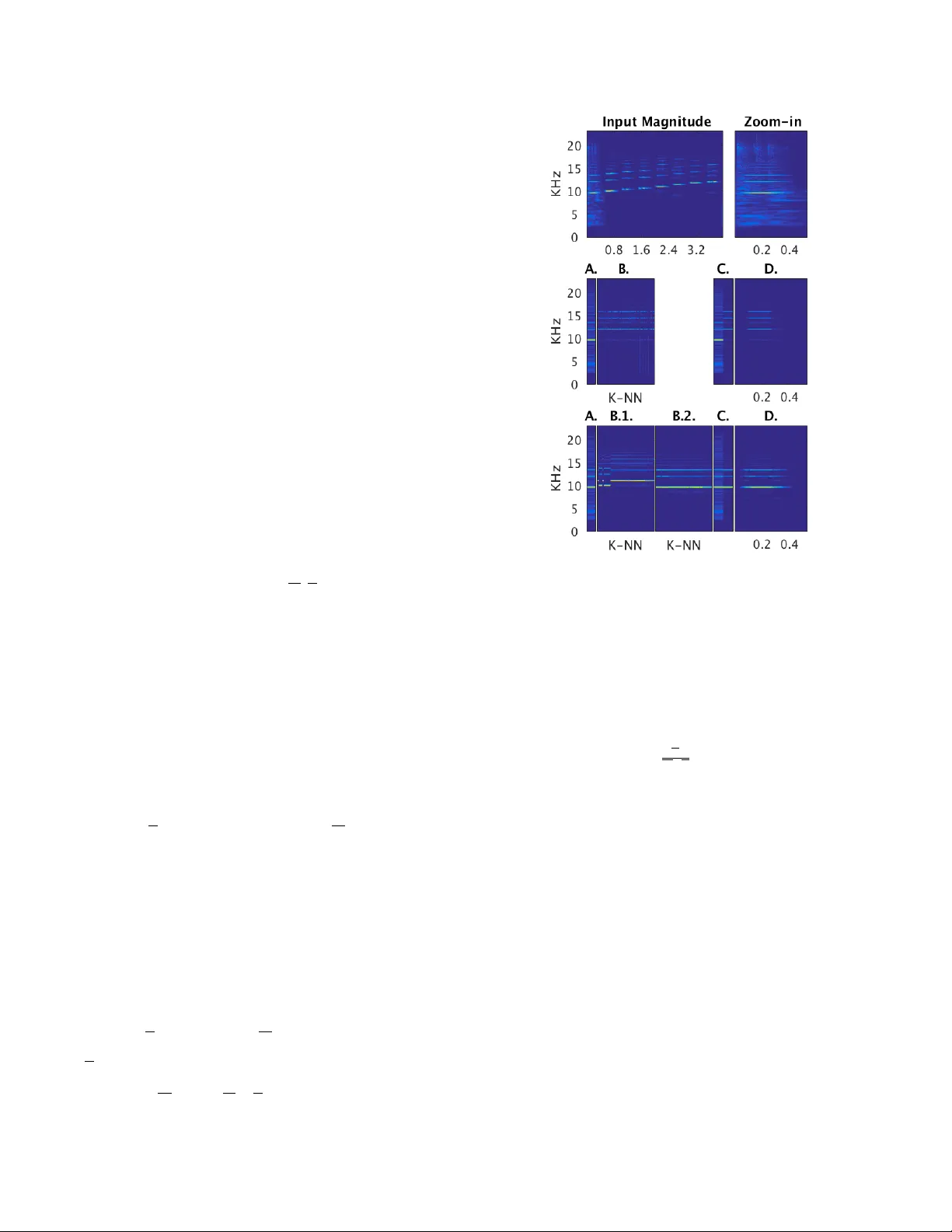
SHIFT -INV ARIANT KERNEL ADDITIVE MODELLING FOR A UDIO SOURCE SEP ARA TION Delia F ano Y ela 1 , Sebastian Ewert 2 , K en O’Hanlon 1 and Mark B. Sandler 1 1 Queen Mary Uni versity of London, UK 2 Spotify ABSTRA CT A major goal in blind source separation to identify and separate sources is to model their inherent characteristics. While most state-of- the-art approaches are supervised methods trained on lar ge datasets, interest in non-data-driv en approaches such as Kernel Additi ve Mod- elling (KAM) remains high due to their interpretability and adaptabil- ity . KAM performs the separation of a giv en source applying rob ust statistics on the time-frequency bins selected by a source-specific kernel function, commonly the K-NN function. This choice assumes that the source of interest repeats in both time and frequency . In prac- tice, this assumption does not always hold. Therefore, we introduce a shift-in variant kernel function capable of identifying similar spectral content e ven under frequenc y shifts. This way , we can considerably increase the amount of suitable sound material available to the rob ust statistics. While this leads to an increase in separation performance, a basic formulation, howe ver , is computationally expensiv e. Therefore, we additionally present acceleration techniques that lower the overall computational complexity . Index T erms — Music Processing, Audio Restoration, Source Separation. 1. INTR ODUCTION Music recordings are typically produced by mixing a lar ge number of instrument tracks, corresponding to vocals, guitars, drums or one of various synthesizers. This process makes analysing and processing music highly challenging as the individual instruments are usually strongly correlated in both time and frequenc y . Spatial information contained in the two stereo channels is often unreliable due to the use of various non-linear sound effects yielding artificial sound scenes which cannot physically be reproduced and are difficult to model. Giv en such constraints, a major goal is to find inherent characteristics of the sources to identify and extract a target. Examples include the temporal behaviour of an instrument (continuity in time [1], vibrato structures [2]) or its spectral characteristics (spectral en velope [3], percussiv e versus harmonic properties [4]). Most state-of-the-art methods are based on either Non-Negati ve Matrix Factorisation (NMF) [5 – 7] or Deep Networks [8], with each having dif ferent trade-of fs with respect to run-time, separation quality and adaptability to new acoustic conditions. Both approaches are widely used in settings where (large amounts of) training material is av ailable, which enables supervised learning and typically yields performance improvements. Howe ver , despite a measurable differ - ence in performance, interest in non-data-driv en methods remains high: a focus on modelling concepts explicitly often increases the interpretability of methods, which opens more angles for including prior knowledge, might help with understanding how data-driv en This w ork w as funded by EPSRC grant EP/L019981/1 and was conducted while S. Ewert was at Queen Mary Univ ersity of London. The authors would like to thank Giulio Moro, Gijs W ijnholds and Adib Mehrabi. methods operate and can lead to a high generalization capacity across datasets. In this context, Kernel Additi ve Modelling (KAM) has been successfully employed for a v ariety of tasks in source separation, such as vocal separation, speech enhancement or interference reduc- tion [9 – 11]. The core idea is related to Gaussian processes (GPs): Giv en a time frequency representation, one makes the assumption that indi vidual entries correlate with others in a known way – in other words, if we can observe the v alue of one entry , we can make a state- ment about the v alue of the related entries. An important dif ference between KAM and GPs is that in the latter an estimate is obtained as a solution of an inference problem, which in volves feedback between values and thus is relati vely slo w . In KAM, feedback does not e xist in this form, which can limit its expressivity on the one hand but allo ws for non-Gaussian relationships, which in practice enables the use of outlier resistant methods from robust statistics, and also leads to a drastic improv ement in terms of computational performance. A central goal in KAM is to design a function (or kernel ) that, giv en a bin in a time-frequency representation, identifies bins ha ving a similar contribution from a gi ven source, ignoring the entries asso- ciated with other sources. If the magnitude of a bin deviates from the remaining ones defined by the kernel, one can assume that another source is present in that bin and that the bins in the kernel can be used to reconstruct the original v alue in the overlaid bin. KAM employs order statistics to attenuate the influence of outliers originating from other sources. A popular kernel choice in KAM is the K nearest neighbours (K-NN) function finding the most similar time frames, based on the squared Euclidean distance [9]. This simple kernel function implicitly relies on two assumptions. Firstly , it assumes the energy in each time frame to be dominated by the source of interest (in [11] the authors present KAM extensions for low SNR conditions). Secondly , using the Euclidean distance between entire frames, the position of partials and other objects cannot change. In other words, frames are required to repeat with only minor modifications. While this might be a valid assumption for full-length pop songs, it might be wrong if the recording is short, the source is consistently overlaid with the same interference in each repetition or for sources with highly variable pitch. In this paper , we propose an extension to the KAM framew ork in the form of a shift-in variant k ernel to ov ercome these limitations. In particular , using a logarithmic frequency axis, our kernel e xtends the K-NN function by comparing not only the original frames but also all shifted versions. In other words, it can identify notes of the same source differing in pitch as similar and reconstruct a unique musical ev ent from them despite the shift. This way , our method drastically increases the sound material av ailable for the sound reconstruction. In a basic version our shift in variant extension is computationally quite expensi ve as distances have to be computed for v arious shifts. There- fore, we present a technique to lo wer the computational complexity and runtime of our proposed kernel considerably: taking inspiration from [12], instead of computing all shifts, we transform our loga- rithmic time-frequency representation into the magnitude specmurt domain, which enables an efficient comparison of frames based on their repetitiv e structures in frequency direction while ignoring the exact location of those structures. This way , we can construct a highly efficient method yielding a pre-selection of frames, which can then easily be pruned. The paper is structured as follows. In Section 2, we describe the baseline version of KAM and our proposed extensions. In Section 3, we apply our proposed method in a studio recording scenario, where the task is to restore short clips of indi vidual instruments and remove interferences such as coughs or door slams. W e conclude in Section 4 with an outlook on future work. 2. PR OPOSED METHOD 2.1. KAM Baseline KAM is a rich framew ork with a wide range of applications [9]. In the following, we limit the description of our baseline approach to the necessary level – our extensions, ho wev er , are just as valid in the full framework. In particular , consider a mixture x ( t ) = s ( t ) + n ( t ) of two different sound sources s and n . W e assume s to be energetically dominant in the mixture and the support of n to be known and be limited to a short duration. For scenarios in which these two assumptions are not met, we refer to [11, 13] for a set of additional KAM extensions. The task is to reco ver s from the gi ven mixture x when n is acti ve. In the follo wing, let X, S ∈ C F × T be time-frequency represen- tations of x and s , respecti vely , and X , S the corresponding magni- tudes. For KAM, we define a similarity kernel function I : F × T → P ( F × T ) that assigns to ev ery time-frequency bin ( f , t ) in S a list of K bins to be called similar (i.e. ∀ ( f , t ) ∈ F × T : |I ( f, t ) | = K ). In the following, the kernel function is the K -nearest neighbours ( K - NN) function based on the squared Euclidean distance. In particular , for ev ery time-frequency bin ( f , t ) , the bin ( f , ˜ t ) will be in I ( f , t ) if the time frame ˜ t is among the K most similar time frames. W ith I ( f , t ) defined, we kno w which bins are similar in S . If a bin in S is ov erlaid by energy corresponding to N , we can use the similar bins in the observed X to identify their commonalities and restore the ov erlaid bin. T o this end, we express this estimation problem in KAM as a minimization of a model cost function L , which can be stated for a single channel as follows: S ( f , t ) ≈ argmin λ ∈ R X ( f , ˜ t ) ∈I ( f ,t ) L ( X ( f , ˜ t ) , λ ) . (1) Depending on the choice of L the information in the bins indexed by I is merged in different w ays. The choice should take into account that, while all these bins are similar in S , there might be considerable, non-Gaussian dif ferences between them in X due to the unknown interference n . A popular choice is L ( a, b ) := | a − b | as it leads to solutions employing operators from robust statistics (order statistics), which enable unbiased parameter estimation in the presence of up to 50% outliers. W ith this choice of L , the solution of the estimation problem (1) is: S ( f , t ) := median( X ( f , ˜ t ) | ( f , ˜ t ) ∈ I ( f , t )) . (2) S being the magnitude estimate of the source of interest s , we define a corresponding magnitude estimate for the remaining sources in the mixture n as N = max( X − S , 0) . Then we can perform the actual separation through soft masking and obtain a complex estimate S of Fig. 1 . Comparison of the baseline (second ro w) and the basic v ersion of our proposed shift-in v ariant method (third row) for an example frame (A) from the input magnitude frames ov erlaid by an interfer- ence (Zoom-in). The K closest frames found for the current frame (A) by the baseline (B) and the proposed method, before (B.1) and after the shifting operation (B.2). The plots (C) contain the current frame next to the estimated output frame for each method. The com- plete estimation of the harmonic source for the frames containing interference is shown in D for both methods. the source of interest via S = S N + S  X , which is con verted to the time-domain using an in verse time-frequency transform. The success of the separation heavily depends on the ability of the kernel to identify similar frames in the presence of overlaying sources. Using just a Euclidean distance between entire frames, this notion of similarity , howe ver , can be quite limited. For example, as it can be seen in the second row of Fig.1, the method might not be able to remove an interference on top of a single note played only once, Fig1.A (as there might be no other similar frames). In particular, the method can not make use of frames where the instrument plays also a note but in a dif ferent pitch – due to the difference in pitch the two frames are likely to be orthogonal, which leads to high differences in the Euclidean distance, as sho wn by the selection of K -NN in Fig1.B. For our comple xity analysis below , note that taking X ∈ C F × T as the input of our system (usually with T > F ), the ov erall com- plexity of this baseline method is O ( T 2 ( F + log T )) . 2.2. Use of the Log-Fr equency Domain KAM implementations typically use a standard linear scale time- frequency representation as it is both memory and computationally inexpensi ve. In such a representation, the spacing between harmonics and fundamental frequency will depend on the latter . Howe ver , using a logarithmic frequency scale the location of e very harmonic with respect to the fundamental frequency will be constant [14]. More precisely , taking f 0 as the fundamental frequency of a signal, the frequency of the n th harmonic will be located at n × f 0 in a linear scale but w ould appear at log f 0 + log n in a logarithmic frequency scale [15]. In particular , within a certain frequency range, pitch shifts simply correspond to shifts in log-frequency representations. 2.3. Shift-In variant KAM For our extension to the baseline kernel we make use of this prop- erty . In particular, let X, S ∈ C F × T be the Constant-Q transform (CQT) of x and s , a log-frequency representation with a perfect reconstruction property [15]. The goal now is to locate not only patterns repeated in time but also their shifted versions. In order to do so, we introduce a shift δ in the kernel function measured in frequency bins. T o this end, let X δ be a frequency shifted version of X: X δ ( f , t ) := X ( f + δ , t ) . W e define our new shift-in variant kernel I s as follows: For a gi ven ( f , t ) , we hav e ( ˜ f , ˜ t ) ∈ I s ( f , t ) if | δ | < ∆ for δ := ˜ f − f and X δ (: , ˜ t ) is among the K closest frames for frame X (: , t ) across all δ ∈ {− ∆ , . . . , ∆ } . Here, we used the slicing notation : to denote all elements in an index dimension. This means that two time frames can no w be considered as neighbours if they display a similar harmonic pattern at different frequenc y loca- tions. In other words, the proposed kernel function I s can be seen as a shift-in variant version of the baseline kernel I . The estimation prob- lem remains essentially the same (just that the v ariability in frequency is now e xplicit): S ( f , t ) ≈ argmin λ ∈ R X ( ˜ f , ˜ t ) ∈I s ( f ,t ) L ( X ( ˜ f , ˜ t ) , λ ) . For the same model cost function as abo ve, we get the solution: S ( f , t ) := median( X ( ˜ f , ˜ t ) | ( ˜ f , ˜ t ) ∈ I s ( f , t )) . As a result of this extension, we can no w recov er a note played only once by using notes different in pitch played by the same instrument, as seen in the third row of Fig1. In practice, the implementation of this approach can be split into two main steps: similarity measure (Fig1.B.1) and frequency alignment (Fig1.B.2). In particular, e very frame in the mixture has to be shifted in frequenc y direction and compared to the remaining frames, 2 · ∆ times. Computing the Euclidean distances in ev ery step is in O ( T 2 · F ) . All together , with ∆ typically being dependent on F , the comple xity of this approach is considerable: O ( T 2 ( F 2 + log T )) . In practice, even after limiting ∆ to a reasonable frequency range (such as 1-2 octav es), a basic implementation of this approach turns out to be computationally quite expensi ve. 2.4. Acceleration Extension Under runtime constraints, the method above forces the user to trade- off separation performance for better running time. For e xample, one may set the ∆ to cov er only half an octav e, at the risk of not finding similar e vents. In this section, we describe techniques to accelerate the kernel defined in Section 2.3 considerably , while preserving the increase in separation quality . 2.4.1. Similarity measur e Instead of applying the kernel function on the magnitude of the CQT , we propose to use a different time-frequenc y representation to allow a quicker shift-in variant search. The idea it to employ a representa- tion that captures the (harmonic) patterns in each frame, while being in variant against their exact location. More precisely , giv en the mag- nitude CQT X , we perform our search on the magnitude spectrum calculated on each frame X (: , t ) . This transform is related to cepstral analysis [16] but has more recently been called specmurt analysis [12] when applied to a log-frequency linear-magnitude representation (as in our case). Using the specmurt domain brings v arious advantages. First, eliminating the specmurt-phase, we eliminate pitch information and keep only the ’pattern’ information. Second, certain spectral char- acteristics are represented more compactly . For example, a broad- band sound in the time-frequency domain will correspond to ’lo w- frequency’ components in the specmurt domain. This way , percus- siv e components can more easily be ignored in the similarity search (if needed) and provides an interesting ne w angle to design source specific kernels by applying dif ferent weightings to the specmurt coefficients. Further , we can exploit the symmetry of the Fourier transform to eliminate half of the specmurt components, reducing the run time further . Overall, instead of O ( T 2 ( F 2 + log T )) operations for the shifts and Euclidean distances as before, we transform X to specmurt and only hav e to perform one set of Euclidean distances (comparable to the baseline that does not support shift in variance), resulting in only O ( T 2 ( F + log T )) operations for these steps. 2.4.2. F requency Alignment While the approach in Section 2.4.1 enables a rapid shift-inv ariant selection of frames, it does not provide the shift we need to apply to a frame such that it is indeed similar to a given one. Given an input frame, a first idea is to apply all possible shifts to the K frames found as similar on the specmurt domain. While this is a considerable speedup over the plain approach described in Section 2.3, it is still rather slow . Therefore, we will accelerate this step next, ag ain using the Fourier transform, which w as explored in [12] in a related form in the context of source-filter modelling. T o this end, we assume we kno w from the last step that frames t and ˜ t are similar . For notational purposes, we will use the shorthands Y := ˜ X (: , t ) and Z := ˜ X (: , ˜ t ) . That means, Y and Z differ mostly by a shift in frequency , which we need to identify . W e can express this as Y = H ∗ Z and solve for H – in case Y = Z , H (0) = 1 and there is no shift. If all entries in Z are shifted by 1 compared to Y , we obtain H (1) = 1 . That means, to obtain the correct shift between Y and Z we only need to compute a decon volution between them – and the Fourier transform can again accelerate this step. As detailed in [12], a fast decon volution can be calculated via H = F  I F ( Y ) I F ( Z )  , (3) where I F and F denote the (inv erse) Fourier transform. Assuming that frames t and ˜ t are indeed similar , the H we obtain this way , will typically be very sparse and essentially hav e a strong peak at exactly one position, which indicates the shift we need to apply to frame ˜ t . Once we hav e the optimal shift for all K close frames we can continue as in the baseline method. Combining the two acceleration methods, the computational comple xity is O ( T 2 ( F + log T )) + O ( T · F log F ) . 2.4.3. Pruning Even though measuring similarity based on the magnitude specmurt considerably reduces the computational comple xity , it does not assure the frames found to be similar are the most similar . Discarding the phase in the kernel function renders the method shift-in variant but it also eliminates the unitary property of the F ourier Transform, i.e. Parsev al’ s theorem does not hold anymore and thus Euclidean distances can be different. Therefore, when measuring the Euclidean distance between two frames in the magnitude specmurt, a large distance certainly indicates dissimilarity but a small distance does not assure a close match in the time-frequency domain (for example, major and minor chords can get confused). T o ov ercome this drawback while maintaining the complexity reduction, we here propose to use our acceleration technique as a pruning method. Instead of selecting K-NN in the kernel function, we select a larger fix ed value ( K + P ) to increase the pool of close frames. W e then perform the specmurt analysis described above to find their optimal shift. At this point, one can retrieve these ( K + P ) frames in the time-frequency representation and shift them by their corresponding amount. This means, we now ha ve a narro wed down shifted version of the input magnitude, and so we can apply the baseline method to select the K-NN from the ( K + P ) frames presented. The overall comple xity remains the same. 3. EV ALU A TION W e e valuated the proposed method for an interference reduction application, where a b urst-like sound ov erlays the audio recording. In particular , we focused on four different interferences that typically occur in liv e or studio recording scenarios: cough, chair drag sound, door slam and sound of object being dropped. W e retrie ved example recordings of each from freesound.org . In the follo wing, we are mainly interesting in finding out how the different methods beha ve on recordings where the musical source is not repeated in time. T o this end, we created a synthetic dataset where the repeated and not repeated passages are kno wn, so that we were able to compare the proposed method against the baseline in both cases. W e created five different melodies (monophonic) and fiv e different chord progressions, to simulate short studio takes, and synthesized these with 12 different instruments using the high quality Nativ e Instruments Komplete Ultimate suite. W e then created test recordings by ov erlaying the recordings with the interferences at 12 dB SNR, placing the interferences at two different locations: on a repeated musical se gment and on a not repeated one, resulting on 960 tracks between 5 and 10 seconds each. While a more realistic dataset might better indicate the performance of the methods, we chose this setup to in vestigate e xactly those cases where the individual methods might differ the most. T o quantitati vely compare the separation quality of our proposed extension to the baseline, we used the BSS Ev al toolbox 3.0 [17] to calculate the Signal to Distortion Ratio (SDR). W e used the CQT implementation described in [15], setting the parameters to 24 bins per octave, gamma value of 20, minimum frequency of 27.5Hz and the maximum frequenc y being half of the sampling frequency (44.1KHz). For all methods, we set the parameter K of the K -NN kernel function to 300 frames. Note howe ver , that K can and should be adjusted to the level of repetitiveness in the input recordings – the higher the repetitiv eness, the more all methods benefit from higher K . For our proposed method, we fixed the number of shifts ∆ to 48 (cov ering 4 octav es in total). In the acceleration+pruning method, the parameter P of the ( K + P ) − N N kernel function is set to be 2 K . W e ignored the first coefficient in the specmurt representation as we expect it to mainly capture the broadband components. In addition, we assume the location of the interference in the mixture is known (and refer to [11] otherwise) and thus we only process the frames af fected and Melody Chords Repeated Not repeated Repeated Not repeated Baseline 3.31 -2.40 4.11 1.26 Prop. 01 4.61 3.87 4.11 2 . 11 Prop. 02 5.06 4.22 4.03 1.09 Prop. 03 5 . 23 4 . 36 4 . 52 2.10 T able 1 . NSDR values for the baseline, the basic shift-inv ariant proposed method (Prop. 01) and the acceleration technique without pruning (Prop.02) and with pruning from an initial pool of twice the amount of K frames (Prop. 03). Parameters: K = 300, SNR = 12dB, ∆ = 48 measure the SDR on those segments. The kernel function for all methods is applied to the remainder of the frames. The results with respect to the normalised SDR (NSDR) are giv en in T able 1, for both melody and chord progressions, on re- peated and not repeated musical segments. As expected, the KAM baseline behaves poorly when there is no repetition, especially for melodies, which resembles the common scenario in popular songs where the source of interest is consistently repeating on the same pattern of unwanted sources. The NSDR value for the baseline for the non-repeated chords shows that, even though the chord is not repeated, some of its notes might, which can already be exploited by the method. Howev er, the basic shift-inv ariant method ( P rop. 01 ) clearly outperforms the baseline in those not repeated cases demon- strating standard KAM’ s limitations in such cases. In addition, it matches or improves the performance of the baseline on repeated segments, which suggests the proposed kernel function benefits from the shifting operation presenting the overlaying unwanted sources as clear outliers (affected by a shift in frequency). The basic shift- in variant method remains computationally e xpensiv e. Howe ver , the proposed methods based on specmurt analysis with ( P rop. 03 ) and without pruning ( P rop. 02 ) are ef fectiv e in the melody scenario by ev en improving upon P rop. 01 ’ s separation performance. This can be e xplained by the fact that the accelerated v ariants can find arbitrary shifts, while the shift in P rop. 01 is limited to reduce the compu- tational time. In the chord progressions scenario, the lo w results of P rop. 02 confirms limitations in using the specmurt domain and justifies its use as a pre-selector for the pruning method P rop. 03 . 4. CONCLUSION W e ha ve presented an e xtension to the KAM framew ork in the form of a shift-in v ariant kernel function, aiming to overcome KAM’ s limi- tations with respect to non-repeating musical passages of the source of interest. W e introduced a frequency shift in the kernel function to incorporate instances of the source of interest with similar frequency pattern at different frequenc y locations, increasing the pool of similar frames av ailable for the source’ s reconstruction. Firstly we described a basic implementation bearing a high computational complexity and then presented acceleration techniques, which considerably lowered the computational complexity and runtime. The proposed methods were ev aluated in an interference reduction scenario for transient noise typically found on li ve and studio music recordings. The results clearly demonstrate the inability of the baseline kernel to reconstruct non-repeated musical e vents and confirms the ef ficacy of the proposed shift-in variant kernel for such cases. Ho wev er, e ven for repeated seg- ments, the increase of the pool of similar frames led to improv ements ov er standard KAM. Possible future directions for extending this work include an implementation for naturally sparse sources such as vocals. 5. REFERENCES [1] T uomas V irtanen, “Monaural sound source separation by nonnegati ve matrix factorization with temporal continuity and sparseness criteria, ” IEEE T ransactions on Audio, Speech and Language Pr ocessing , vol. 15, no. 3, pp. 1066–1074, 2007. [2] Lise Regnier and Geof froy Peeters, “Singing voice detection in music tracks using direct voice vibrato detection, ” in Pr o- ceedings of the IEEE International Confer ence on Acoustics, Speech, and Signal Pr ocessing (ICASSP) , T aipei, T aiwan, 2009, pp. 1685–1688. [3] Jean-Louis Durrieu, Ga ¨ el Richard, Bertrand David, and C ´ edric F ´ evotte, “Source/filter model for unsupervised main melody extraction from polyphonic audio signals, ” IEEE T ransactions on Audio, Speech and Language Pr ocessing , vol. 18, no. 3, pp. 564–575, 2010. [4] Nobutaka Ono, Kenichi Miyamoto, Jonathan LeRoux, Hirokazu Kameoka, and Shigeki Sagayama, “Separation of a monaural audio signal into harmonic/percussive components by com- plementary diffusion on spectrogram, ” in Proceedings of the Eur opean Signal Processing Conference (EUSIPCO) , 2008, pp. 240–244. [5] Mikkel N. Schmidt and Morten Mørup, “Nonnegati ve matrix factor 2-D deconv olution for blind single channel source sep- aration, ” in Pr oceedings of the International Conference on Independent Component Analysis and Blind Signal Separation . 2006, pp. 700–707, Springer Berlin/Heidelberg. [6] Paris Smaragdis, Bhiksha Raj, and Madhusudana Shashanka, “Sparse and shift-inv ariant feature extraction from non-negativ e data, ” in Proceedings of the IEEE International Conference on Acoustics, Speech, and Signal Pr ocessing (ICASSP) , Las V e gas, Nev ada, USA, 2008, pp. 2069–2072. [7] Alex ey Ozero v , Emmanuel V incent, and Fr ´ ed ´ eric Bimbot, “ A general flexible frame work for the handling of prior informa- tion in audio source separation, ” IEEE T ransactions on Audio, Speech, and Language Processing , vol. 20, no. 4, pp. 1118– 1133, 2012. [8] Stefan Uhlich, Franck Giron, and Y uki Mitsufuji, “Deep neural network based instrument e xtraction from music, ” in Proceed- ings of the IEEE International Confer ence on Acoustics, Speech and Signal Pr ocessing (ICASSP) , 2015, pp. 2135–2139. [9] Antoine Liutkus, Derry FitzGerald, Zafar Rafii, Bryan Pardo, and Laurent Daudet, “Kernel additi ve models for source separa- tion, ” IEEE T ransactions on Signal Processing , v ol. 62, no. 16, pp. 4298–4310, 2014. [10] Zafar Rafii and Bryan Pardo, “Online REPET -SIM for real-time speech enhancement, ” in Proceedings of the IEEE Interna- tional Confer ence on Acoustics, Speech and Signal Pr ocessing (ICASSP) , 2013, pp. 848–852. [11] Delia Fano Y ela, Sebastian Ewert, Derry FitzGerald, and Mark B. Sandler , “Interference reduction in music recordings combining kernel additi ve modelling and non-negati ve matrix factorization, ” in Pr oceedings of the IEEE International Con- fer ence on Acoustics, Speech, and Signal Processing (ICASSP) , 2017, pp. 51–55. [12] Shoichiro Saito, Hirokazu Kameoka, Keigo T akahashi, T akuya Nishimoto, and Shigeki Sagayama, “Specmurt analysis of poly- phonic music signals, ” IEEE T ransactions on Audio, Speech, and Language Pr ocessing , vol. 16, no. 3, pp. 639–650, 2008. [13] Delia Fano Y ela, Sebastian Ewert, Derry Fitzgerald, and Mark Sandler , “On the importance of temporal context in proximity kernels: A vocal separation case study , ” in Audio Engineering Society Confer ence: 2017 AES International Conference on Semantic Audio , Jun 2017. [14] Judith C. Bro wn, “Calculation of a constant Q spectral trans- form, ” Journal of the Acoustical Society of America , vol. 89, no. 1, pp. 425–434, 1991. [15] Christian Sch ¨ orkhuber , Anssi Klapuri, Nicki Holighaus, and Monika D ¨ orfler , “ A matlab toolbox for ef ficient perfect recon- struction time-frequency transforms with log-frequency resolu- tion, ” in Pr oceedings of the International A udio Engineering Society Confer ence: Semantic Audio , 2014. [16] Lawrence Rabiner and Bing-Hwang Juang, Fundamentals of Speech Recognition , Prentice Hall Signal Processing Series, 1993. [17] Emmanuel V incent, R ´ emi Gribon v al, and C ´ edric F ´ evotte, “Per- formance measurement in blind audio source separation, ” IEEE T ransactions on Audio, Speech, and Language Pr ocessing , vol. 14, no. 4, pp. 1462–1469, 2006.