Reconditioning your quantile function

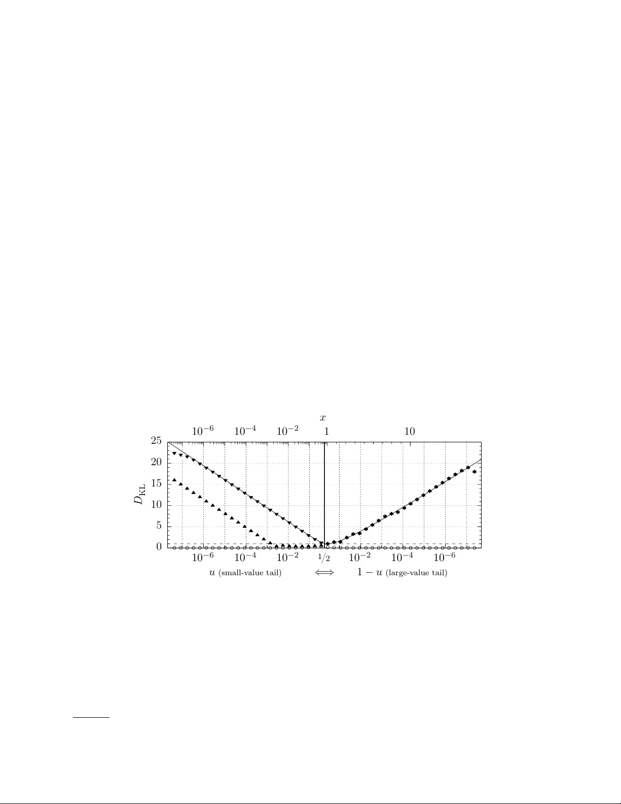
Reconditioning y our quan tile function Keith P edersen ∗ Il linois Institute of T e chnolo gy, Chic ago, IL 60616 Mon te Carlo sim ulation is an imp ortan t to ol for mo deling highly nonlinear systems (like particle colliders and cellular mem branes), and random, floating-p oin t num bers are their fuel. These random samples are frequently generated via the inv ersion metho d, which harnesses the mapping of the quan tile function Q ( u ) (e.g. to generate prop osal v ariates for rejection sampling). Y et the increasingly large sample size of these simulations mak es them vulnerable to a fla w in the in version method; Q ( u ) is il l-c onditione d in a distribution’s tails, stripping precision from its sample. This flaw stems from limitations in machine arithmetic whic h are often o verlooked during implementation (e.g. in p opular C++ and Python libraries). This pap er introduces a r obust inv ersion metho d, which reconditions Q ( u ) by carefully drawing and using uniform v ariates. pqRand , a free C++ and Python pack age, implements this nov el metho d for a num b er of p opular distributions (exp onen tial, normal, gamma, and more). INTR ODUCTION The in version metho d samples from a probability distribution f via its quantile function Q ≡ F − 1 , the in verse of f ’s cum ulative distribution F [1, 2]. Q is used to transform a random sample from U (0 , 1) , the uniform distribution ov er the unit interv al, into a random sample { f } ; { f } = Q  { U (0 , 1) }  . (1) This sc heme is p o w erful b ecause quan tile functions are formally exact. But an y real-world im- plemen tation will b e formal ly inexact b ecause: (i) A source of true randomness is generally not practical (or even desirable), while a rep eatable pseudo-random num b er generator (PRNG) is never p erfect. (ii) The uniform v ariates u and their mapping Q ( u ) use finite-precision machine arithmetic. The first defect has received the lion’s share of atten tion, leaving the second largely ignored. As a result, common implementations of inv ersion sampling lose precision in the tails of f . This leak must b e subtle if no one has patched it. Nonetheless, the loss of precision commonly exceeds dozens of ULP (units in the last place) in a distribution’s tails. Con trast this to library math functions ( sin , exp ), whic h are painstakingly crafted to deliver no more than one ULP of systematic error. When the inv ersion metho d loses precision, it pro duces inferior, rep etitiv e samples, to which Mon te Carlo sim ulations may b ecome sensitive as they gro w more complex, drawing ever more random num bers. Proving that the effect is negligible is incredibly difficult, so the b est alternative is to use the most numerically stable sampling scheme p ossible with floating p oin t n umbers — if it is not to o slow. The robust inv ersion metho d prop osed here is 80–100% as fast as the original. T o isolate the loss of precision, we examine the three indep enden t steps of inv ersion sampling: 1. Generate random bits (i.i.d. coin flips) using a PRNG. 2. Con v ert those random bits into a uniform v ariate u from U (0 , 1) . 3. Plug u in to Q ( u ) to sample from the distribution f . The first t wo steps do not dep end on f , so they are totally generic (a ma jor virtue of the metho d). Of them, step 1 has b een exhaustively studied [3–5], and is essen tially a solved problem — when in doubt, use the Mersenne t wister [5, 6]. Step 3 has b een v alidated using real analysis [1, 7], so that kno wn quan tile functions need only b e translated into computer math functions. ∗ kp eders1@ha wk.iit.edu 2 This leav es step 2 whic h, at first glance, lo oks like a trivial co ding task to p ort random bits into a real-v alued Q . Y et computers cannot use real n umbers, and neglecting this fact is dangerous — using this as its central maxim, this pap er conducts a careful inv estigation of the inv ersion metho d from step 2 on ward. Section I b egins by using the condition n umber to prob e step 3, finding that a distribution’s quantile function is numerically unstable in its tails. This provides a sound framework for Sec. I I to find the subtle flaw in the canonical algorithm for dra wing uniform v ariates (step 2). A r obust inv ersion metho d is introduced to fix b oth problems, and is empirically v alidated in Sec. I I I b y comparing the near-p erfect sample obtained from the pqRand pac k age to the deficient samples obtained from standard C++ and Python to ols. I. Q ARE ILL-CONDITIONED, BUT THEY DO NOT HA VE TO BE Real num bers are not countable, so computers cannot represen t them. Mac hine arithmetic is limited to a countable set lik e rational num bers Q . The most v ersatile rational approximation of R are flo ating p oint num bers, or “floats” — scien tific notation in base-tw o ( m × 2 E ) . The precision of floats is limited to P , the n um b er of binary digits in their mantissa m , which forces relative rounding errors of order  ≡ 2 − P up on ev ery floating p oin t operation [8]. The propagation of suc h errors makes floating p oint arithmetic formally inexact. In the w orst case, subtle effects like cancellation can degrade the effe ctive (or de facto) precision to just a handful of digits. Using floats with arbitrarily high P mitigates such problems, but is usually em ulated in softw are — an exp ensiv e cure. Prudence usually restricts calculations to the largest precision widely supp orted in hardw are, binary64 ( P = 53 ), commonly called “double” precision. Limited P makes the intrinsic stability of a computation an imp ortant consideration; a result should not change dramatically when its input suffers from a pinch of rounding error. The numerical stabilit y of a function g ( x ) can b e quantified via its condition num ber C ( g ) — the relativ e c hange in g ( x ) p er the relativ e c hange in x [9] C ( g ) ≡     g ( x + δ x ) − g ( x ) g ( x ) . δ x x     =     x g 0 ( x ) g ( x )     + O ( δ x ) . (2) When an O (  ) rounding error causes x to increment to the next representable v alue, g ( x ) will incremen t by C ( g ) representable v alues. So when C ( g ) is large (i.e. log 2 C ( g ) → P ), g ( x ) is il l- c onditione d and imprecise; the tiniest shift in x will cause g ( x ) to hop o v er an enormous num ber of v alues — v alues through which the real-v alued function passes, and whic h are represen table with floats of precision P , but which cannot b e attained via the floating p oint calculation g ( x ) . The condition num b er should b e used to av oid such numerical catastrophes. W e no w hav e a to ol to uncov er p ossible instability in the inv ersion metho d, sp ecifically in its quan tile function Q (step 3). As a case study , w e can examine the exp onential distribution (the time b et ween ev ents in a Poisson pro cess with rate λ , lik e radioactiv e deca y); 1 f ( x ) = λ e − λx − → F ( x ) = 1 − e − λx ; (3) Q 1 ( u ) = − 1 λ log(1 − u ) = − 1 λ log1p ( − u ) − → C ( Q 1 ) = − u (1 − u ) log1p ( − u ) . (4) A well-conditioned sample from the exp onential distribution will require C ( Q 1 ) ≤ O (1) ev erywhere, but Fig. 1a clearly reveals that C ( Q 1 ) (dashed) b ecomes large as u → 1 . Wh y is Q 1 ill-conditioned there? A ccording to Eq. 2, a function can b ecome ill-conditioned when it is ste ep ( | g 0 /g |  1) , and 1 log1p ( x ) is an implemen tation of log(1 + x ) which sidesteps an unnecessary floating p oint cancellation [10]. 3 Q 1 (solid) is clearly steep at b oth u = 0 and u = 1 . These are f ’s “tails” — a large range of sample space mapp ed by a thin, low probability slice of the unit in terv al. Y et in spite of its steepness, Q 1 remains well-conditioned throughout its small-v alue tail ( u → 0 ) b ecause floats are denser near the origin — reusing the same set of man tissae, but with smaller exp onents — and a denser set of u allo ws a more contin uous sampling of a rapidly c hanging Q 1 ( u ) . This extra densit y manifests as the singularity-softening factor of x in Eq. 2. Unfortunately , the same relief cannot o ccur as u → 1 , where representable u are not dense enough to accommo date Q 1 ’s massive slop e. 1 10 − 3 10 − 2 10 − 1 10 1 0 0.2 0.4 0.6 0.8 1 x u Q 1 ( u ) C ( Q 1 ) (a) 1 10 − 3 10 − 2 10 − 1 10 1 1 / 2 1 10 − 2 10 − 1 x u Q 1 ( u ) C ( Q 1 ) Q 2 ( u ) C ( Q 2 ) (b) FIG. 1: The λ = 1 exp onential distribution f ( x ) = e − x ; (a) the quantile function Q 1 (solid) and its condition num ber (dashed) and (b) the “quan tile flip-flop” — in the domain 0 < u ≤ 1 / 2 , eac h Q maps out half of f ’s sample space while remaining w ell-conditioned. Because Q 1 is ill-conditioned near u = 1 , the large- x p ortion of its sample { f } will b e imprecise; man y large- x floats which should b e sampled are skipp ed-ov er by Q 1 . This problem is not unique to the exp onential distribution; it will o ccur whenev er f has tw o tails, b ecause one of those tails will b e lo cated near u = 1 . Luc kily , U (0 , 1) is p erfectly symmetric across the unit in terv al, so transforming u 7→ 1 − u pro duces an equally v alid quantile function; Q 2 ( u ) = − 1 λ log( u ) − → C ( Q 2 ) = − 1 log( u ) . (5) The virtue of using tw o v alid Q ’s is evident in Fig. 1b; for u ≤ 1 / 2 , each version is well-conditioned, with Q 1 sampling the small-v alue tail ( x ≤ median ) and Q 2 the large-v alue tail ( x ≥ median ) . Since the pair collectively and stably spans f ’s en tire sample space, f can b e sampled via the comp osition metho d; for each v ariate, randomly choose one version of the quantile function (to av oid a high/low pattern), then feed that Q a random u from U (0 , 1 / 2 ] . This “quan tile flip-flop” — a randomized, tw o- Q comp osition split at the median — is a simple, general scheme to recondition a quan tile function which b ecomes unstable as u → 1 . It is also immediately p ortable to antithetic v ariance reduction, a useful technique in Mon te Carlo in tegration where, for ev ery x = Q ( u ) one also includes the opp osite c hoice x 0 = Q ( u 0 ) [11]. A common con ven tion is u 0 ≡ 1 − u , which can create a negativ e cov ariance co v ( x, x 0 ) that decreases the ov erall v ariance of the integral estimate. Generating antithetic v ariates with a quantile flip-flop is trivial; instead of randomly choosing Q 1 or Q 2 for each v ariate, alwa ys use b oth. 4 I I. AN OPTIMALL Y UNIFORM V ARIA TE IS MAXIMALL Y UNEVEN The condition n umber guided the dev elopment of the quan tile flip-flop, a rather simple wa y to stabilize step 3 of the inv ersion metho d during machine implementation. Our inv estigation now pro ceeds to step 2 — sampling uniform v ariates. While steps 2 and 3 seem indep endent, we will find that there is an imp ortant interpla y b etw een them; a quan tile function can b e destabilized b y sub-optimal uniform v ariates, but it can also wreck itself by mishandling optimal uniform v ariates. The canonical metho d for generating uniform v ariates is Alg. 1 [2–4, 10, 12–15]; an in teger is randomly dra wn from [0 , 2 B ) , then scaled to a float in the half-op en unit interv al [0 , 1) . Using B ≤ P produces a completely uniform sample space — each p ossible u has the same probabilit y , with a rigidly even spacing of 2 − B b et ween eac h. Using B = P gives the ultimate even sample { U E [0 , 1) } , as depicted in Fig. 2E (which uses a ridiculously small B = P = 4 to aide the eye). When B > P , line 4 will b e forced to round man y large j , as the mantissa of a is not large enough to store ev ery j with full precision. As B → ∞ , this rounding saturates the floats av ailable in U [0 , 1) , creating the uneven { U N [0 , 1) } depicted Fig. 2N. This uneven sample space is still uniform b ecause large u are more probable, absorbing more j from rounding (due to their coarser spacing). Algorithm 1 Canonically draw a random float (with precision P ) uniformly from U [0 , 1) Require: B ∈ Z +  B must b e a p ositiv e in teger 1: A ← flo a t (2 B )  Conv ert 2 B = ( j max + 1) to a float (a p ow er-of-t wo gets an exact conv ersion). 2: rep eat 3: j ← RNG ( B )  Draw B random bits and conv ert them into a integer from U [0 , 2 B ) . 4: a ← floa t ( j )  Conv ert j to a float with precision P . Rounding ma y o ccur if j > 2 P . 5: until a < A  If B > P and j rounds to A , the algorithm should not return 1. 6: return a/ A 0.0 0.2 0.4 0.6 0.8 1.0 (E) ev en; B = P . 0.0 0.2 0.4 0.6 0.8 1.0 (N) unev en; B → ∞ . FIG. 2: A visual depiction (using floats with P = 4 for clarity) of eac h p ossible u for (E) even { U E [0 , 1) } and (N) uneven { U N [0 , 1) } . The heigh t of each tic indicates its relativ e probabilit y , which is prop ortional to the width of the num ber-line segment which rounds to it. Dep ending on the c hoice of B , Alg. 1 can generate uniform v ariates whic h are either even or unev en, but which is b etter? There seem to b e no definitive answers in the literature — which is lik ely why different implemen tations choose different B — so w e will hav e to find our o wn answ er. W e start by c ho osing the even uniform v ariate { U E [0 , 1) } as the null h yp othesis, for tw o obvious reasons: (i) Fig. 2E certainly lo oks more uniform and (ii) taking B → ∞ do es not seem practical. Ho wev er, we will so on find that p erfect evenness has a subtle side effect — it forces all quan tile functions to b ecome ill-conditioned as u → 0 , even if they ha ve an excellent condition num ber! The condition num ber implicitly assumes that δ x is v anishingly small. This is true enough for a generic float, whose δ x = O (  x ) is m uch small than x . But the ev en uniform v ariates hav e an absolute spacing of δ u =  . T o account for a finite δ x , we define a function’s effe ctive precision P ∗ ( g ) ≡     g ( x + δ x ) − g ( x ) g ( x )     = δ x     g 0 ( x ) g ( x )     + O ( δ x 2 ) . (6) 5 Lik e C ( g ) , a large effective precision P ∗ ( g ) indicates an ill-conditioned calculation. F or a generic floating p oin t calculation δ x = O (  x ) , so P ∗ rev erts bac k to the condition num b er ( P ∗ ( g ) ≈  C ( g ) ). But feeding even uniform v ariates in to a quan tile function giv es δ u =  , so P ∗ E ( Q ) =      Q 0 ( u ) Q ( u )     + O (  2 ) . (7) Calculating P ∗ E ( Q ) for the quantile flip-flop of Fig. 1b indicates that b oth Q b ecome ill-conditioned as u → 0 (where Q b ecomes steep), in stark opp osition to their excellent condition num bers. That using even uniform v ariates will break a quan tile flip-flop is a problem not unique to the exp onential distribution; it o ccurs whenever f has a tail (so that | Q 0 /Q | → ∞ as u → 0 ). The reduced effective precision P ∗ E ( Q ) caused by ev en uniform v ariates creates sparsely p opulated tails; there are many extreme v alues which { f } will nev er contain, and those whic h it do es will b e sampled to o often. { U E [0 , 1) } is simply to o finite ; 2 P ev en uniform v ariates can supply no more than 2 P unique v alues. This implies that the uneven sample { U N [0 , 1) } will restore quantile stabilit y , since its denser input space ( δ u = O ( u ) ) will stabilize P ∗ N ( Q ) near the origin. These small u expand the sample space of { f } many times ov er, making its tails far less repetitive. And since unev en v ariates corresp ond to the limit where B → ∞ in Alg. 1, they are equiv alen t to sampling U [0 , 1 −  ) from R and rounding to the nearest float — the next b est thing to a real-v alued input for Q . The virtue of using uneven uniform v ariates also follo ws from information theory . The Shannon en tropy of a sample space X counts ho w man y bits of information are conv ey ed by each v ariate x ; H ( X ) ≡ − X i Pr( x i ) log 2 Pr( x i ) . (8) The sample space of the ev en uniform v ariates ( B = P ) has n =  − 1 equiprobable members, so H E = − n X i =1  log 2 (  ) = − log 2  = P . (9) This makes sense, since each ev en uniform v ariate originates from a P -bit pseudo-random in teger. The sample space of the uneven { U N [0 , 1) } con tains ev ery float in [0 , 1) , which is naturally partitioned into sub-domains [2 − k , 2 − k +1 ) with common exp onent − k . Each domain comprises a fraction 2 − k of the unit interv al, and the minimum exp onent − K dep ends on the floating p oint t yp e (although K  1 for binary32 and binary64 ). The uneven entrop y is then the sum ov er sub-domains, each of which sums o v er the n/ 2 equiprobable mantissae 2 H N = − K X k =1   n/ 2 X i =1 2 − k (2  ) log 2  2 − k (2  )    = K X k =1 2 − k ( P − 1 + k ) ≈ P + 1 ( for K  1) . (10) One mor e bit of information than even v ariates is not a windfall. But H E and H N are the entropies of the bulk sample { U [0 , 1) } . What is the entrop y of the tail-sampling sub-space U [0 , 2 − k ) ? Rejecting all u ≥ 2 − k in the ev en sample { U E [0 , 1) } , we find that smaller u ha v e less information H E ( k ) = P − k ( for u < 2 − k ) . (11) This lack of information in even v ariates is inevitably mapp ed to the sample { f } , consistent with the deteriorating effective precision as u → 0 . But for uneven uniform v ariates, the sample space is 2 Ignoring the fact that exact pow ers of 2 are 3 / 4 as probable, which mak es no difference once P & 10 . 6 fr actal ; each sub-space lo oks the same as the whole unit interv al, so that H N ( k ) = P + 1 as b efore! Ev ery u has maximal information, and a high-en trop y input should give a high-precision sample. Both the effectiv e precision P ∗ ( Q ) and Shannon en trop y H predict that using even uniform v ariates will force a well-conditioned quantile function to b ecome ill-conditioned, precluding a high- precision sample. Switching to unev en uniform v ariates will r e c ondition it. But there is an imp ortant ca veat; uneven v ariates are very delicate. Subtracting them from one mutates them back into even v ariates (with opp osite b oundary conditions); 1 − { U N [0 , 1) } 7→ { U E (0 , 1] } . (12) This is floating p oint c anc el lation . The subtraction erases an y extra density in the unev en sample, b ecause it maps the very dense region (near zero) to a region where floats are intrinsically sparse (near one). Con versely , the sparse region of the uneven sample (near one) has no extra information to conv ey when it is mapp ed near zero, and remains sparse. This is wh y Q 1 (Eq. 4) must use log1p . I I I. PRECISION: LOST AND F OUND In Sec. I we conditioned an intrinsically imprecise quantile function using a t wo- Q comp osition. Then in Sec. I I w e determined that uneven uniform v ariates are required to ke ep Q w ell-conditioned. These t wo practices comprise our r obust in v ersion metho d, whose technical details we hav e delib- erately left for the App endix b ecause we hav e yet to prov e that it makes a material difference. If indiscreet sampling decimates the precision of { f } , it should b e quite eviden t in an exp eriment! The quality of a real-world sample { f } can b e assessed via its Kullback-Leibler divergence [16] D KL ( b P || b Q ) = X i b P ( x i ) log 2 b P ( x i ) b Q ( x i ) . (13) D KL quan tifies the r elative entrop y b etw een a p osterior distribution b P and a prior distribution b Q (c.f. Eq. 8). The empirical b P is based on the count c i — the num ber of times x i app ears in { f } b P ( x i ) = c i / N (14) (where N is the sample size). The ide al density b Q is obtained by mapping f onto floats, using the domain of real num bers ( x i,L , x i,R ) that round to each x i ; b Q ( x i ) = Z x i,R x i,L f ( x ) d x = F ( x i,R ) − F ( x i,L ) . (15) D KL do es not sum terms where b P ( x i ) = 0 (i.e. x i w as not drawn), b ecause lim x → 0 x log x = 0 . The D KL div ergence is not a metric b ecause it is not symmetric under exc hange of b P and b Q [16]. And while D KL is frequen tly interpreted as the information gaine d when using distribution b P instead of b Q , this is not true here. Consider a PRNG whic h samples from b Q = U (0 , 1) , but samples so p o orly that it alw ays outputs x = 0 . 5 (and th us emits zero information). Its D KL ≈ P is clearly the precision lost b y b P (the generator). In less extreme cases, since b Q is the most precise distribution p ossible giv en floats of precision P , any div ergence denotes ho w man y bits of precision were lost . Our exp eriments calculate D K L for samples of the λ = 1 exp onential distribution generated via the inv ersion metho d. W e use GNU’s std::mt19937 for our PRNG ( B = 32 ), fully seeding its state from the computer’s en vironmental noise (using GNU’s std::random_device ). Calculating D KL requires recording the coun t for each unique float, and an accurate D KL requires a very large 7 sample size ( N  P , so that b P → b Q in the case of p erfect agreement). T o keep the exp eriments b oth exhaustiv e and tractable, and with no loss of generalit y , we use binary32 ( P = 24 , or single precision). Since double precision is gov erned by the same IEEE 754 standard [17], and b oth types use library math functions with O (  ) errors, the D KL results for binary64 will b e identical. 3 The first implemen tation w e test is GNU’s std::exponential_distribution , a member of the C++11 suite, which obtains its uniform v ariates from std::generate_canonical [18, 19]. Giv en our PRNG, these uniform v ariates are equiv alen t to calling Alg. 1 with B = 32 and P = 24 . This creates a p artial ly unev en sample { U P [0 , 1) } , with B − P = 8 bits more entrop y than even v ariates. GNU’s implementation feeds these uniform v ariates in to Q 1 (Eq. 4), but without r emoving its c anc el lation by using log1p . As predicted by Eq. 12, the cancellation strips any extra entrop y from the partially uneven v ariates ( B > P ), conv erting then into ev en ones ( B = P ). Figure 3 shows the bits of precision lost b y three samples using the same PRNG seed, with the median at the cen ter and increasingly improbable v alues near the edges — a format which b ecomes easier to understand b y referring to the top axis, which sho ws the x = Q ( u ) sampled by the v arious u . GNU’s std::exponential_distribution ( t ) exhibits a clear and dramatic loss of precision as v ariates gets farther from the median (and more rare). This imprecision agrees exactly with the prediction of H E ( k ) (Eq. 11, solid line) — ev en uniform v ariates ha v e limited information, and every time u b ecomes half as small (so that x is half as probable), one more bit of precision is lost. This loss of precision in the sample is clearly caused by using uniform v ariates, whic h will alwa ys happ en if Q 1 neglects to use log1p internally . Since b oth Python’s random.expovariate [12] and Numpy’s numpy.random.exponential [14] also commit this error, their samples are equally imprecise. But GNU’s std::exponential_distribution could hav e done b etter; it drew p artial ly uneven 0 5 10 15 20 25 10 − 6 10 − 4 10 − 2 10 − 6 10 − 4 10 − 2 D KL u (small-v alue tail) x ⇐ ⇒ 1 / 2 10 − 6 10 − 4 10 − 2 10 1 1 − u (large-v alue tail) FIG. 3: The bits of precision lost ( D KL ) when sampling the λ = 1 exp onential distribution via ( t ) GNU’s std::exponential_distribution , ( s ) GNU’s implemen tation mo dified to use log1p , and ( m ) our robust inv ersion metho d ( pqRand ). The median ( u = 1 / 2 ) bisects the sample-space in to t wo tails, with improbable v alues near the left and right edge. The sampled v ariate x = Q ( u ) is shown on the top axis. Eac h data p oin t calculates D KL for a domain u ∈ [2 − k , 2 − k +1 ) , with a sample size of N ≈ 10 9 for each p oint. The solid line is not a fit , but the loss of precision predicted by Eq. 11 (scaled b y C ( Q ) , b ecause precision is lost at a slo w er pace when Q 0 /Q < 1 ). The dotted line is a 1-bit threshold. 3 A binary64 exp eriment is tractable, just not exhaustive. Memory constraints require intricate simulation of tiny sub-spaces of the unit in terv al, to act as a representativ e sample of the whole. 8 uniform v ariates ( B = 32 , P = 24 ), then sp oiled them via cancellation. Enabling log1p in Q 1 and regenerating GNU’s sample ( s ) p ermits Fig. 3 to isolate the tw o sources of imprecision identified in Secs. I & I I. (i) Using log1p , Q 1 is allo wed to b e well-conditioned as u → 0 , so only the uniform v ariates themselves can degrade the small-v alue tail. Moving left from the median, the p artial ly unev en v ariates maintain maximal precision until their 8-bit entrop y buffer runs dry . (ii) Con versely , Q 1 is intrinsically ill-conditioned for u > 1 / 2 in the large-v alue tail, so the quality of the uniform v ariates is irrelev an t; an ill-conditioned quantile function causes an immediate loss of precision. pqRand generates its sample ( m ) via our robust in v ersion method, feeding high-entrop y , uneven uniform v ariates U N (0 , 1 / 2 ] into a quantile flip-flop which is alwa ys well-conditioned ( Q 1 samples x ≤ median and Q 2 samples x ≥ median). Switching to a quan tile flip-flop for this final data series means that, to the right of the median, the small v alues shown on the b ottom horizontal axis are no w u instead of 1 − u . The sample’s tails exhibit ideal p erformance, in stark con trast to the standard inv ersion metho d, and precision is only lost near the median, where the comp osite Q is a tad unstable ( C ( Q ) & 1 , see Fig. 1b). That D KL ≈ 0 ev erywhere, and never exceeds 1 bit, is clear evidence that our robust inv ersion metho d fulfills its existential purpose, delivering the b est sample p ossible with floats of precision P . F urthermore, this massiv e b o ost in quality arriv es at ∼ 80 / 100% the sp eed of GNU’s std::exponential_distribution for binary32 / 64 ( ∼ 30 / 40 ns p er v ariate on an Intel i7 @ 2.9 GHz with GCC 6.3, optimization O2). Similar samples for any rate λ , as w ell as man y other distributions (uniform, normal, log-normal, W eibull, logistic, gamma) are av ailable with pqRand , a free C++ and Python pack age hosted on GitHub [20]. pqRand uses optimized C++ to generate uneven uniform v ariates (see the App endix), with Cython wrapp ers for fast scripting. Y et the usefulness of pqRand is not restricted to the rarefied set of distributions with analytic quan tile functions; pqRand uses rejection sampling for its own normal and gamma distributions. Rejection sampling gives access to any distribution f ( x ) , pro vided that one can more easily sample from the prop osal distribution g ( x ) ≥ f ( x ) . Since the final sample { f } is merely a subset of the prop osed sample { g } , a high-precision { f } requires a high-precision { g } , which can b e obtained via our robust in version metho d. IV. CONCLUSION Using the exp onen tial distribution as a case study , we find tw o general sources of imprecision when sampling a probabilit y distribution f via the inv ersion metho d: (i) When f has t wo tails (tw o places where Q 0 /Q  1 ), its quan tile function Q ( u ) b ecomes ill-conditioned as u → 1 . (ii) Drawing uniform random v ariates using the canonical algorithm (Alg. 1) giv es to o finite a sample space, making Q ( u ) ill-conditioned as u → 0 (even if Q ( u ) has a go o d condition num b er there). Both problems can lose dozens of ULP of precision in a sample’s tails, and they are esp ecially problematic for simulations using single precision — in the worst case, ∼ 0 . 5% of v ariates will lose at least a third of their precision. This vulnerability is found in p opular implementations of the in version metho d (e.g. GNU’s implementation of C++11’s suite [18], and the python.random [12] and numpy.random [14] mo dules for Python, and more). This pap er introduces a r obust inv ersion metho d whic h reconditions Q by combining (i) uneven uniform v ariates (Alg. 2, see App endix) with (ii) a quantile flip-flop (a t wo- Q comp osition split at the median). Our metho d pro duces the b est sample from f p ossible with floats of precision P , and is significantly faster than schemes which “exactly” sample distributions to arbitrary precision [21– 23]. The precision of a random sample is esp ecially imp ortant for large, non-linear Monte Carlo sim ulations, which can dra w so many num bers that they may b e sensitive to this vulnerability . Since it is generally difficult to exhaustively v alidate large sim ulations — in this case, to prov e that a loss of precision in the tails has only negligible effects — the b est strategy is to use the most numerically 9 stable comp onents at every step in the sim ulation chain, provided they are not prohibitiv ely slow. T o this end, we hav e released pqRand [20], a free C++ and Python implemen tation of our robust in version metho d, whic h is 80–100% as fast as standard in v ersion sampling. V. A CKNO WLEDGEMENTS Thanks to Zack Sulliv an for his inv aluable help and editorial suggestions, and to Andrew W ebster for low ering the activ ation energy . This work w as supp orted b y the U.S. Department of Energy under aw ard No. de-sc0008347 and by V alidate Health LLC. App endix: Drawing unev en uniform v ariates In Sec. I I we saw that the b est uniform v ariates are uneven, obtained by taking B → ∞ in Alg. 1. Since this will take an infinite amount of time, w e m ust devlop an alternate sc heme. A clue lies in the bitwise representation of the even uniform v ariate from Alg. 1, for which ev ery u < 2 − k has a reduced en tropy H E = P − k (Eq. 11). When B = P , Alg. 1 draws an in teger M from [0 , 2 P ) , then conv erts it to floating p oint. Inside the resulting float, the man tissa is stored as the in teger M ∗ , whic h is just the original integer M with its bits shifted left until M ∗ ≥ 2 P − 1 . This bit-shift ensures that an y u < 2 − k alw ays has at least k trailing zero es in M ∗ ; zero es whic h contain no information. Filling this alwa ys-zero hole with new random bits will restore maximal en trop y . Algorithm 2 Draw an uneven random float (with precision P ) uniformly from U (0 , 1 / 2 ] Require: B ≥ P 1: n ← 1  W e return j / 2 n . Starting at n = 1 ensures final scaling in to (0 , 1 / 2 ] . 2: rep eat 3: j ← RNG ( B )  Draw B random bits and conv ert them into a integer from U [0 , 2 B ) . 4: n ← n + B 5: until j > 0  Draw random bits from the infinite stream until we find at least one non-zero bit. 6: if j < 2 P +1 then  Require S ≥ P + 2 significant bits. 7: k ← 0 8: rep eat 9: j ← 2 j 10: k ← k + 1 11: un til j ≥ 2 P +1  Shift j ’s bits left until S = P + 2 . 12: j ← j + RNG ( k )  The leftw ard bit shift created a k -bit hole; fill it with k fresh bits of entrop y . 13: n ← n + k  Ensure that the leftw ard shift do esn’t change u ’s course lo cation. 14: end if 15: if j is ev en then j ← j + 1  Make j o dd to force prop er rounding. 16: return floa t ( j ) / floa t (2 n )  Round j to a float using R2N-T2E. Giv en the domain required by a quantile flip-flop, Alg. 2 samples uneven { U N (0 , 1 / 2 ] } from the half-op en, half-unit in terv al. It w orks b y taking B → ∞ , yet knowing that floating p oin t arithmetic will truncate the infinite bit-stream to P bits of precision. As so on as the RNG returns the first 1 (ho wev er many bits that tak es), only the next P + 1 bits are needed to con v ert to floating p oin t; P bits to fill the mantissa, and tw o extra bits for prop er rounding. T o fix u ’s coarse lo cation, the first lo op (line 5) finds the first significant bit. The follo wing conditional (line 6) requires S ≥ P + 2 significan t bits. If S is too small, j ’s bits are shifted left until the most significan t (leftmost) bit slides into the P + 2 p osition (line 11). Then the v acated space on the right is filled with 10 new random bits, and the left ward shift is factored into n , so that only u ’s fine lo cation changes (enhancing precision while preserving uniformity). Finally , the integer is rounded in to (0 , 1 / 2 ] . 4 Algorithm 2 needs tw o extra bits to main tain uniformity when j is con v erted to a float. With few exceptions, exact conv ersion of integers larger than 2 P is not p ossible b ecause the man tissa lac ks the necessary precision. T runcation j won’t work b ecause j < 2 n − 1 , so Alg. 2 would never return u = 1 / 2 , a v alue needed by a quantile flip-flop to sample the exact median. Since Alg. 2 m ust b e able to round j up, it uses round-to-nearest, ties-to-even (R2N-T2E). Being the most numerically stable IEEE 754 rounding mo de, R2N-T2E is the default choice for most op erating systems. Y et R2N-T2E is sligh tly problematic b ecause Alg. 2 is truncating a theoretically infinite bit stream to finite significance S . There are going to b e rounding ties, and when T2E kicks in, it will pic k even mantissae ov er o dd ones, breaking uniformit y . T o defeat this bias, j is made o dd. This creates a systematic tie-breaker, b ecause an o dd j is alwa ys closer to only one of the truncated options, without giving preference to the ev en option. This system only fails when S = P + 1 , and only the final bit needs remov al. In this case, j is equidistant from the t wo options, and T2E kicks in. A dding a random buffer bit (requiring S ≥ P + 2 ) precludes this failure. An imp ortant prop erty of Alg. 2 is that u = 1 / 2 is half as pr ob able as its neighbor, u = 1 2 (1 −  ) . Imagine dividing the domain [ 1 / 4 , 1 / 2 ] in to 2 P − 1 bins, with the bin edges depicting the represen table u in that domain. Uniformly filling the domain with R , each u absorbs a full bin of real num b ers via rounding (a half bin to its left, a half bin to its righ t). The only exception is u = 1 / 2 , whic h can only absorb a half bin from the left, making it half as probable. But recall that { U N (0 , 1 / 2 ] } is in tended for use in a quantile flip-flop — a regular quantile function folded in half at the median ( u = 1 / 2 ). Since b oth Q map to the median when they are fed u = 1 / 2 , the median will b e double-counted unless u = 1 / 2 is half as probable. Not only can Alg. 2 pro duce better uniform v ariates than std::generate_canonical (see Fig. 3), it do es so at equiv alen t computational sp eed ( ∼ 5 ns p er v ariate using MT19937 on an In tel i7 @ 2.9 GHz). This is p ossible b ecause line 6 is rarely true ( ∼ 0 . 1% when N = 64 and P = 53 ), so the co de to top-up entrop y is rarely needed, and the main conditional branch is quite predictable. F or most v ariates, the only extra o verhead is v erifying that S ≥ P + 2 , then making j o dd, whic h tak e no time compared to the RNG and R2N-T2E op erations. [1] Luc Devroy e, Non-Uniform R andom V ariate Gener ation (Springer-V erlag, 1986). [2] William H. Press, Saul A. T eukolsky , William T. V etterling, and Brian P . Flannery , Numeric al R e cip es in C (2nd Ed.): The Art of Scientific Computing (Cambridge Universit y Press, NY, USA, 1992). [3] Donald E. Knuth, The Art of Computer Pr o gr amming, V olume 2 (3r d Ed.): Seminumeric al A lgorithms (A ddison-W esley Longman Publishing Co., Inc., Boston, MA, USA, 1997). [4] Pierre L’Ecuyer, “ Uniform random n umber generators: A review,” in Pr o c e e dings of the 29th Confer enc e on Winter Simulation , WSC ’97 (IEEE Computer So ciety , W ashington, DC, USA, 1997) pp. 127–134. [5] Pierre L’Ecuyer and Richard Simard, “ T estU01: A C library for empirical testing of random num ber generators,” ACM T rans. Math. Softw. 33 , 22:1–22:40 (2007). [6] Makoto Matsumoto and T akuji Nishimura, “ Mersenne t wister: A 623-dimensionally equidistributed uniform pseudo-random num b er generator,” ACM T rans. Mo del. Comput. Sim ul. 8 , 3–30 (1998). [7] György Steinbrec her and William T. Sha w, “ Quan tile mechanics,” Europ ean Journal of Applied Math- ematics 19 , 87–112 (2008). [8] David Goldberg, “ What every computer scientist should know ab out floating-p oint arithmetic,” ACM Comput. Surv. 23 , 5–48 (1991). 4 W e exclude zero from the output domain of Alg. 2 b ecause, while theoretically p ossible, it will never happ en (given a reliable RNG). Returning zero in binary32 (single precision) would require drawing more than 150 all-zero bits in the first lo op. Given a billion cores drawing B = 32 every nanosecond, that would tak e O (10 55 ) years (although the first v ariate with sub-maximal entrop y would only take O (10 41 ) years ). F or binary64 , the num b ers get ridiculous. 11 [9] Bo Einarsson, A c cur acy and R eliability in Scientific Computing (So ciet y for Industrial and Applied Mathematics, Philadelphia, P A, USA, 2005). [10] ISO, ISO/IEC 14882:2011 Information te chnolo gy — Pr o gr amming languages — C++ (International Organization for Standardization, Genev a, Switzerland, 2012). [11] D.P . Kro ese, T. T aimre, and Z.I. Botev, Handb o ok of Monte Carlo Metho ds (Wiley , 2013). [12] Python Softw are F oundation, “ random.py ,” https://github.com/python/cpython/blob/master/ Lib/random.py (2017), [Online; accessed 6-JAN-2018]. [13] Python Soft ware F oundation, “ _randommodule.c ,” https://github.com/python/cpython/blob/ master/Modules/_randommodule.c (2017), [Online; accessed 14-FEB-2018]. [14] NumPy Dev elop ers, “ distributions.c ,” https://github.com/numpy/numpy/blob/master/numpy/ random/mtrand/distributions.c (2017), [Online; accessed 6-JAN-2018]. [15] NumPy Dev elop ers, “ randomkit.c ,” https://github.com/numpy/numpy/blob/master/numpy/ random/mtrand/randomkit.c (2017), [Online; accessed 14-FEB-2018]. [16] Assaf Ben-David, Hao Liu, and Andrew D. Jac kson, “ The Kullback-Leibler Divergence as an Estimator of the Statistical Prop erties of CMB Maps,” JCAP 1506 , 051 (2015), arXiv:1506.07724 [astro-ph.CO]. [17] IEEE T ask P754, IEEE 754-2008, Standar d for Flo ating-Point Arithmetic (IEEE, 2008). [18] F ree Softw are F oundation, “ random.h,” https://gcc.gnu.org/onlinedocs/gcc- 6.3.0/libstdc++/ api/a01509_source.html (2017), [Online; accessed 11-DEC-2017]. [19] F ree Softw are F oundation, “ random.tcc,” https://gcc.gnu.org/onlinedocs/gcc- 6.3.0/libstdc++/ api/a01510.html (2017), [Online; accessed 11-DEC-2017]. [20] Keith Pedersen, “ pqRand ,” https://github.com/keith- pedersen/pqRand (2017). [21] Donald E. Kn uth and Andrew C. Y ao, “ The Complexit y of Nonuniform Random Num b er Generation,” in Algorithms and Complexity: New Dir e ctions and R e c ent R esults , edited b y J. F. T raub (Academic Press, New Y ork, 1976). [22] Philipp e Fla jolet, Maryse Pelletier, and Michèle Soria, “ On buffon machines and num bers,” in Pr o c e e d- ings of the Twenty-se c ond Annual ACM-SIAM Symp osium on Discr ete A lgorithms , SOD A ’11 (Society for Industrial and Applied Mathematics, Philadelphia, P A, USA, 2011) pp. 172–183. [23] Charles F. F. Karney , “ Sampling exactly from the normal distribution,” ACM T rans. Math. Softw. 42 , 3:1–3:14 (2016).