Sample-level CNN Architectures for Music Auto-tagging Using Raw Waveforms

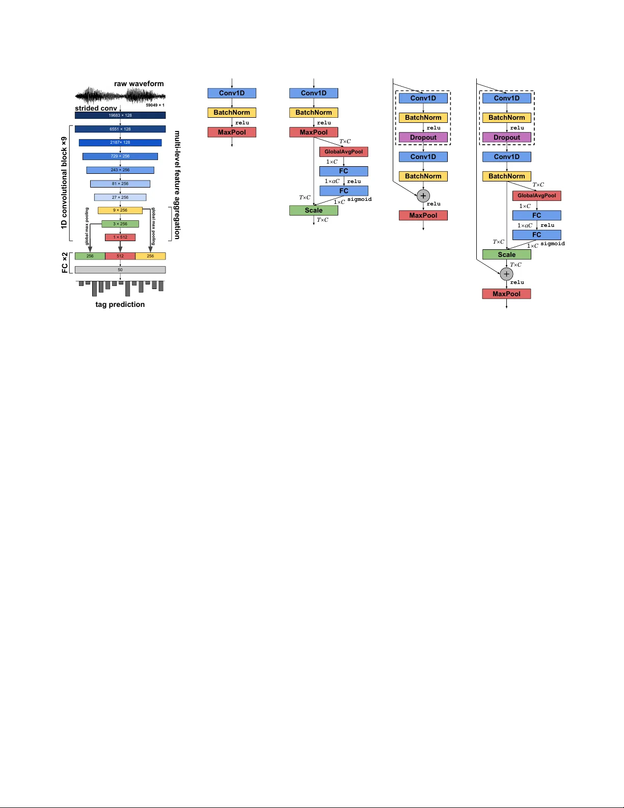
SAMPLE-LEVEL CNN ARCHITECTURES FOR MUSIC A UTO-T A GGING USING RA W W A VEFORMS T aejun Kim 1 , J ongpil Lee 2 , J uhan Nam 2 1 School of Electrical and Computer Engineering, Uni versity of Seoul, 2 Graduate School of Culture T echnology , KAIST , ktj7147@uos.ac.kr , { richter , juhannam } @kaist.ac.kr ABSTRA CT Recent work has sho wn that the end-to-end approach using con volutional neural network (CNN) is ef fective in v ari- ous types of machine learning tasks. For audio signals, the approach takes raw wa veforms as input using an 1-D con vo- lution layer . In this paper, we improve the 1-D CNN archi- tecture for music auto-tagging by adopting building blocks from state-of-the-art image classification models, ResNets and SENets , and adding multi-lev el feature aggre gation to it. W e compare different combinations of the modules in build- ing CNN architectures. The results sho w that they achie ve significant impro vements o ver previous state-of-the-art mod- els on the MagnaT agA T une dataset and comparable results on Million Song Dataset. Furthermore, we analyze and visualize our model to show ho w the 1-D CNN operates. Index T erms — con volutional neural networks, music auto-tagging, raw wa veforms, multi-lev el learning 1. INTR ODUCTION T ime-frequency representations based on short-time Fourier transform, often scaled in a log-like frequency such as mel- spectrogram, are the most common choice of input in the majority of state-of-the-art music classification algorithms [ 1 , 2 , 3 , 4 , 5 ]. The 2-dimentional input represents acousti- cally meaningful patterns well but requires a set of param- eters, such as window size/type and hop size, which may hav e different optimal settings depending on the type of input signals. In order to o vercome the problem, there ha ve been some efforts to directly use raw wa veforms as input particularly for con volutional neural networks (CNN) based models [ 6 , 7 ]. While they sho w promising results, the models used large fil- ters, expecting them to replace the Fourier transform. Re- cently , Lee et. al. [ 8 ] addressed the problem using v ery small filters and successfully applied the 1D CNN to the music auto- tagging task. Inspired from the well-known VGG net that uses very small size of filters such as 3 × 3 , [ 9 ], the sample-lev el CNN model was configured to take raw wav eforms as input and hav e filters with such small granularity . A number of techniques to further impro ve performances of CNNs ha ve appeared recently in image domain. He et. al. introduced ResNets which includes skip connections that en- ables a very deep CNN to be effecti vely trained and makes gradient propagation fluent [ 10 ]. Using the skip connections, they could successfully train a 1001-layer ResNet [ 11 ]. Hu et. al proposed SENets [ 12 ] which includes a b uilding block called Squeeze-and-Excitation (SE). Unlike other recent ap- proaches, the block concentrates on channel-wise informa- tion, not spatial. The SE block adaptively recalibrates feature maps using a channel-wise operation. Most of the techniques were dev eloped in the field of computer vision but they are not fully adopted for music classification tasks. Although there were a few approaches to readily apply them to audio domain [ 7 , 13 ]. They used 2D representations as input [ 13 ] or used large filters for the first 1D con volutional layer [ 7 ]. On the other hand, some methods are concerned with ov erall architecture of the model rather than designing a fine-grained building block [ 2 , 14 , 15 , 16 , 17 ]. Specifically , multi-lev el feature aggregation combines se veral hidden layer representations for final prediction [ 2 , 14 ]. They significantly improv ed the performance in music auto-tagging by taking different le vels of abstractions of tag labels into account. In this paper , we explore the b uilding blocks of ad- vanced CNN architectures, ResNets and SENets , based on the sample-lev el CNN for music auto-tagging. Also, we observe how the multi-level feature aggreg ation affects the performance. The results show that they achiev e significant improv ements ov er pre vious state-of-the-art models on the MagnaT agA T une dataset and comparable results on Million Song Dataset. Furthermore, we analyze and visualize our model b uilt with the SE blocks to sho w ho w the 1D CNN op- erates. The results show that the input signals are processed in a different manner depending on the le vel of layers. 2. ARCHITECTURES All of our models are based on the sample-lev el 1D CNN model [ 8 ], which is constructed with the basic block sho wn in Figure 1(b) . Every filter size of the con volution layers is fixed 6551 × 128 19683 × 128 2187× 128 729 × 256 243 × 256 81 × 256 27 × 256 9 × 256 3 × 256 256 512 256 1 × 512 50 tag prediction 1D convolutional block ×9 multi-level feature aggregation strided conv FC ×2 59049 × 1 raw waveform global max pooling global max pooling (a) Overvie w of the architecture Conv1D BatchNorm MaxPool relu (b) Basic block [ 8 ] relu relu sigmoid T×C 1 ×C 1 ×αC 1 ×C T×C T×C Conv1D FC FC Scale BatchNorm MaxPool GlobalAvgPool (c) SE block relu relu Conv1D BatchNorm Conv1D BatchNorm MaxPool Dropout (d) Res- n block relu relu sigmoid relu T×C 1 ×C 1 ×αC 1 ×C T×C T×C Conv1D BatchNorm Dropout Conv1D BatchNorm GlobalAvgPool FC FC Scale MaxPool (e) ReSE- n block Fig. 1 . The proposed architecture for music auto-tagging. (a) The models consist of a strided con volutional layer, 9 blocks, and two fully-connected (FC) layers. The outputs of the last three blocks are concatenated and then used as input of the last two FC layers. Output dimensions of each block (or layer) are denoted inside of them (temporal × channel). (b-e) The 1D con volutional building blocks that we e valuate. to three. The dif ferences between the sample-level CNN and ours are the use of adv anced building blocks and multi-le vel feature aggregation. In this section, we describe the details. 2.1. 1D con volutional building blocks 2.1.1. SE block W e utilize the SE block from SENets to increase representa- tional power of the basic block. As shown in Figure 1(c) , we simply attached the SE block to the basic block. The SE block recalibrates feature maps from the basic block through two operations. One is squeeze operation that aggreg ates a global temporal information into channel-wise statistics using global av erage pooling. The operation reduces the temporal dimen- sionality ( T ) to one, averaging outputs from each channel. The other is excitation operation that adapti vely recalibrates feature maps of each channel using the channel-wise statistics from the squeeze operation and a simple gating mechanism. The gating mechanism consists of two fully-connected (FC) layers that compute nonlinear interactions among channels. Finally , the original outputs from the basic block are rescaled by channel-wise multiplication between the feature map and the sigmoid activ ation of the second FC layer . Unlike the original SE block in SENets , our excitation op- eration does not form a bottleneck. On the contrary , we ex- pand the channel dimensionality ( C ) to αC at the first FC layer , and then reduce the dimensionality back to C at the second layer . W e set the amplifying ratio α to be 16, after a grid search with α = [2 − 3 , 2 − 2 , ..., 2 6 ] . 2.1.2. Res-n block Inspired by skip connections from ResNets , we modified the basic block by adding a skip connection as shown in Figure 1(d) . Res- n denotes that the block uses n conv olutional layers where n is one or two. Specifically , Res-2 is a block that has the additional layers denoted by the dotted line in Figure 1(d) , and Res-1 is a block that has a skip connection only . When the block uses two conv olutional layers ( Res-2 ), we add a dropout layer (with a drop ratio of 0.2) between two con volutions to avoid ov erfitting. This technique was firstly introduced at W ideResNets [ 18 ]. 2.1.3. ReSE-n block The ReSE- n block is a combination of the SE and Res- n blocks as sho wn in Figure 1(e) . n denotes the number of con- volutional layers in the block, where n is also one or two. A dropout layer is inserted when n is two. 2.2. Multi-level feature aggregation Fig. 1(a) shows the multi-level feature aggregations that we configured. The outputs of the last three blocks are concate- T able 1 . A UCs of CNN architectures on MT A T . “multi” and “no multi” indicates if the multi-lev el feature aggregation is used or not. † denotes using a weight decay of 10 − 4 . Block MT A T multi no multi Basic [ 8 ] 0.9077 0.9055 SE 0.9111 0.9083 Res-1 0.9037 0.9048 Res-2 0.9098 0.9061 ReSE-1 0.9053 0.9066 ReSE-2 0.9113 † 0.9102 † nated and then deliv ered to the FC layers. Before the con- catenation, temporal dimensions of the outputs are reduced to one by a global max pooling. Unlike [ 2 ], the concatenation occurs while training the CNN and the average pooling over the whole audio clip (i.e. 29 second long), which follo wed by the global max pooling, is not included. 3. EXPERIMENTS 3.1. Datasets W e ev aluated the proposed architectures on two datasets, MagnaT agA T une (MT A T) dataset [ 19 ] and Million Song Dataset (MSD) annotated with the Last.FM tags [ 20 ]. W e split and filtered both of the datasets, follo wing the previ- ous work [ 5 , 6 , 8 ]. W e used the 50 most frequent tags. All songs are trimmed to 29 seconds long, and resampled to 22050Hz as needed. The song is divided into 10 segments of 59049 samples. T o ev aluate the performance of music auto- tagging which is a multi-class and multi-label classification task, we computed the Area Under the Receiv er Operating Characteristic curve (A UC) for each tag and computed the av erage across all 50 tags. During the e valuation, we avera ge predictions across all segments. 3.2. Implementation details All the networks were trained using SGD with Nesterov mo- mentum of 0.9 and mini-batch size 23. The initial learning rate is set to 0.01, decayed by a f actor of 5 when a validation loss is on a plateau. None of the re gularizations are used on MSD. A dropout layer of 0.5 was inserted before the last FC layer on MT A T . For all building blocks, we ev aluated either with or without the multi-lev el feature aggregation. Since the training for MSD takes much time longer than MT A T , we ex- plored the architectures mainly on MT A T , and then trained the two best models on MSD. Code and models built with T en- sorFlow and K eras are av ailable at the link 1 . 1 https://github.com/tae- jun/resemul T able 2 . A UCs of state-of-the-art models on MT A T and MSD. † denotes that the model used an ensemble of three. Model MT A T MSD Bag of multi-scaled features [ 3 ] 0.8980 - End-to-end [ 6 ] 0.8815 - T ransfer learning [ 4 ] 0.8800 - Persistent CNN [ 21 ] 0.9013 - T ime-Frequency CNN [ 22 ] 0.9007 - T imbre CNN [ 23 ] 0.8930 - 2D CNN [ 5 ] 0.8940 0.8510 CRNN [ 1 ] - 0.8620 Multi-lev el & multi-scale [ 2 ] 0.9017 † 0.8878 † SampleCNN multi-features [ 14 ] 0.9064 † 0.8842 SampleCNN [ 8 ] 0.9055 0.8812 SE [This work] 0.9111 0.8840 ReSE [This work] 0.9113 0.8847 4. RESUL TS AND DISCUSSION 4.1. Comparison of the architectur es T able 1 summarizes the ev aluation results of compared CNN architectures on the MT A T dataset. They show that the SE block is more ef fective than the Res- n blocks, increasing the performance of the basic block for all cases. In the Res- n block, only adding the skip connection to the basic block (Res-1) actually decreases the performance. The combination of the SE and the Res-2 improves it slightly more. Howe ver , a training time of the ReSE-2 is 1.8 times longer than the ba- sic block whereas the SE block only 1.08 times longer . Thus, if the training or prediction time of the models is important, the SE model will be preferred to the ReSE-2. The effect of the multi-le vel aggre gation is valid for the majority of the models. W e obtained two best results in T able 1 by using the multi-lev el aggregation. 4.2. Comparison with state-of-the-arts T able 2 compares previous state-of-the-art models in music auto-tagging with our best models, the SE block and ReSE- 2 block, each with multi-level aggregation. On the MT A T dataset, our best models outperform all the previous results. On MSD, they are not the best but are comparable to the second-tier . 5. ANAL YSIS OF EXCIT A TION T o lay the groundwork for understanding how 1D CNNs op- erate, we analyze the sigmoid acti v ations of e xcitations in the SE blocks at different le vels graphically and quantitativ ely . In this section, we observe how the SE blocks recalibrate chan- nels, depending on which level they exist. The blocks used for the analysis are from the SE model using the multi-lev el 1st block 5th (mid) block 9th (last) block Fig. 2 . V isualization of the sigmoid acti vations of excitations in the SE model. The channel inde x was sorted by the av erage of the activ ations. feature aggregation and the y were trained on MT A T . The acti- vations were e xtracted from its test set. The activ ations were av eraged over all segments separately for each tag. 5.1. Graphical analysis For this analysis, we chose three tags, classical , metal , and dance that are not similar to each other as shown in T able 3 . Figure 2 sho ws the av erage sigmoid activ ations in the SE blocks for the songs with the three tags. The dif ferent le vels of activ ations indicate that the SE blocks process input audio differently depending on the tag (or genre) of the music. That is, ev ery block in Figure 2 fires different patterns of activ a- tions for each tag at a specific channel. This trend is strongest at the first block (top), weakest at the mid block (middle), and becomes stronger again at the last block (bottom). This trend is somewhat dif ferent from what are observ ed in the image domain [ 12 ], where the exclusiv eness of average excitation for input with dif ferent labels are monotonically increasing along the layers. Specifically , the first block fires high activ ations for classical , low ones for dance , and ev en lower ones for metal for the majority of the channels. On the other hand, the activ ations of the last block vary depending on the tags. For example, the activ ations of metal are high at some channels but low at the others, which makes the activ a- tions noisy ev en though the y are sorted. W e can interpret this result as follows. The first block normalizes the loudness of the audios because the block fires high activ ations for classi- cal music, which tend to have small v olume, and low activ a- T able 3 . Co-occurrence matrix of the tags used in Figure 2 classical metal dance classical 704 0 1 metal 0 166 0 dance 1 0 153 1 2 3 4 5 6 7 8 9 block level 0.02 0.03 0.04 0.05 std Fig. 3 . Standard deviations (std) of the acti vations of excita- tions across all tags along each layer . tions for metal music, which tend to ha ve large v olume. Also, the middle block processes common features among them as they ha ve similar le vels of activ ations. Finally , the noisy ex- clusiv eness in the last block indicates that they effecti vely dis- criminate the music with different tags. 5.2. Quantitative analysis W e assure the exclusi veness trend by measuring standard de- viations of the acti vations across all tags at e very level. Figure 3 sho ws that the higher the standard de viation is, the more the block responses to the song differently according to its tag. The result sho ws that the standard de viation is highest at the first block, it drops and stays lo w up to the 5th block and then increases gradually until the last block. That is, the four lower blocks except the the bottom one (2 to 5) tend to handle gen- eral features whereas the four upper blocks (6 to 9) tend to progressiv ely more discriminative features. 6. CONCLUSION W e proposed 1D con volutional building blocks based on the previous w ork, the sample-level CNN , ResNets , and SENets . The ReSE block, which is a combination of the three mod- els, showed the best performance. Also, the multi-level fea- ture aggre gation sho wed impro vements on the majority of the building blocks. Through the e xperiments, we obtained state- of-the-art performance on the MT A T dataset and high-ranked results on MSD. In addition, we analyzed the activ ations of excitation in SE model to understand the effect. W ith this analysis, we could observe that the SE blocks process non- similar songs exclusiv ely and how the different le vels of the model process the songs in a different manner . 7. REFERENCES [1] Keunw oo Choi, Gy ¨ orgy Fazekas, Mark Sandler , and Kyungh yun Cho, “Conv olutional recurrent neural net- works for music classification, ” in ICASSP . IEEE, 2017, pp. 2392–2396. [2] Jongpil Lee and Juhan Nam, “Multi-level and multi- scale feature aggregation using pretrained con volutional neural networks for music auto-tagging, ” IEEE Signal Pr ocessing Letters , v ol. 24, no. 8, pp. 1208–1212, 2017. [3] Sander Dieleman and Benjamin Schrauwen, “Multi- scale approaches to music audio feature learning, ” in In- ternational Society of Music Information Retrieval Con- fer ence (ISMIR) , 2013, pp. 116–121. [4] A ¨ aron V an Den Oord, Sander Dieleman, and Ben- jamin Schrauwen, “Transfer learning by supervised pre- training for audio-based music classification, ” in Inter - national Society of Music Information Retrieval Confer- ence (ISMIR) , 2014. [5] Keunw oo Choi, Gy ¨ orgy Fazekas, and Mark B. Sandler, “ Automatic tagging using deep con volutional neural net- works, ” in International Society of Music Information Retrieval Conference (ISMIR) , 2016. [6] Sander Dieleman and Benjamin Schrauwen, “End-to- end learning for music audio, ” in ICASSP . IEEE, 2014, pp. 6964–6968. [7] W ei Dai, Chia Dai, Shuhui Qu, Juncheng Li, and Samar- jit Das, “V ery deep con volutional neural networks for raw wa veforms, ” in ICASSP . IEEE, 2017, pp. 421–425. [8] Jongpil Lee, Jiyoung P ark, Keunh young Luke Kim, and Juhan Nam, “Sample-lev el deep con volutional neu- ral networks for music auto-tagging using ra w wa ve- forms, ” in Sound and Music Computing Conference (SMC) , 2017. [9] Karen Simonyan and Andre w Zisserman, “V ery deep con volutional networks for large-scale image recogni- tion, ” ICLR , 2015. [10] Kaiming He, Xiangyu Zhang, Shaoqing Ren, and Jian Sun, “Deep residual learning for image recognition, ” in IEEE Conference on Computer V ision and P attern Recognition (CVPR) , 2016, pp. 770–778. [11] Kaiming He, Xiangyu Zhang, Shaoqing Ren, and Jian Sun, “Identity mappings in deep residual networks, ” in European Confer ence on Computer V ision (ECCV) . Springer , 2016, pp. 630–645. [12] Jie Hu, Li Shen, and Gang Sun, “Squeeze-and- excitation netw orks, ” arXiv pr eprint arXiv:1709.01507 , 2017. [13] Shawn Hershey , Sourish Chaudhuri, Daniel P . W . El- lis, Jort F . Gemmeke, Aren Jansen, R. Channing Moore, Manoj Plakal, Devin Platt, Rif A. Saurous, Bryan Sey- bold, Malcolm Slaney , Ron J. W eiss, and Ke vin W . W il- son, “Cnn architectures for lar ge-scale audio classifica- tion, ” in ICASSP . IEEE, 2017, pp. 131–135. [14] Jongpil Lee and Juhan Nam, “Multi-level and multi- scale feature aggregation using sample-lev el deep con- volutional neural networks for music classification, ” Machine Learning for Music Discovery W orkshop, In- ternational Confer ence on Machine Learning (ICML) , 2017. [15] Y i Sun, Xiaogang W ang, and Xiaoou T ang, “Deep learn- ing face representation from predicting 10,000 classes, ” in IEEE Conference on Computer V ision and P attern Recognition (CVPR) , 2014, pp. 1891–1898. [16] Jeff Donahue, Y angqing Jia, Oriol V inyals, Judy Hoff- man, Ning Zhang, Eric Tzeng, and T rev or Darrell, “De- caf: A deep con volutional activ ation feature for generic visual recognition, ” in International Confer ence on Ma- chine Learning (ICML) , 2014, pp. 647–655. [17] Y usuf A ytar , Carl V ondrick, and Antonio T orralba, “Soundnet: Learning sound representations from unla- beled video, ” in Neural Information Pr ocessing Systems (NIPS) , 2016, pp. 892–900. [18] Serge y Zagoruyko and Nikos Komodakis, “Wide resid- ual networks, ” British Machine V ision Confer ence (BMVC) , 2016. [19] Edith Law , Kris W est, Michael I. Mandel, Mert Bay , and J. Stephen Downie, “Evaluation of algorithms us- ing games: The case of music tagging, ” in International Society of Music Information Retrie val Confer ence (IS- MIR) , 2009. [20] Thierry Bertin-Mahieux, Daniel P . W . Ellis, Brian Whit- man, and Paul Lamere, “The million song dataset, ” in International Society of Music Information Retrieval Confer ence (ISMIR) , 2011, vol. 2, p. 10. [21] Jen-Y u Liu, Shyh-Kang Jeng, and Y i-Hsuan Y ang, “ Ap- plying topological persistence in con volutional neu- ral network for music audio signals, ” arXiv preprint arXiv:1608.07373 , 2016. [22] Umut G ¨ uc ¸ l ¨ u, Jordy Thielen, Michael Hanke, Marcel van Gerven, and Marcel AJ van Gerven, “Brains on beats, ” in Neural Information Pr ocessing Systems (NIPS) , 2016, pp. 2101–2109. [23] Jordi Pons, Olga Slizovskaia, Rong Gong, Emilia G ´ omez, and Xavier Serra, “T imbre analysis of music au- dio signals with con volutional neural networks, ” arXiv pr eprint arXiv:1703.06697 , 2017.