Iterative Sparse Asymptotic Minimum Variance Based Approaches for Array Processing

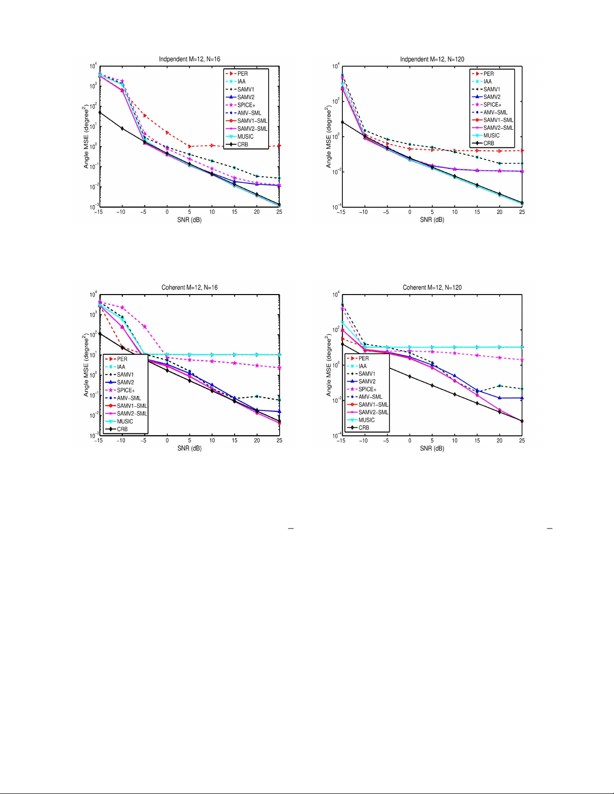
1 Iterativ e Sparse Asymptotic Minimum V ariance Based A ppr oaches f or Array Pr ocessing Habti Abeida ∗ , Qilin Zhang † , Jian Li ‡ and Nadjim Merabtine § ∗ Department of Electrical Engineering, Uni versity of T aif, Al-Haweiah, Saudi Arabia † Department of Computer Science, Ste vens Institue of T echnology , Hobok en, NJ, USA ‡ Department of Electrical and Computer Engineering, Uni versity of Florida, Gainesville, FL, USA § Department of Electrical Engineering, Uni versity of T aif, Al-Haweiah, Saudi Arabia Abstract This paper presents a series of user parameter-free iterativ e Sparse Asymptotic Minimum V ariance (SAMV) approaches for array processing applications based on the asymptotically minimum variance (AMV) criterion. W ith the assumption of abundant snapshots in the direction-of-arriv al (DOA) estimation problem, the signal powers and noise v ariance are jointly estimated by the proposed iterati ve AMV approach, which is later proved to coincide with the Maximum Likelihood (ML) estimator . W e then propose a series of power -based iterativ e SAMV approaches, which are rob ust against insufficient snapshots, coherent sources and arbitrary array geometries. Moreov er , to over - come the direction grid limitation on the estimation accuracy , the SAMV -Stochastic ML (SAMV -SML) approaches are deriv ed by explicitly minimizing a closed form stochastic ML cost function with respect to one scalar parameter, eliminating the need of any additional grid refinement techniques. T o assist the performance ev aluation, approximate solutions to the SAMV approaches are also provided at high signal-to-noise ratio (SNR) and low SNR, respectiv ely . Finally , numerical examples are generated to compare the performance of the proposed approaches with existing approaches. Index terms: Array Processing, AMV estimator, Direction-Of-Arriv al (DO A) estimation, Sparse parameter estima- tion, Covariance matrix, Iterativ e methods, V ectors, Arrays, Maximum likelihood estimation, Signal to noise ratio, SAMV approach. Preprint version PDF av ailable on arXi v . Official version: Abeida Habti, Qilin Zhang, Jian Li, and Nadjim Merabtine . “Iterative sparse asymptotic minimum variance based appr oaches for array pr ocessing. ” IEEE T r ansactions on Signal Pr ocessing 61, no. 4 (2013): 933-944. Matlab implementation codes av ailable online, https://qilin- zhang.github .io/publications/ I . I N T RO D U C T I O N Sparse signal representation has attracted a lot of attention in recent years and it has been successfully used for solving in verse problems in various applications such as channel equalization (e.g., [7], [8], [9], [10]), source localization (e.g., [15], [16], [35], [34]) and radar imaging (e.g., [11], [12], [13], [14]). In its basic form, it attempts to find the sparsest signal x satisfying the constrain y = Ax or y = Ax + e where A ∈ C M × K is an overcomplete basis (i.e., K > M ), y is the observ ation data, and e is the noise term. Theoretically , this problem is underdetermined and has multiple solutions. Ho wev er, the additional constraint that x should be sparse allo ws one to eliminate the ill-posedness (e.g., [1], [2]). In recent years, a number of practical algorithms such as ` 1 norm minimization (e.g., [3], [4]) and focal underdetermined system solution (FOCUSS) (e.g., [5], [6]) have been proposed to approximate the sparse solution. Con ventional subspace-based source localization algorithms such as multiple signal classification (MUSIC) and estimation of signal parameters via a rotational in variance technique (ESPRIT) [17], [18] are only applicable when M > K , and the y require sufficient snapshots and high signal-to-noise ratio (SNR) to achiev e high spatial resolution. Ho wever , it is often unpractical to collect a large number of snapshots, especially in fast time-varying en vironment, which deteriorates the construction accuracy of the subspaces and de grades the localization performance. In addition, e ven with appropriate array calibration, subspace-based methods are incapable of handling the source coherence due to their sensitivity to subspace orthogonality (e.g., [17], [19]). 2 Recently , a user parameter-free non-parametric algorithm, the iterative adaptiv e approach (IAA), has been pro- posed in [16] and employed in various applications (e.g., [12], [13]). It is demonstrated in these works that the least square fitting-based IAA algorithm provides accurate DO A and signal po wer estimates, and it is insensitiv e to practical impairments such as fe w (ev en one) snapshots, arbitrary array geometries and coherent sources. Howe ver , the iterativ e steps are based on the IAA covariance matrix R = A Diag ( p ) A H , which could be singular in the noise- free scenarios when only a few components of the po wer vector p are non-zero. In addition, a regularized version of the IAA algorithm (IAA-R) is later proposed in [13] for single-snapshot and nonuniform white noise cases. Stoica et al. ha ve recently proposed a user parameter-free SParse Iterative Covariance-based Estimation (SPICE) approach in [20], [21] based on minimizing a covariance matrix fitting criterion. Howe ver , the SPICE approach proposed in [20] for the multiple-snapshot case depends on the in verse of the sample cov ariance matrix, which exists only if the number of snapshot N is lar ger than M [31]. Therefore, this approach also suffers from insuf ficient snapshots when N < M . W e note that the source localization performance of the po wer-based algorithms is mostly limited by the fineness of the direction grid [15]. In this paper , we propose a series of iterati ve Sparse Asymptotic Minimum V ariance (SAMV) approaches based on the asymptotically minimum variance (AMV) approach (also called asymptotically best consistent (ABC) estimators in [23]), which is initially proposed for DO A estimation in [28], [27]. After presenting the sparse signal representation data model for the DOA estimation problem in Section II, we first propose an iterativ e AMV approach in Section III, which is later proven to be identical to the stochastic Maximum Likelihood (ML) estimator . Based on this approach, we then propose the user parameter-free iterativ e SAMV approaches that can handle arbitrary number of snapshots ( N < M or N > M ), and only a few non-zero components in the power estimates vector p in Section IV. In addition, A series of SAMV -Stochastic ML (SAMV -SML) approaches are proposed in Section V to alleviate the direction grid limitation and enhance the performance of the power-based SAMV approaches. In Section VI, we deriv e approximate expressions for the SAMV powers-iteration formulas at both high and low SNR. In Section VII, numerical examples are generated to compare the performances of the proposed approaches with existing approaches. Finally , conclusions are giv en in Section VIII. The following notations are used throughout the paper . Matrices and vectors are represented by bold upper case and bold lower case characters, respectiv ely . V ectors are by default in column orientation, while T , H , and ∗ stand for transpose, conjugate transpose, and conjugate, respectively . E( · ) , T r( · ) and det( · ) are the expectation, trace and determinant operators, respecti vely . v ec( · ) is the “vectorization” operator that turns a matrix into a vector by stacking all columns on top of one another, ⊗ denotes the Kronecker product, I is the identity matrix of appropriate dimension, and e m denotes the m th column of I . I I . P R O B L E M F O R M A T I O N A N D D A TA M O D E L Consider an array of M omnidirectional sensors receiving K narro wband signals impinging from the sources located at θ def = ( θ 1 , . . . , θ K ) where θ k denotes the location parameter of the k th signal, k = 1 , . . . , K . The M × 1 array snapshot vectors can be modeled as (see e.g., [16], [20]) y ( n ) = Ax ( n ) + e ( n ) , n = 1 , . . . , N , (1) where A def = [ a ( θ 1 ) , . . . , a ( θ K )] is the steering matrix with each column being a steering vector a k def = a ( θ k ) , a kno wn function of θ k . The vector x ( n ) def = [ x 1 ( n ) , . . . , x K ( n )] T contains the source wav eforms, and e ( n ) is the noise term. Assume that E  e ( n ) e H ( ¯ n )  = σ I M δ n, ¯ n 1 , where δ n, ¯ n is the Dirac delta and it equals to 1 only if n = ¯ n and 0 otherwise. W e also assume first that e ( n ) and x ( n ) are independent, and that E  x ( n ) x H ( ¯ n )  = P δ n, ¯ n , where P def = Diag( p 1 , . . . , p K ) . Let p be a vector containing the unknown signal powers and noise variance, p def = [ p 1 , . . . , p K , σ ] T . The cov ariance matrix of y ( n ) that con ve ys information about p is gi ven by R def = AP A H + σ I . This cov ariance matrix is traditionally estimated by the sample cov ariance matrix R N def = YY H / N where Y def = [ y (1) , . . . , y ( N )] . After applying the vectorization operator to the matrix R , the obtained vector r ( p ) def = vec( R ) 1 The nonuniform white noise case is considered later in Remark 2. 3 is linearly related to the unknown parameter p as r ( p ) def = vec( R ) = Sp , (2) where S def = [ S 1 , ¯ a K +1 ] , S 1 = [ ¯ a 1 , . . . , ¯ a K ] , ¯ a k def = a ∗ k ⊗ a k , k = 1 , . . . K , and ¯ a K +1 def = vec( I ) . W e note that the Gaussian circular asymptotic cov ariance matrix r N def = vec( R N ) is giv en by [29, Appendix B], [28] C r = R ∗ ⊗ R . The number of sources, K , is usually unknown. The power -based algorithms, such as the proposed SAMV approaches, use a predefined scanning direction grid { θ k } K k =1 to cover the entire region-of-interest Ω , and ev ery point in this grid is considered as a potential source whose po wer is to be estimated. Consequently , K is the number of points in the grid and it is usually much larger than the actual number of sources present, and only a few components of p will be non-zero. This is the main reason why sparse algorithms can be used in array processing applications [20], [21]. T o estimate the parameter p from the statistic r N , we develop a series of iterative SAMV approaches based on the AMV approach introduced by Porat and Fridelander in [22], Stoica et al. in [23] with their asymptotically best consistent (ABC) estimator , and Delmas and Abeida in [28], [27]. I I I . T H E A S Y M P T O T I C A L LY M I N I M U M V A R I A N C E A P P R O AC H In this section, we dev elop a recursi ve approach to estimate the signal powers and noise variance (i.e., p ) based on the AMV criterion using the statistic r N . W e assume that p is identifiable from r ( p ) . Exploiting the similarities to the works in [28], [27], it is straightforward to prove that the cov ariance matrix Cov Alg p of an arbitrary consistent estimator of p based on the second-order statistic r N is bounded below by the following real symmetric positiv e definite matrix: Co v Alg p ≥ [ S H d C − 1 r S d ] − 1 , where S d def = d r ( p ) / d p . In addition, this lo wer bound is attained by the cov ariance matrix of the asymptotic distribution of ˆ p obtained by minimizing the following AMV criterion: ˆ p = arg min p f ( p ) , where f ( p ) def = [ r N − r ( p )] H C − 1 r [ r N − r ( p )] . (3) From (3) and using (2), the estimate of p is gi ven by the following results proved in Appendix A: Result 1. The { ˆ p k } K k =1 and ˆ σ that minimize (3) can be computed iteratively . Assume ˆ p ( i ) k and ˆ σ ( i ) have been obtained in the i th iteration, the y can be updated at the ( i + 1) th iteration as: ˆ p ( i +1) k = a H k R − 1( i ) R N R − 1( i ) a k ( a H k R − 1( i ) a k ) 2 + ˆ p ( i ) k − 1 a H k R − 1( i ) a k , k = 1 . . . , K , (4) ˆ σ ( i +1) =  T r( R − 2 ( i ) R N ) + ˆ σ ( i ) T r( R − 2 ( i ) ) − T r( R − 1 ( i ) )  / T r( R − 2 ( i ) ) , (5) wher e the estimate of R at the i th iteration is given by R ( i ) = AP ( i ) A H + ˆ σ ( i ) I with P ( i ) = Diag( ˆ p ( i ) 1 , . . . , ˆ p ( i ) K ) . Assume that x ( n ) and e ( n ) are both circularly Gaussian distributed, y ( n ) also has a circular Gaussian distribution with zero-mean and cov ariance matrix R . The stochastic negativ e log-likelihood function of { y ( n ) } N n =1 can be expressed as (see, e.g., [26], [16]) L ( p ) = ln(det( R )) + T r( R − 1 R N ) . (6) In lieu of the cost function (3) that depends linearly on p (see (2)), this ML cost-function (6) depends non-linearly on the signal powers and noise variance embedded in R . Despite this dif ficulty and reminiscent of [16], we prove in Appendix B that the following result holds: 4 Result 2. The estimates given by (4) and (5) ar e identical to the ML estimates. Consequently , there always exists approaches that giv es the same performance as the ML estimator which is asymptotically efficient. Returning to the Result 1, first we notice that the expression given by (4) remains v alid regardless of K > M or K < M . In the scenario where K > M , we observe from numerical calculations that the ˆ p k and ˆ σ gi ven by (4) and (5) may be neg ative; therefore, the nonnegati vity of the power estimates can be enforced at each iteration by forcing the negati ve estimates to zero as [16, Eq. (30)], ˆ p ( i +1) k = max 0 , a H k R − 1( i ) R N R − 1( i ) a k ( a H k R − 1( i ) a k ) 2 + ˆ p ( i ) k − 1 a H k R − 1( i ) a k ! , k = 1 . . . , K , (7) ˆ σ ( i +1) = max  0 ,  T r( R − 2 ( i ) R N ) + ˆ σ ( i ) T r( R − 2 ( i ) ) − T r( R − 1 ( i ) )  / T r( R − 2 ( i ) )  . The above updating formulas of ˆ p k and ˆ σ at ( i + 1) th iteration require knowledge of R , ˆ p k and ˆ σ at the i th iteration, hence this algorithm must be implemented iterativ ely . The initialization of ˆ p k can be done with the periodogram (PER) po wer estimates (see, e.g., [30]) ˆ p (0) k, PER = a H k R N a k k a k k 4 . (8) The noise v ariance estimator ˆ σ can be initialized as, for instance, ˆ σ = 1 M N N X n =1 k y ( n ) k 2 . (9) Remark 1. In the classical scenario wher e ther e are mor e sensors than sour ces (i.e., K ≤ M ), closed form appr oximate ML estimates of a single sour ce power and noise variance ar e derived in [25] and [24] assuming uniform white noise and nonuniform white noise, r espectively . However , these appr oximate expr essions are derived at high and low SNR re gimes separately 2 , compar ed to the unified e xpressions (4) and (5) re gar dless of SNR or number of sour ces. Remark 2. Result 1 can be extended easily to the nonuniform white Gaussian noise case wher e the covariance matrix is given by E  e ( n ) e H ( n )  = Diag( σ 1 , . . . , σ M ) def = M X m =1 σ m a K + m a T K + m , (10) wher e a K + m def = e m , m = 1 , . . . , M , denote the canonical vectors. Under these assumptions and fr om Result 1, the estimates of p at ( i + 1) th iteration ar e given by ˆ p ( i +1) k = a H k R − 1( i ) R N R − 1( i ) a k ( a H k R − 1( i ) a k ) 2 + ˆ p ( i ) k − 1 a H k R − 1( i ) a k , k = 1 . . . , K + M , (11) wher e R ( i ) = AP ( i ) A H + P M m =1 ˆ σ ( i ) m a K + m a T K + m , P ( i ) = Diag( ˆ p ( i ) 1 , . . . , ˆ p ( i ) K ) and ˆ σ ( i ) m = ˆ p ( i ) K + m , m = 1 , . . . , M . As mentioned before, the ˆ p k may be negati ve when K > M , therefore, the po wer estimates can be iterated similar to (7) by forcing the negati ve values to zero. I V . T H E S PA R S E A S Y M P T O T I C M I N I M U M V A R I A N C E A P P R O AC H E S In this section, we propose the iterative SAMV approaches to estimate p ev en when K exceeds the number of sources K (i.e., when the steering matrix A can be viewed as an ov ercomplete basis for y ( n ) ) and only a few non-zero components are present in p . This is the common case encountered in many spectral analysis applications, where only the estimation of p is deemed rele vant (e.g., [20], [21]). As mentioned in Result 2, the estimates given by (4) and (5) may gi ve irrational negati ve v alues due to the presence of the non-zero terms p k − 1 / ( a H k R − 1 a k ) and σ − T r( R − 1 ) / T r( R − 2 ) . T o resolve this difficulty , we assume that 3 2 For high and low SNR, the ML function (6) is linearized by different approximations in [25] and [24] 3 p k = 1 / ( a H k R − 1 a k ) is the standard Capon power estimate [30]. 5 p k = 1 / ( a H k R − 1 a k ) and σ = T r( R − 1 ) / T r( R − 2 ) , and propose the following SAMV approaches based on Result 1: SAMV -0 appr oach: The estimates of p k and σ are updated at ( i + 1) th iteration as: ˆ p ( i +1) k = ˆ p 2( i ) k ( a H k R − 1( i ) R N R − 1( i ) a k ) , k = 1 , . . . , K , (12) ˆ σ ( i +1) = T r( R − 2( i ) R N ) T r( R − 2( i ) ) . (13) SAMV -1 appr oach: The estimates of p k and σ are updated at ( i + 1) th iteration as: ˆ p ( i +1) k = a H k R − 1( i ) R N R − 1( i ) a k ( a H k R − 1( i ) a k ) 2 , k = 1 , . . . , K , (14) ˆ σ ( i +1) = T r( R − 2( i ) R N ) T r( R − 2( i ) ) . (15) SAMV -2 appr oach: The estimates of p k and σ are updated at ( i + 1) th iteration as: ˆ p ( i +1) k = ˆ p ( i ) k a H k R − 1( i ) R N R − 1( i ) a k a H k R − 1( i ) a k , k = 1 , . . . , K , (16) ˆ σ ( i +1) = T r( R − 2( i ) R N ) T r( R − 2( i ) ) . In the case of nonuniform white Gaussian noise with covariance matrix giv en in Remark 2, the SAMV noise po wers estimates can be updated alternati vely as ˆ σ ( i +1) m = e H m R − 1( i ) R N R − 1( i ) e m ( e H m R − 1( i ) e m ) 2 , m = 1 . . . , M , (17) where R ( i ) = AP ( i ) A H + P M m =1 ˆ σ ( i ) m e m e T m , P ( i ) = Diag( ˆ p ( i ) 1 , . . . , ˆ p ( i ) K ) and e m are the canonical vectors, m = 1 , . . . , M . In the following Result 3 prov ed in Appendix C, we show that the SAMV -1 signal po wer and noise variance updating formulas giv en by (14) and (15) can also be obtained by minimizing a weighted least square (WLS) cost function. Result 3. The SAMV -1 estimate is also the minimizer of the following WLS cost function: ˆ p k = arg min p k g ( p k ) , wher e g ( p k ) def = arg min p k [ r N − p k ¯ a k ] H C 0− 1 k [ r N − p k ¯ a k ] . (18) and C 0 k def = C r − p 2 k ¯ a k ¯ a H k , k = 1 , . . . , K + 1 . The implementation steps of the these SAMV approaches are summarized in T able 1. T ABLE 1 The SAMV approaches Initialization: { p (0) k } K k =1 and ˆ σ (0) using e.g., (8) and (9). repeat • Update R ( i ) = AP ( i ) A H + σ ( i ) I , • Update ˆ p ( i +1) k using SAMV formulas (12) or (14) or (16), • Update ˆ σ ( i +1) using (15). 6 Remark 3. Since R N = 1 N P N n =1 y ( n ) y H ( n ) , the SAMV -1 sour ce power updating formula (14) becomes p ( i +1) k = 1 N ( a H k R − 1( i ) a k ) 2 N X n =1 | a H k R − 1( i ) y ( n ) | 2 . (19) Comparing this e xpression with its IAA counterpart ([16, T able II]), we can see that the differ ence is that the IAA power estimate is obtained by adding up the signal magnitude estimates { x k ( n ) } N n =1 . The matrix R in the IAA appr oach is obtained as AP A H , wher e P = Diag ( p 1 , . . . , p K ) . This R can suffer fr om matrix singularity when only a few elements of { p k } K k =1 ar e non-zer o (i.e., the noise-fr ee case). Remark 4. W e note that the SPICE+ algorithm derived in [20] for the multiple snapshots case r equir es that the matrix R N be nonsingular , which is true with pr obability 1 if N ≥ M [31]. This implies that this algorithm can not be applied when N < M . On contr ary , this condition is not requir ed for the pr oposed SAMV appr oaches, which do not depend on the in verse of R N . In addition, these SAMV appr oaches pr ovide good spatial estimates even with a few snapshots, as is shown in section VII. V . D O A E S T I M A T I O N : T H E S PA R S E A S Y M P T O T I C M I N I M U M V A R I A N C E - S T O C H A S T I C M A X I M U M L I K E L I H O O D A P P RO A C H E S It has been noticed in [15] that the resolution of most po wer-based sparse source localization techniques is limited by the fineness of the direction grid that cov ers the location parameter space. In the sparse signal recov ery model, the sparsity of the truth is actually dependent on the distance between the adjacent element in the ov ercomplete dictionary , therefore, the dif ficulty of choosing the optimum overcomplete dictionary (i.e., particularly , the DO A scanning direction grid) arises. Since the computational complexity is proportional to the fineness of the direction grid, a highly dense grid is not computational practical. T o o vercome this resolution limitation imposed by the grid, we propose the grid-free SAMV -SML approaches, which refine the location estimates θ = ( θ 1 , . . . , θ K ) T by iterati vely minimizing a stochastic ML cost function with respect to a single scalar parameter θ k . Using (47), the ML objectiv e function can be decomposed into L ( θ − k ) , the marginal likelihood function with parameter θ k excluded, and l ( θ k ) with terms concerning θ k : l ( θ k ) def = ln  1 1 + p k α 1 ,k  + p k α N 2 ,k 1 + p k α 1 ,k , (20) where the α 1 ,k and α N 2 ,k are defined in Appendix B. Therefore, assuming that the parameter { p k } K k =1 and σ are estimated using the SAMV approaches 4 , the estimate of θ k can be obtained by minimizing (20) with respect to the scalar parameter θ k . The classical stochastic ML estimates are obtained by minimizing the cost function with respect to a multi- dimensional vector { θ k } K k =1 , (see e.g., [26, Appendix B, Eq. (B.1)]). The computational complexity of the multi- dimensional optimization is so high that the classical stochastic ML estimation problem is usually unsolv able. On contrary , the proposed SAMV -SML algorithms only require minimizing (20) with respect to a scalar θ k , which can be ef ficiently implemented using deriv ati ve-free uphill search methods such as the Nelder-Mead algorithm 5 [33]. The SAMV -SML approaches are summarized in T able 2. T ABLE 2 The SAMV -SML approaches Initialization: { p (0) k } K k =1 , ˆ σ (0) and { ˆ θ (0) k } K k =1 based on the result of SAMV approaches, e.g., SAMV -3 estimates, (16) and (15). repeat • Compute R ( i ) and Q ( i ) k gi ven by (43), • Update p k using (4) or (14) or (16), update σ using (5) or (15), • Minimizing (20) with respect to θ k to obtain the stochastic ML estimates ˆ θ k . 4 SAMV -SML variants use different p k and σ estimates: AMV -SML: (4) and (5), SAMV1-SML: (14) and (15), SAMV2-SML: (16) and (15). 5 The Nelder-Mead algorithm has already been incorporated in the function “fminsearch” in MA TLAB R  . 7 V I . H I G H A N D L O W S N R A P P R OX I M AT I O N T o get more insights into the SAMV approaches, we deriv e the following approximate expressions for the SAMV approaches at high and low SNR, respectiv ely . 1) Zer o-Or der Low SNR Appr oximation: Note that the in verse of the matrix R can be written as: R − 1 =  ¯ R + σ I  − 1 = ¯ R − 1 − ¯ R − 1  1 σ I + ¯ R − 1  − 1 ¯ R − 1 , where ¯ R def = AP A H . (21) At lo w SNR (i.e., p k σ  1 ), from (21), we obtain R − 1 ≈ 1 σ I . Thus, a H k R − 1 R N R − 1 a k ≈ 1 σ 2 ( a H k R N a k ) , (22) a H k R − 1 a k ≈ M 2 σ , (23) T r( R − 2 R N ) ≈ 1 N σ 2 N X n =1 k y ( n ) k 2 , (24) T r( R − 2( i ) ) ≈ M σ 2 . (25) Substituting (22) and (23) into the SAMV updating formulas (12)-(16), we obtain ˆ p ( i +1) k, SAMV − 0 = M 2 ˆ σ 2 ˆ p 2( i ) k, SAMV − 0 ˆ p k, PER , (26) ˆ p k, SAMV − 1 = ˆ p k, PER , (27) ˆ p ( i +1) k, SAMV − 2 = M ˆ σ ˆ p ( i ) k, SAMV − 2 ˆ p k, PER , (28) where ˆ p k, PER is gi ven by (8). Using (24) and (25), the common SAMV noise updating equation (15) is approximated as ˆ σ = 1 M N N X n =1 k y ( n ) k 2 . From (27), we comment that the SAMV -1 approach is equi valent to the PER method at lo w SNR. In addition, we remark that at very low SNR, the SAMV -0 and SAMV -2 power estimates gi ven by (26) and (28) are scaled versions of the PER estimate ˆ p k, PER , provided that they are both initialized by PER. 2) Zer o-Or der High SNR Appr oximation: At high SNR (i.e., p k σ  1 ), from (21), we obtain R − 1 ≈ ¯ R − 1 . Thus, a H k R − 1 R N R − 1 a k ≈ a H k ¯ R − 1 R N ¯ R − 1 a k , (29) a H k R − 1 a k ≈ a H k ¯ R − 1 a k . (30) Substituting (29) and (30) into the SAMV formulas (12)–(16) yields: p ( i +1) k, SAMV − 0 = p 2( i ) k, SAMV − 0 ( a H k ¯ R − 1( i ) R N ¯ R − 1( i ) a k ) , (31) p ( i +1) k, SAMV − 1 = a H k ¯ R − 1( i ) R N ¯ R − 1( i ) a k ( a H k ¯ R − 1( i ) a k ) 2 , (32) p ( i +1) k, SAMV − 2 = p ( i ) k, SAMV − 2 a H k ¯ R − 1( i ) R N ¯ R − 1( i ) a k a H k ¯ R − 1( i ) a k . (33) From (32), we get p ( i +1) k = a H k ¯ R − 1( i ) R N ¯ R − 1( i ) a k ( a H k ¯ R − 1( i ) a k ) 2 = 1 N N X n =1 | x ( i ) k, IAA ( n ) | 2 , (34) where x ( i ) k, IAA ( n ) def = a H k ¯ R − 1( i ) y ( n ) a H k ¯ R − 1( i ) a k is the the signal wa veform estimate at the direction θ k and n th snapshot[16, Eq. (7)]. From (34), we comment that SAMV -1 and IAA are equi valent at high SNR. The only difference is that the IAA po wers estimates are obtained by summing up the signal magnitude estimates { x k, IAA ( n ) } N n =1 . 8 V I I . S I M U L A T I O N R E S U LT S A. Source Localization This subsection focuses on e valuating the performances of the proposed SAMV and SAMV -SML algorithms using an M = 12 element uniform linear array (ULA) with half-wav elength inter-element spacing, since the application of the proposed algorithms to arbitrary arrays is straightforward. For all the considered po wer-based approaches, the scanning direction grid { θ k } K k =1 is chosen to uniformly cov er the entire region-of-interest Ω = [0 ◦ 180 ◦ ) with the step size of 0 . 2 ◦ . The v arious SNR values are achieved by adjusting the noise v ariance σ , and the SNR is defined as: SNR , 10 log 10  p avg σ  [ dB ] , (35) where p avg denotes the a verage po wer of all sources. For K sources, p avg , 1 K P K k =1 p k . First, DO A estimation results using a 12 element ULA and N = 120 snapshots of both independent and coherent sources are gi ven in Figure 1 and Figure 2, respectiv ely . Three sources with 5 dB, 3 dB and 4 dB po wer at location θ 1 = 35 . 11 ◦ , θ 2 = 50 . 15 ◦ and θ 3 = 55 . 05 ◦ are present in the region-of-interest. For the coherent sources case in Figure 2, the sources at θ 1 and θ 3 share the same phases but the source at θ 2 are independent of them. The true source locations and powers are represented by the circles and vertical dashed lines that align with these circles. In each plot, the estimation results of 10 Monte Carlo trials for each algorithm are shown together . Due to the strong smearing ef fects and limited resolution, the PER approach fails to correctly separate the close sources at θ 2 and θ 3 (Figure 1(a) and Figure 2(a)). The IAA algorithm has reduced the smearing ef fects significantly , resulting lo wer sidelobe lev els in Figure 1(b) and Figure 2(b). Ho wever , the resolution provided by IAA is still not high enough to separate the two close sources at θ 2 and θ 3 . In the scenario with independent sources, the eigen-analysis based MUSIC algorithm and existing sparse methods such as the SPICE+ algorithm, are capable of resolving all three sources in Figure 1(c)–(d), thanks to their superior resolution. Howe ver , the source coherence degrades their performances dramatically in Figure 2(c)–(d). On contrary , the proposed SAMV algorithms depicted in Figure 2(e)–(g), are much more robust against signal coherence. W e observe in Figure 1 – 2 that the SAMV -1 approach generally provides identical spatial estimates to its IAA counterpart and this phenomenon is again revealed in Figure 3 – 4, which verifies the comments in Section VI. In Figure 1 – 2, the SAMV -0 and SAMV -2 algorithm generate high resolution sparse spatial estimates for both the independent and coherent sources. Ho wev er, we notice in our simulations that the sparsest SAMV -0 algorithm requires a high SNR to work properly . Therefore, SAMV -0 is not included when comparing angle estimation mean-square-error ov er a wide range of SNR in Figure 3 – 4. From Figure 1 – 2, we comment that the SAMV -SML algorithms (AMV - SML, SAMV1-SML and SAMV2-SML) provide the most accurate estimates of the source locations and powers simultaneously . Next, Figures 3 – 4 compare the total angle mean-square-error (MSE) 6 of each algorithm with respect to v arying SNR values for both independent and coherent sources. These DOA localization results are obtained using a 12 element ULA and N = 16 or 120 snapshots. T w o sources with 5 dB and 3 dB power at location θ 1 = 35 . 11 ◦ and θ 2 = 50 . 15 ◦ are present 7 . While calculating the MSEs for the power -based grid-dependent algorithms 8 , only the highest two peaks in { ˆ p k } K k =1 are selected as the estimates of the source locations. The grid-independent SAMV -SML algorithms (AMV - SML, SAMV1-SML and SAMV2-SML) are all initialized by the SAMV -2 algorithm. Each point in Figure 3 – 4 is the a verage of 1000 Monte Carlo trials. Due to the sev ere smearing effects (already shown in Figure 1 – 2), the PER approach giv es high total angle MSEs in Figure 3 – 4. Figure 3(b) shows that the SPICE+ algorithm has fa vorable angle estimation v ariance characteristics for independent sources, especially with sufficient snapshots. Howe ver , the source coherence degrades the SPICE+ performance dramatically in Figure 4. On contrary , the SAMV -2 approach offers lower total angle estimation MSE, especially for the coherent sources case, and this is also the main reason why we initialize the SAMV -SML approaches with the SAMV -2 result. Note that in Figure 3, the IAA, SAMV -1 and SAMV -2 provide similar MSEs 6 Defined as the summation of the angle MSE for each source. 7 These DO A true values are selected so that neither of them is on the direction grid. 8 Include the IAA, SAMV -1, SAMV -2, SPICE+ algorithms. 9 (a) (b) (c) (d) (e) (f) (g) (h) (i) (j) Fig. 1. Source localization with a ULA of M = 12 sensors and N = 120 snapshots, SNR = 25 dB: Three uncorrelated sources at 35 . 11 ◦ , 50 . 15 ◦ and 55 . 05 ◦ , respectively , as represented by the red circles and vertical dashed lines in each plot. 10 Monte Carlo trials are shown in each plot. Spatial estimates are shown with (a) Periodogram (PER), (b) IAA, (c) SPICE+, (d) MUSIC, (e) SAMV -0, (f) SAMV -1, (g) SAMV -2, (h) AMV -SML, (i) SAMV1-SML and (j) SAMV2-SML. at very low SNR, which has already been inv estigated in Section VI. The zero-order low SNR approximation shows that the SAMV -1 and SAMV -2 estimates are equiv alent to the PER result or a scaled version of it. W e also observe that there exist the plateau ef fects for the power -based grid-dependent algorithms (IAA, SAMV - 1, SAMV -2, SPICE+) in Figure 3 – 4 when the SNR are sufficiently high. These phenomena reflect the resolution limitation imposed by the direction grid detailed in Section V. Since the power -based grid-dependent algorithms estimate each source location θ source by selecting one element from a fixed set of discrete values (i.e., the direction grid v alues, { θ k } K k =1 ), there al ways exists an estimation bias provided that the sources are not located precisely on the direction grid. Theoretically , this bias can be reduced if the adjacent distance between the grid is reduced. Howe ver , a uniformly fine direction grid with large K values incurs prohibitiv e computational costs and is not applicable 10 (a) (b) (c) (d) (e) (f) (g) (h) (i) (j) Fig. 2. Source localization with a ULA of M = 12 sensors and N = 120 snapshots, SNR = 25 dB: Three sources at 35 . 11 ◦ , 50 . 15 ◦ and 55 . 05 ◦ , respectively . The first and the last source are coherent. These sources are represented by the red circles and vertical dashed lines in each plot. 10 Monte Carlo trials are shown in each plot. Spatial estimates are shown with (a) Periodogram (PER), (b) IAA, (c) SPICE+, (d) MUSIC, (e) SAMV -0, (f) SAMV -1, (g) SAMV -2, (h) AMV -SML, (i) SAMV1-SML and (j) SAMV2-SML. for practical applications. In lieu of increasing the value of K , some adaptive grid refinement postprocessing techniques hav e been developed (e.g., [15]) by refining this grid locally 9 . T o combat the resolution limitation without relying on additional grid refinement postprocessing, the SAMV -SML approaches 10 employ a grid-independent one- dimensional minimization scheme, and the resulted angle estimation MSEs are significantly reduced at high SNR compared to the SAMV approaches in Figure 3 – 4. W e also note that the MSE performances of the SAMV1-SML and SAMV2-SML approaches are identical to their AMV -SML counterpart, which verifies that the SAMV signal 9 This refinement postprocessing also introduces extra user parameters in [15]. 10 Include the AMV -SML, SAMV1-SML and SAMV2-SML approaches. 11 (a) (b) Fig. 3. Source localization: T wo uncorrelated sources at 35 . 11 ◦ and 50 . 15 ◦ with a ULA of M = 12 sensors. (a) T otal angle estimation MSE with N = 16 snapshots and (b) total angle estimation MSE with N = 120 snapshots. (a) (b) Fig. 4. Source localization: T wo coherent sources at 35 . 11 ◦ and 50 . 15 ◦ with a ULA of M = 12 sensors. (a) T otal angle estimation MSE with N = 16 snapshots and (b) total angle estimation MSE with N = 120 snapshots. po wers and noise variance updating formulas (Eq. 14 – 16) are good approximations to the ML estimates (Eq. 4 – 5). In the independent sources scenario in Figure 3, the MSE curves of the SAMV -SML approaches agree well with the stochastic Cram ´ er-Rao lower bound (CRB, see, e.g., [26]) ov er most of the indicated range of SNR. Even with coherent sources, these SAMV -SML approaches are still asymptotically efficient and they provide lower angle estimation MSEs than competing algorithms over a wide range of SNR. B. Active Sensing: Range-Doppler Imaging Examples This subsection focuses on numerical examples for the SISO radar/sonar Range-Doppler imaging problem. Since this imaging problem is essentially a single-snapshot application, only algorithms that work with single snapshot are included in this comparison, namely , Matched Filter (MF , another alias of the periodogram approach), IAA, SAMV -0, SAMV -1 and SAMV -2. First, we follow the same simulation conditions as in [16]. A 30 -element P3 code is employed as the transmitted pulse, and a total of nine moving targets are simulated. Of all the moving targets, three are of 5 dB power and the rest six are of 25 dB po wer, as depicted in Figure 5(a). The received signals are assumed to be contaminated with uniform white Gaussian noise of 0 dB power . Figure 5 sho ws the comparison of the imaging results produced by the aforementioned algorithms. The Matched Filter (MF) result in Figure 5(b) suffers from sev ere smearing and leakage ef fects both in the Doppler and range domain, hence it is impossible to distinguish the 5 dB targets. On contrary , the IAA algorithm 12 (a) (b) (c) (d) (e) (f) Fig. 5. SISO range-Doppler imaging with three 5 dB and six 25 dB targets. (a) Ground Truth with power le vels, (b) Matched Filter (MF), (c) IAA, (d) SAMV -0, (e) SAMV -1 and (f) SAMV -2. Power lev els are all in dB. 13 in Figure 5(c) and SAMV -1 in Figure 5(e) offer similar and greatly enhanced imaging results with observable target range estimates and Doppler frequencie. The SAMV -0 approach provides highly sparse result and eliminates the smearing effects completely , but it misses the weak 5 dB tar gets in Figure 5(d), which agree well with our previous comment on its sensitivity to SNR. In Figure 5(f), the smearing ef fects (especially in the Doppler domain) are further attenuated by SAMV -2, compared with the IAA/SAMV -1 results. W e comment that among all the competing algorithms, the SAMV -2 approach provides the best balanced result, providing sufficiently sparse images without missing weak tar gets. In Figure 5(d), the three 5 dB sources are not resolved by the SAMV -0 approach due to the excessi ve low SNR. After increasing the po wer lev els of these sources to 15 dB (the rest conditions are kept the same as in Figure 5), all the sources can be accurately resolved by the SAMV -0 approach in Figure 6(d). W e comment that the SAMV -0 approach provides the most accurate imaging result provided that all sources have adequately high SNR. V I I I . C O N C L U S I O N S W e have presented a series of user parameter-free array processing algorithms, the iterative SAMV algorithms, based on the AMV criterion. It has been sho wn that these algorithms hav e superior resolution and sidelobe suppression ability and are robust to practical difficulties such as insuf ficient snapshots, coherent source signals, without the need of an y decorrelation preprocessing. Moreover , a series of grid-independent SAMV -SML approaches are proposed to combat the limitation of the direction grid. It is sho wn that these approaches provide grid-independent asymptotically ef ficient estimates without any additional grid refinement postprocessing. A P P E N D I X A P R O O F O F R E S U LT 1 Gi ven { ˆ p ( i ) k } K k =1 and ˆ σ ( i ) , which are the estimates of the first K components and the last element of p at i th iteration, the matrix R ( i ) = AP ( i ) A H + σ ( i ) I is known, thus the matrix C ( i ) r = R ∗ ( i ) ⊗ R ( i ) is also known. For the notational simplicity , we omit the iteration index and use C r instead in this section. Define the vectorized cov ariance matrix of the interference and noise as r 0 k def = r − p k ¯ a k , k = 1 , . . . , K . Assume that r 0 k is kno wn and substitute r 0 k + p k ¯ a k for r in (3), minimizing (3) is equiv alent to minimizing the follo wing cost function f ( p k ) = [ r N − p k ¯ a k ] H C − 1 r [ r N − p k ¯ a k ] − [ r N − p k ¯ a k ] H C − 1 r r 0 k − r 0 H k C − 1 r [ r N − p k ¯ a k ] + r 0 H k C − 1 r r 0 k (36) Note that r 0 k does not depend on p k . Dif ferentiating (3) with respect to p k and setting the results to zero, we get ˆ p k = 1 ¯ a H k C − 1 r ¯ a k  ¯ a H k C − 1 r r N − ¯ a H k C − 1 r r 0 k  , k = 1 , . . . , K + 1 . (37) Replacing r 0 k with its definition in (37) yields ˆ p k = 1 ¯ a H k C − 1 r ¯ a k  ¯ a H k C − 1 r r N + p k ¯ a H k C − 1 r ¯ a k − ¯ a H k C − 1 r r  . (38) Using the follo wing identities (see, e.g., [32, Th. 7.7, 7.16]), v ec( ABC ) = ( C T ⊗ A )v ec( B ) , (39) ( A ⊗ B ) ⊗ ( C ⊗ D ) = AC ⊗ BD , (40) Eq. (38) can be simplified as ˆ p k = a H k R − 1 R N R − 1 a k ( a H k R − 1 a k ) 2 + p k − 1 a H k R − 1 a k , k = 1 , . . . , K , (41) ˆ σ = ˆ p K +1 = 1 T r( R − 2 )  T r( R − 2 R N ) + σ T r( R − 2 ) − T r( R − 1 )  . (42) 14 (a) (b) (c) (d) (e) (f) Fig. 6. SISO range-Doppler imaging with three 15 dB and six 25 dB targets. (a) Ground Truth with power levels, (b) Matched Filter (MF), (c) IAA, (d) SAMV -0, (e) SAMV -1 and (f) SAMV -2. Power lev els are all in dB. 15 Computing ˆ p k and ˆ σ requires the kno wledge of p k , σ , and R . Therefore, this algorithm must be implemented iterati vely as is detailed in T able 1. A P P E N D I X B P R O O F O F R E S U LT 2 Define the cov ariance matrix of the interference and noise as Q k def = R − p k a k a H k , k = 1 , . . . , K . (43) Applying the matrix inv ersion lemma to (43) yields R − 1 = Q − 1 k − p k β k b k b H k , k = 1 , . . . , K , (44) where b k def = Q − 1 k a k and β k def = (1 + p k a H k Q − 1 k a k ) − 1 . Since T r( R − 1 R N ) = T r( Q − 1 k R N ) − p k β k b H k R N b k , (45) and using the algebraic identity det( I + AB ) = det( I + BA ) , we obtain ln(det( R )) = ln(det( Q k + p k a k a H k )) = ln  (1 + p k a H k Q − 1 k a k ) det( Q k )  (46) = ln(det( Q k )) − ln( β k ) . Substituting (45) and (46) into the ML function (6) yields L ( p ) = ln(det( Q k )) + T r( Q − 1 k R N ) −  ln( β k ) + p k β k ( b H k R N b k )  = L ( p − k ) − l ( p k ) , (47) with l ( p k ) def = ln  1 1 + p k α 1 ,k  + p k α N 2 ,k 1 + p k α 1 ,k , (48) where α 1 ,k def = ( a H k Q − 1 k a k ) − 1 and α N 2 ,k def = ( a H k Q − 1 k R N Q − 1 k a k ) − 1 . The objectiv e function has now been decom- posed into L ( p − k ) , the marginal likelihood with p k excluded, and l ( p k ) , where terms concerning p k are con veniently isolated. Consequently , minimizing (6) with respect to p k is equiv alent to minimizing the function (48) with respect to the parameter p k . It has been proved in [16, Appendix, Eqs. (27) and (28)] that the unique minimizer of the cost function (48) is ˆ p k = a H k Q − 1 k ( R N − Q k ) Q − 1 k a k ( a H k Q − 1 k a k ) 2 , k = 1 , . . . , K . (49) W e note that ˆ p is strictly positive if a H k Q − 1 k R N Q − 1 k a k > a H k Q − 1 k a k . Using (44), we have a H k Q − 1 k a k = γ k ( a H k R − 1 a k ) , (50) a H k Q − 1 k R N Q − 1 k a k = γ 2 k ( a H k R − 1 R N R − 1 a k ) , (51) where γ k def = 1 + p k a H k Q − 1 k a k . Substituting (50) and (51) into (49), we obtain the desired expression ˆ p k = a H k R − 1 ( R N − R ) R − 1 a k ( a H k R − 1 a k ) 2 + p k = a H k R − 1 R N R − 1 a k ( a H k R − 1 a k ) 2 + p k − 1 a H k R − 1 a k . (52) Dif ferentiating (6) with respect to σ and setting the result to zero, we obtain ˆ σ = T r( R − 1 ( R N − ¯ R ) R − 1 ) T r( R − 2 ) , (53) and after substituting R − σ I for ¯ R in the above equation, ˆ σ = T r( R − 1 ( R N − R ) R − 1 ) T r( R − 2 ) + σ = T r( R − 2 R N ) / T r( R − 2 ) + σ − T r( R − 1 ) / T r( R − 2 ) . (54) 16 Computing ˆ p k and ˆ σ requires the knowledge of p k , σ , and R . Therefore, the algorithm must be implemented iterati vely as is detailed in Result 1. A P P E N D I X C P R O O F O F R E S U LT 3 Dif ferentiating (18) with respect to p k and setting the result to zero, we get p ( i +1) k = ¯ a H k C 0 − 1 k r N ¯ a H k C 0 − 1 k ¯ a k . (55) Applying the matrix in version lemma to C 0 k , the numerator and denominator of Eq. (55) can be expressed respecti vely , as ¯ a H k C 0 − 1 k r N = w k ( ¯ a H k C − 1 r r N ) , ¯ a H k C 0 − 1 k ¯ a k = w k ( ¯ a H k C − 1 r ¯ a k ) , where w k def = 1 + ¯ a H k C − 1 r ¯ a k 1 /p 2 k + ¯ a H k C − 1 r ¯ a k . Thus, p ( i +1) k = ¯ a H k C 0 − 1 k r N ¯ a H k C 0 − 1 k ¯ a k = ¯ a H k C − 1 r r N ¯ a H k C − 1 r ¯ a k , k = 1 , . . . , K + 1 . (56) Using the Kronecker product properties and the identities (39) and (40), with A = B = R and C = R N , the numerator and denominator of Eq. (56) can be expressed respectiv ely , as ¯ a H k C − 1 r r N = a H k R − 1 R N R − 1 a k , k = 1 , . . . , K , (57) ¯ a H k C − 1 r ¯ a k = ( a H k R − 1 a k ) 2 , k = 1 , . . . , K , (58) and ¯ a H K +1 C − 1 r r N = T r( R − 2 R N ) , (59) ¯ a H K +1 C − 1 r ¯ a K +1 = T r( R − 2 ) . (60) Therefore, di viding (57) by (58) gi ves (14), and di viding (59) by (60) yields (15). R E F E R E N C E S [1] D. L. Donoho, M. Elad, and V . N. T emlyako v , “Stable recov ery of sparse ov ercomplete representations in the presence of noise, ” IEEE T rans. on Infor .Theory , vol. 52, no. 1, pp. 6–18, Jan. 2006. [2] E. Candes, J. Romberg, T . T ao, “Stable signal recov ery from incomplete and inaccurate measurements, ” Communications on Pure and Applied Mathematics , vol. 59, pp. 1207–1223, 2006. [3] J. A. Tropp, “Just relax: conv ex programming methods for identifying sparse signals in noise, ” IEEE T rans. Infor . Theory , vol. 52, no. 3, pp. 1030–1051, Mar . 2006. [4] D. L. Donoho and M. Elad, “Optimally sparse representation in general (nonorthogonal) dictionaries via ` 1 minimization, ” Pr oc. Nat. Acad. Sci. , vol. 100, pp. 2197–2202, 2003. [5] I. F . Gorodnitsky and B. D. Rao, “Sparse signal reconstruction from limited data using FOCUSS: A re-weighted minimum norm algorithm, ” IEEE T rans. Signal Process. , vol. 45, no. 3, pp. 600–616, Mar . 1997. [6] B. D. Rao, K. Engan, S. F . Cotter, J. Palmer , K. Kreutz-Delgado, “Subset selection in noise based on div ersity measure minimization, ” IEEE T rans. on Signal. Pr ocess. , vol. 51, no. 3, pp. 760–770, 2003. [7] I. J. Fevrier , S. B. Gelf and, and M. P . Fitz, “Reduced comple xity decision feedback equalization for multipath channels with lar ge delay spreads, ” IEEE T rans. Commun. , vol. 47, pp. 927–937, June 1999. [8] S. F . Cotter and B. D. Rao, “Sparse channel estimation via Matching Pursuit with application to equalization, ” IEEE T r ans. Commun. , vol. 50, pp. 374–377, Mar . 2002. [9] J. Ling, T . Y ardibi, X. Su, H. He, and J. Li, “Enhanced channel estimation and symbol detection for high speed Multi-Input Multi-Output underwater acoustic communications, ” Journal of the Acoustical Society of America , vol. 125, pp. 3067–3078, May 2009. [10] C. R. Berger , S. Zhou, J. Preisig, and P . W illett, “Sparse channel estimation for multicarrier underwater acoustic communication: From subspace methods to compressed sensing, ” IEEE Tr ans. on Signal. Pr ocess. , vol. 58, no. 3, pp. 1708–1721, March 2010. [11] M. Cetin and W . C. Karl, “Feature-enhanced synthetic aperture radar image formation based on nonquadratic regularization, ” IEEE T rans. Image Process. , vol. 10, no. 4, pp. 623–631, April 2001. [12] Z. Chen, X. T an, M. Xue, and J. Li, “Bayesian SAR imaging, ” In Pr oc. of SPIE on T echnolo gies and Systems for Defense and Security , Orlando, FL, April 2010. 17 [13] W . Roberts, P . Stoica, J. Li, T . Y ardibi, and F . A. Sadjadi, “Iterative adaptive approaches to MIMO radar imaging, ” IEEE Journal on Selected T opics in Signal Pr oc. , vol. 4, no. 1, pp. 5–20, 2010. [14] C. D. Austin, E. Ertin, and R. L. Moses, “Sparse signal methods for 3-D radar imaging, ” IEEE T rans. Signal Process. vol. 5, no. 3, pp. 408–423, June 2011. [15] D. M. Malioutov , M. Cetin, and A. S. Willsk y , “ A sparse signal reconstruction perspectiv e for source localization with sensor arrays, ” IEEE T rans. Signal Pr ocessing , vol. 53, no. 8, pp. 3010–3022, August 2005. [16] T . Y ardibi, J. Li, P . Stoica, M. Xue, and A. B. Baggeroer , “Source localization and sensing: A nonparametric iterative adaptive approach based on weighted least squares, ” IEEE Tr ans. Aer osp. Electr on. Syst. , vol. 46, pp. 425–443, 2010. [17] R. O. Schmidt, “Multiple emitter location and signal parameter estimation, ” IEEE T rans. on Antennas and Pr op. , vol. 34, no. 3, pp. 276–280, 1986. [18] R. Roy , A. Paulraj, and T . Kailath, “ESPRIT –A subspace rotation approach to estimation of parameters of cisoids in noise, ” IEEE T ransactions on Acoustics, Speech and Signal Pr ocessing , vol. 34, no. 5, pp. 1340–1342, 1986. [19] S. U. Pillai and B. H. Kw on, “F orward/backward spatial smoothing techniques for coherent signal identification, ” IEEE T rans. Acoustic, Speech, Signal Pr ocessing , vol. 37, pp. 8–15, 1989. [20] P . Stoica, P . Bab u, and J. Li, “SPICE: A sparse covariance-based estimation method for array processing, ” IEEE T rans. Signal Pr ocessing , vol. 59, no. 2, pp. 629–638, Feb. 2011. [21] P . Stoica, P . Babu, and J. Li, “Ne w method of sparse parameter estimation in separable models and its use for spectral analysis of irregularly sampled data, ” IEEE T ransactions on Signal Processing , vol. 59, no. 1, pp. 35–47, 2011. [22] B. Porat and B. Friedlander , “ Asymptotic accuracy of ARMA parameter estimation methods based on sample cov ariances, ” Proc.7th IF AC/IFORS Symposium on Identification and System P ar ameter Estimation, Y ork , 1985. [23] P . Stoica, B. Friedlander and T . S ¨ oderstr ¨ om, “ An approximate maximum approach to ARMA spectral estimation, ” in Proc. Decision and contr ol, F ort Lauder dale , 1985. [24] A. B. Gershman, A. L. Matve yev , and J. F . Bohme, “ML estimation of signal power in the presence of unkno wn noise field–simple approximate estimator and explicit Cramer-Rao bound, ” Pr oc. IEEE Int. Conf. on Acoust., Speech, and Signal Pr ocessing (ICASSP’95) , pp. 1824–1827, Detroit, Apr . 1995. [25] A. B. Gershman, V . I. Turchin, and R. A. Ugrinovsky , “Simple maximum likelihood estimator for structured cov ariance parameters, ” Electr on. Lett. , vol. 28, no. 18, pp. 1677–1678, Aug. 1992. [26] P . Stoica and A. Nehorai, “Performance study of conditional and unconditional direction of arriv al estimation, ” IEEE T rans. Acoust., Speech, Signal Pr ocessing , vol. 38, pp. 1783–1795, Oct. 1990. [27] H. Abeida and J. P . Delmas, “Efficiency of subspace-based DOA estimators, ” Signal Pr ocess. , vol. 87, pp. 2075–2084, 2007. [28] J. P . Delmas, “ Asymptotically minimum variance second-order estimation for non-circular signals with application to DOA estimation, ” IEEE T rans. Signal Pr ocessing , vol. 52, no. 5, pp. 1235–1241, May 2004. [29] H. Abeida and J. P . Delmas, “MUSIC-like estimation of direction of arriv al for non-circular sources, ” IEEE T rans. Signal Pr ocessing , vol. 54, no. 7, pp. 2678–2690, Jul. 2006. [30] P . Stoica and R. Moses, Spectral Analysis of Signals , Upper Saddle River , NJ: Prentice-Hall, 2005. [31] T . W . Anderson, An Intr oduction to Multivariate Statistical Analysis , John W iley & Sons, Inc., 1958. [32] J. R. Schott, Matrix Analysis for Statistics , New Y ork: Wile y , 1980. [33] J. A. Nelder and R. Mead, “ A simplex method for function minimization, ” Computer Journal , vol. 7, pp. 308–313, 1965. [34] Q. Zhang, H. Abeida, M. Xue, W . Rowe, and J. Li, “Fast implementation of sparse iterativ e cov ariance-based estimation for array processing, ” in Signals, Systems and Computers (ASILOMAR), 2011 Conference Recor d of the F orty F ifth Asilomar Conference on . IEEE, 2011, pp. 2031–2035. [35] Q. Zhang, H. Abeida, M. Xue, W . Rowe, and J. Li, “Fast implementation of sparse iterati ve cov ariance-based estimation for source localization, ” The Journal of the Acoustical Society of America , vol. 131, no. 2, pp. 1249–1259, 2012.