Topologically Controlled Lossy Compression

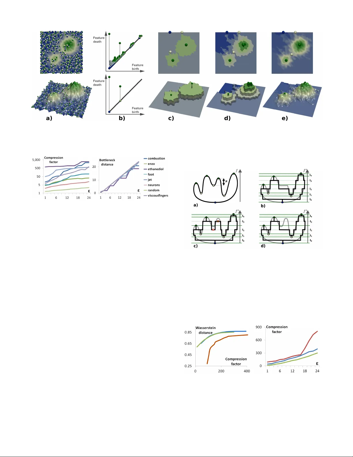
T opologically Contr olled Lossy Compression Maxime Soler * T otal S.A., F rance. Sorbonne Universit ´ e, CNRS, Laboratoire d’Inf ormatique de P aris 6, F-75005 Paris, F rance . M ´ elanie Plainchault † T otal S.A., F rance. Bruno Conche ‡ T otal S.A., F rance. Julien Tierny § Sorbonne Universit ´ e, CNRS, Laboratoire d’Inf ormatique de P aris 6, F-75005 Paris, F rance . A B S T R AC T This paper presents a new algorithm for the lossy compression of scalar data defined on 2D or 3D regular grids, with topological con- trol. Certain techniques allo w users to control the pointwise error induced by the compression. Howe v er , in many scenarios it is desirable to control in a similar way the preservation of higher-level notions, such as topological features , in order to provide guarantees on the outcome of post-hoc data analyses. This paper presents the first compression technique for scalar data which supports a strictly controlled loss of topological features. It pro vides users with specific guarantees both on the preserv ation of the important features and on the size of the smaller features destroyed during compression. In particular , we present a simple compression strategy based on a topo- logically adaptiv e quantization of the range. Our algorithm provides strong guarantees on the bottleneck distance between persistence diagrams of the input and decompressed data, specifically those associated with extrema. A simple extension of our strategy addi- tionally enables a control on the pointwise error . W e also show ho w to combine our approach with state-of-the-art compressors, to fur- ther improve the geometrical reconstruction. Extensive e xperiments, for comparable compression rates, demonstrate the superiority of our algorithm in terms of the preserv ation of topological features. W e show the utility of our approach by illustrating the compatibility between the output of post-hoc topological data analysis pipelines, ex ecuted on the input and decompressed data, for simulated or ac- quired data sets. W e also provide a lightweight VTK-based C++ implementation of our approach for reproduction purposes. 1 I N T R O D U C T I O N Data compression is an important tool for the analysis and visu- alization of large data sets. In particular , in the context of high performance computing, current trends and predictions [39] indicate increases of the number of cores in super-computers which e v olve faster than their memory , IO and network bandwidth. This observa- tion implies that such machines tend to compute results faster than they are able to store or transfer them. Thus, data movement is no w recognized as an important bottleneck which challenges large-scale scientific simulations. This challenges ev en further post-hoc data exploration and interacti ve analysis, as the output data of simulations often needs to be transferred to a commodity workstation to conduct such interactiv e inspections. Not only such a transfer is costly in terms of time, but data can often be too large to fit in the memory of a workstation. In this conte xt, data reduction and compression techniques are needed to reduce the amount of data to transfer . While many lossless compression techniques are now well estab- lished [25, 33, 47, 48], scientific data sets often need to be compressed * E-mail: soler .maxime@total.com † E-mail: melanie.plainchault@total.com ‡ E-mail: bruno.conche@total.com § E-mail: julien.tierny@lip6.fr at more aggressive rates, which requires lossy techniques [28, 31] (i.e. compression which alters the data). In the context of post-hoc analysis and visualization of data which has been compressed with a lossy technique, it is important for users to understand to what extent their data has been altered, to mak e sure that such an alteration has no impact on the analysis. This motiv ates the design of lossy compression techniques with error guarantees. Sev eral lossy techniques with guarantees hav e been documented, with a particular focus on pointwise error [12, 27, 33]. Howev er , pointwise error is a lo w level measure and it can be difficult for users to apprehend its propagation through their analysis pipeline, and consequently its impact on the outcome of their analysis. Therefore, it may be desirable to design lossy techniques with guarantees on the preservation of higher-le v el notions, such as the features of interest in the data. Howe ver , the definition of features primarily depends on the target application, but also on the type of analysis pipeline under consideration. This motiv ates, for each possible feature defini- tion, the design of a corresponding lossy compression strategy with guarantees on the preservation of the said features. In this work, we introduce a lossy compression technique that guarantees the preser - vation of features of interest, defined with topological notions, hence providing users with strong guarantees when post-analyzing their data with topological methods. T opological data analysis techniques [13, 23, 35] have demon- strated their ability over the last two decades to capture in a generic, robust and ef ficient manner features of interest in scalar data, for many applications: turbulent combustion [5], computational fluid dynamics [16], chemistry [18], astrophysics [40], etc. One reason for the success of topological methods in applications is the possi- bility for domain experts to easily translate high le vel notions into topological terms. For instance, the cosmic web in astrophysics can be extracted by querying the most persistent one-dimensional separatrices of the Morse-Smale complex connected to maxima of matter density [40]. Many similar feature definitions in topological terms can be found in the above application examples. For instance, we detail in Sect. 5.3 two analysis pipelines based on topological methods for the segmentation of acquired and simulated data. In the first case, features of interest (bones in a medical CT scan) can be extracted as the regions of space corresponding to the arcs of the split tree [8] which are attached to local maxima of CT intensity . In this scenario, it is important that lossy compression alters the data in a way that guarantees to preserve the split tree, to guarantee a faithful segmentation despite compression and thus, to enable further measurement, analysis and diagnosis ev en after compression. Thus, it is necessary, for all applications inv olving topological methods in their post-hoc analysis, to design lossy compression techniques with topological guarantees. This paper presents, to the best of our kno wledge, the first lossy compression technique for scalar data with such topological guar- antees. In particular, we introduce a simple algorithm based on a topologically adaptiv e quantization of the data range. W e carefully study the stability of the persistence diagram [11, 14] of the decom- pressed data compared to the original one. Gi ven a target feature size to preserve, which is expressed as a persistence threshold ε , our algorithm e xactly preserves the critical point pairs with persis- tence greater than ε and destroys all pairs with smaller persistence. W e provide guarantees on the bottleneck and W asserstein distances between the persistence diagrams, expressed as a function of the input parameter ε . Simple extensions to our strategy additionally enable to include a control on the pointwise error and to combine our algorithm with state-of-the-art compressors to impro ve the geometry of the reconstruction, while still providing strong topological guar- antees. Extensi ve e xperiments, for comparable compression rates, demonstrate the superiority of our technique for the preservation of topological features. W e show the utility of our approach by illustrating the compatibility between the output of topological anal- ysis pipelines, ex ecuted on the original and decompressed data, for simulated or acquired data (Sect. 5.3). W e also provide a VTK-based C++ implementation of our approach for reproduction purposes. 1.1 Related w ork Related existing techniques can be classified into two main cate- gories, addressing lossless and lossy compression respectiv ely . Regarding lossless compression, several general purpose algo- rithms hav e been documented, using entropy encoders [6, 17, 24, 25], dictionaries [47, 48] and predictors [7, 10]. For instance, the compres- sors associated with the popular file format Zip rely on a combination of the LZ77 algorithm [47] and Huffman coding [25]. Such com- pressors replace recurrent bit patterns in the data by references to a single copy of the pattern. Thus, these approaches reach particularly high compression rates when a high redundancy is present in the data. Se veral statistical [26, 33] or non-statistical [36] approaches hav e been proposed for volume data b ut often achie ve insuf ficient compression rates in applications (belo w two [31]), hence motiv ating lossy compression techniques. Regarding lossy compression, many strategies hav e been docu- mented. Some of them are now well established and implemented in international standards, such as GIF or JPEG. Such approaches rely for instance on vector quantization [37] or discrete cosine [29] and related block transforms [31]. Howe ver , relatively little work, mostly related to scientific computing applications, has yet focused on the definition of lossy compression techniques with an empha- sis on error control, mostly e xpressed as a bound on the pointwise error . For instance, though initially introduced for lossless com- pression, the FPZIP compressor [33] supports truncation of floating point values, thus providing an explicit relati ve error control. The Isabela compressor [28] supports predicti ve temporal compression by B-spline fitting and analysis of quantized error. The fixed rate compressor ZFP [31], based on local block transforms, supports maximum error control by not ignoring transform coef ficients whose effect on the output is more than a user defined error threshold [32]. More recently , Di and Cappello [12] introduced a compressor based on curve fitting specifically designed for pointwise error control. This control is enforced by explicitly storing values for which the curve fitting exceeds the input error tolerance. Iverson et al. [27] also introduced a compressor , named SQ , specifically designed for absolute error control. It supports a variety of strategies based on range quantization and/or region gro wing with an error-based stop- ping condition. For instance, giv en an input error tolerance ε , the quantization approach segments the range in contiguous intervals of width ε . Then, the scalar value of each grid vertex is encoded by the identifier of the interval it projects to in the range. At decom- pression, all vertices sharing a unique interv al identifier are given a common scalar value (the middle of the corresponding interv al), ef- fectiv ely guaranteeing a maximum error of ε (for vertices located in the vicinity of an interv al bound). Such a range quantization strategy is particularly appealing for the preservation of topological features, as one of the ke y stability results on persistence diagrams [14] states that the bottleneck distance between the diagrams of two scalar func- tions is bounded by their maximum pointwise error [11]. Intuitively , this means that all critical point pairs with persistence higher than ε in the input will still be present after a compression based on range quantization. Howe ver , a major drawback of such a strategy is the constant quantization step size, which implies that large parts of the range, possibly de void of important topological features, will still be decomposed into contiguous interv als of width ε , hence drastically limiting the compression rate in practice. In contrast, our approach is based on a topologically adapti ve range quantization which pre- cisely addresses this drawback, enabling superior compression rates. We additionally show how to extend our approach with absolute pointwise error control. As detailed in Sec. 3.3, this strategy pre- serves persistence pairs with persistence larger than ε , exactly . In contrast, since it snaps v alues to the middle of intervals, simple range quantization [27] may alter the persistence of critical point pairs in the decompressed data, by increasing the persistence of smaller pairs (noise) and/or decreasing that of lar ger pairs (features). Such an alteration is particularly concerning for post-hoc analyses, as it degrades the separation of noise from features and prev ents a reliable post-hoc multi-scale analysis, as the preserv ation of the persistence of critical point pairs is no longer guaranteed. Finally , note that a few approaches also considered topological aspects [2, 3, 41] but for the compression of meshes, not of scalar data. 1.2 Contributions This paper makes the follo wing new contributions: 1. A pproach: W e present the first algorithm for data compres- sion specifically designed to enforce topological control. W e present a simple strategy and carefully describe the stability of the persistence diagram of the output data. In particular , we show that, gi ven a target feature size (i.e. persistence) to preserve, our approach minimizes both the bottleneck and W asserstein distances between the persistence diagrams of the input and decompressed data. 2. Extensions: W e sho w ho w this strategy can be easily extended to additionally include control on the maximum pointwise error . Further, we sho w how to combine our compressor with state-of-the-art compressors, to improv e the av erage error . 3. A pplication: W e present applications of our approach to post- hoc analyses of simulated and acquired data, where users can faithfully conduct adv anced topological data analysis on com- pressed data, with guarantees on the maximal size of missing features and the exact preservation of the most important ones. 4. Implementation: W e provide a lightweight VTK-based C++ implementation of our approach for reproduction purposes. 2 P R E L I M I N A R I E S This section briefly describes our formal setting and presents an ov erview of our approach. An introduction to topological data analysis can be found in [13]. 2.1 Backgr ound Input data: W ithout loss of generality , we assume that the input data is a piecewise linear (PL) scalar field f : M → R defined on a PL d -manifold M with d equals 2 or 3. It has value at the vertices of M and is linearly interpolated on the simplices of higher dimen- sion. Adjacency relations on M can be described in a dimension independent way . The star St ( v ) of a vertex v is the set of simplices of M which contain v as a face. The link Lk ( v ) is the set of faces of the simplices of St ( v ) which do not intersect v . The topology of M can be described with its Betti numbers β i (the ranks of its homology groups [13]), which correspond in 3D to the numbers of connected components ( β 0 ), non collapsible cycles ( β 1 ) and voids ( β 2 ). Critical points: For visualization and data analysis purposes, se v- eral low-lev el geometric features can be defined giv en the input Figure 1: Cr itical points (spheres, blue: minima, white: saddles, g reen: maxima) and persistence diagrams of a clean (top) and noisy (bottom) 2D scalar field (from blue to green). F rom left to right: original 2D data, 3D terrain representation, persistence diag ram. The diagrams clearly exhibit in both cases two large pairs, corresponding to the two main hills. In the noisy diagram (bottom), small bars near the diagonal correspond to noisy features in the data. In this scenario, the bottleneck distance between the diagrams is the persistence of the largest unmatched feature (red pair in the zoomed inset, center right) while the Wasserstein distance is the sum of the persistence of all unmatched pairs. data. Giv en an isovalue i ∈ R , the sub-level set of i , noted f − 1 − ∞ ( i ) , is defined as the pre-image of the open interv al ( − ∞ , i ) onto M through f : f − 1 − ∞ ( i ) = { p ∈ M | f ( p ) < i } . Symmetrically , the sur- level set f − 1 + ∞ ( i ) is defined by f − 1 + ∞ ( i ) = { p ∈ M | f ( p ) > i } . These two objects serve as fundamental se gmentation tools in many analy- sis tasks [5]. The points of M where the Betti numbers of f − 1 − ∞ ( i ) change are the critical points of f (Fig. 1) and their associated f val- ues are called critical values . Let Lk − ( v ) be the lower link of the v er- tex v : Lk − ( v ) = { σ ∈ Lk ( v ) | ∀ u ∈ σ : f ( u ) < f ( v ) } . The upper link Lk + ( v ) is given by Lk + ( v ) = { σ ∈ Lk ( v ) | ∀ u ∈ σ : f ( u ) > f ( v ) } . T o classify Lk ( v ) without ambiguity into either lower or upper links, the restriction of f to the vertices of M is assumed to be injec- tiv e. This is easily enforced in practice by a variant of simulation of simplicity [15]. This is achieved by considering an associated injectiv e integer offset O f ( v ) , which initially typically corresponds to the vertex position offset in memory . Then, when comparing two vertices, if these share the same value f , their order is disam- biguated by their offset O f . A verte x v is regular , if and only if both Lk − ( v ) and Lk + ( v ) are simply connected. Otherwise, v is a critical point of f . Let d be the dimension of M . Critical points can be classified with their index I , which equals 0 for minima ( Lk − ( v ) = / 0 ), 1 for 1-saddles ( β 0 ( Lk − ( v )) = 2 ), ( d − 1 ) for ( d − 1 ) - saddles ( β 0 ( Lk + ( v )) = 2 ) and d for maxima ( Lk + ( v ) = / 0 ). V ertices for which β 0 ( Lk − ( v )) or β 0 ( Lk + ( v )) are greater than 2 are called de generate saddles . Persistence diagrams: The distribution of critical points of f can be represented visually by a topological abstraction called the per - sistence diagr am [11, 14] (Fig. 1). By applying the Elder Rule [13], critical points can be arranged in a set of pairs, such that each crit- ical point appears in only one pair ( c i , c j ) with f ( c i ) < f ( c j ) and I ( c i ) = I ( c j ) − 1 . Intuiti vely , the Elder Rule [13] states that if two topological features of f − 1 − ∞ ( i ) (for instance two connected com- ponents) meet at a giv en saddle c j of f , the youngest of the two features (the one created last) dies at the adv antage of the oldest. For example, if two connected components of f − 1 − ∞ ( i ) merge at a saddle c j , the one created by the highest minimum c i (the youngest one) is considered to die at c j , and c i and c j will form a critical point pair . The persistence diagram D ( f ) embeds each pair ( c i , c j ) in the plane such that its horizontal coordinate equals f ( c i ) , and the vertical coordinate of c i and c j are f ( c i ) and f ( c j ) , corresponding respectiv ely to the birth and death of the pair. The height of the pair P ( c i , c j ) = | f ( c j ) − f ( c i ) | is called the persistence and denotes the life-span of the topological feature created in c i and destroyed in c j . Thus, features with a short life span (noise) will appear in D ( f ) as low persistence pairs near the diagonal (Fig. 1, bottom). In low dimension, the persistence of the pairs linking critical points of index ( 0 , 1 ) , (( d − 1 ) , d ) and ( 1 , 2 ) (in 3D) denotes the life-span of con- nected components, voids and non-collapsible c ycles of f − 1 − ∞ ( i ) . In the rest of the paper , when discussing persistence diagrams, we will only consider critical point pairs of index ( 0 , 1 ) and (( d − 1 ) , d ) . The impact of this simplification is discussed in Sec. 5.4. In practice, per - sistence diagrams serve as an important visual representation of the distribution of critical points in a scalar data-set. Small oscillations in the data due to noise will typically be represented by critical point pairs with low persistence, in the vicinity of the diagonal. In contrast, topological features that are the most prominent in the data will be associated with large vertical bars (Fig. 1). In many applications, persistence diagrams help users as a visual guide to interactively tune simplification thresholds in topology-based, multi-scale data segmentation tasks based on the Reeb graph [9, 19, 34, 42, 45] or the Morse-Smale complex [21, 22]. Distance: In order to evaluate the quality of compression algorithms, sev eral metrics have been defined to ev aluate the distance between the decompressed data, noted g : M → R , and the input data, f : M → R . The p -norm, noted || f − g || p , is a classical example: || f − g || p =  ∑ v ∈ M | f ( v ) − g ( v ) | p  1 p (1) T ypical v alues of p with practical interests include p = 2 and p → ∞ . In particular, the latter case, called the maximum norm , is used to estimate the maximum pointwise error: || f − g || ∞ = max v ∈ M | f ( v ) − g ( v ) | (2) In the compression literature, a popular metric is the the P eak Signal to Noise Ratio (PSNR), where | σ 0 | is the number of vertices in M : PSN R = 20 l og 10  p | σ 0 | 2 × max v ∈ M f ( v ) − min v ∈ M f ( v ) || f − g || 2  (3) In the context of topological data analysis, several metrics [11] hav e been introduced too, in order to compare persistence diagrams. In our context, such metrics will be instrumental to evaluate the preservation of topological features after decompression. The bot- tleneck distance [11], noted d B ∞  D ( f ) , D ( g )  , is a popular exam- ple. Persistence diagrams can be associated with a pointwise dis- tance, noted d ∞ inspired by the ∞ -norm. Giv en two critical points p = ( p x , p y ) ∈ D ( f ) and q = ( q x , q y ) ∈ D ( g ) , d ∞ is defined as: d ∞ ( p , q ) = max ( | p x − q x | , | p y − q y | ) (4) Assume that the number of critical points of all possible index I is the same in both D ( f ) and D ( g ) . Then the bottleneck distance d B ∞  D ( f ) , D ( g )  can be defined as follows: d B ∞  D ( f ) , D ( g )  = min φ ∈ Φ  max p ∈ D ( f )  d ∞  p , φ ( p )    (5) where Φ is the set of all possible bijections φ mapping the critical points of D ( f ) to critical points of the same index I in D ( g ) . If the Figure 2: Overview of our topologically controlled lossy compression scheme on a 2D elevation example. First the input data f : M → R is pre-simplified into a function f 0 ((a), from top to bottom) to remov e all topological features below a user persistence tolerance ε (as illustrated by the persistence diagram (b)). The compression is achieved b y a topologically adaptive quantization of the range , which is segmented along the critical values of f 0 (c). A quantized function f 00 is constructed ((c), bottom) to only use a finite set of possible data values for regular v er tices, hence guaranteeing data compression, while still enf orcing or iginal v alues at cr itical points. This approach can be extended with point wise error control ((d)), by refining each quantization inter v al of f 0 larger than a target width ((d), bottom). Moreov er , our approach can be combined with any third par ty compressor (e) to further improve the geometry of the compressed data. numbers of critical points of index I do not match in both diagrams, φ will be an injection from the smaller set of critical points to the larger one. Additionally , φ will collapse the remaining, unmatched, critical points in the lar ger set by mapping each critical point c i to the other extremity of its persistence pair c j , in order to still penalize the presence of unmatched, low persistence features. Intuitiv ely , in the context of scalar data compression, the bot- tleneck distance between two persistence diagrams can be usually interpreted as the maximal size of the topological features which hav e not been maintained through compression (Fig. 1). A simple variant of the bottleneck distance, that is slightly more informativ e in the context of data compression, is the W asserstein distance, noted d W ∞ (sometimes called the Earth Mover’ s Distance [30]), between the persistence diagrams D ( f ) and D ( g ) : d W ∞  D ( f ) , D ( g )  = min φ ∈ Φ  ∑ p ∈ D ( f )  d ∞  p , φ ( p )    (6) In contrast to the bottleneck distance, the W asserstein distance will take into account the persistence of all the pairs which have not been maintained through compression (not only the largest one). 2.2 Overview An overvie w of our compression approach is presented in Fig. 2. First, the persistence diagram of the input data f : M → R is com- puted so as to ev aluate noisy topological features to later discard. The diagram consists of all critical point pairs of index ( 0 , 1 ) and ( d − 1 , d ) . Next, giv en a target size for the preservation of topological features, e xpressed as a persistence threshold ε , a simplified function f 0 : M → R is reconstructed [46] from the persistence diagram of f , D ( f ) , from which all persistence pairs below ε hav e been removed (Fig. 2(a)). Next, the image of M , f 0 ( M ) , is segmented along each critical value of f 0 . A new function f 00 : M → R is then obtained from f 0 by assigning to each verte x the mid-value of the interv al it maps to. This constitutes a topologically adaptive quantization of the range (Fig. 2(c)). This quantization can optionally be further subdivided to enforce a maximal pointwise error (Fig. 2(d)). At this point, the data can be compressed by storing the list of critical values of f 00 and storing for each verte x the identifier of the interv al it maps to. Optionally , the input data f can be compressed independently by state-of-the-art compressors, such as ZFP [31] (Fig. 2(e)). At decompression, a first function g 0 : M → R is constructed by re-assigning to each verte x the mid-value of the interv al it maps to. Optionally , if the data has been compressed with a third-party compressor , such as ZFP [31], at decompression, each vertex v alue is cropped to the extent of the interval it should map to. Last, a function g : M → R is reconstructed from the prescribed critical points of f 0 [46], to remov e any topological feature resulting from compression artifacts. 3 D AT A C O M P R E S S I O N This section presents our topologically controlled compression scheme. In addition to topological control (Sec. 3.1), our approach can optionally support pointwise error control (Sec. 3.3) as well as combinations with existing compressors (Sec. 3.4). The format of the files generated by our compressor is described in Sec. 3.2. 3.1 T opological control The input of our algorithm is the input data, f : M → R , as well as the size of the topological features to preserve through compression. This size is expressed as a persistence threshold ε . First, the persistence diagram of the input data, noted D ( f ) is computed. Next, a simplified version of the input data, noted f 0 : M → R , is constructed such that f 0 admits a persistence diagram which corresponds to that of f , but from which the critical point pairs with persistence smaller than ε hav e been removed. This simplification is achieved by using the algorithm by T ierny and Pascucci [46], which iterativ ely reconstructs sub-level sets to satisfy topological constraints on the extrema to preserve. In particular, this algorithm is gi ven as constraints the e xtrema of f to preserve, which are in our current setting the critical points inv olved in pairs with persistence larger than ε . In such a scenario, this algorithm has been shown to reconstruct a function f 0 such that || f − f 0 || ∞ ≤ ε [46]. At this point, f 0 carries all the necessary topological information that should be preserved through compression. In order to compress the data, we adopt a strategy based on range quantization. By assigning only a small number n of possible data values on the vertices of M , only l og 2 ( n ) bits should be required in principle for the storage of each v alue (instead of 64 for traditional floating point data with double precision). Moreover , encoding the data with a limited number of possible values is known to constitute a highly fa vorable configuration for post-process lossless compression, which achiev es high compression rates for redundant data. The difficulty in our context is to define a quantization that re- spects the topology of f 0 , as described by its persistence diagram Figure 3: T opologically controlled compression with pointwise error control. When pre-simplifying the input data f : M → R (left) into f 0 (center), the v alue variation of each simplified extrem um e equals the persistence P of the pair it belongs to , which is bounded by con- struction by ε : | f ( e ) − f 0 ( e ) | = P ≤ ε [11, 46]. When adding pointwise error control, each interval is subdivided such that its width does not exceed ε (right). Thus, when constructing the quantized function f 00 which maps each v er te x to the middle of its interval, each simplified extrem um e of f may fur ther move by a snapping distance s to the middle of its interval, which is itself bounded b y half the width of the interval ( ε / 2 ). Thus, | f ( e ) − f 00 ( e ) | = P + s ≤ ε + ε / 2 . D ( f 0 ) . T o do so, we collect all critical values of f 0 and segment the image of M by f 0 , noted f 0 ( M ) , into a set of contiguous interv als I = { I 0 , I 1 , . . . I n } , all delimited by the critical values of f 0 (Fig. 2, second column, top). Next, we create a ne w function f 00 : M → R , where all critical points of f 0 are maintained at their corresponding critical value and where all re gular vertices are assigned to the mid- value of the interv al I i they map to. This constitutes a topologically adaptiv e quantization of the range: only n possible values will be assigned to regular vertices. Note that although we modify data val- ues in the process, the critical vertices of f 0 are still critical vertices (with identical indices) in f 00 , as the lower and upper links (Sec. 2.1) of each critical point are preserved by construction. 3.2 Data encoding The function f 00 is encoded in a two step process. First a topological index is created. This index stores the identifier of each critical verte x of f 00 as well as its critical value, and for each of these, the identifier i of the interval I i immediately abov e it if and only if some vertices of M indeed project to I i through f 00 . This strategy enables the sav e of identifiers for empty intervals. The second step of the encoding focuses on data v alues of regular vertices of f 00 . Each vertex of M is assigned the identifier i of the interval I i it projects to through f 00 . For n v vertices and n i non-empty intervals between n c critical points, we store per-v ertex interval identifiers ( n v words of log 2 ( n i ) bits), critical point positions in a verte x index ( n c words of log 2 ( n v ) bits), critical types ( n c words of 2 bits) and critical values ( n c floats). Since it uses a finite set of data values, the buf fer storing interval assignments for all vertices of M is highly redundant. Thus, we further compress the data (topological index and interval assignment) with a standard lossless compressor ( Bzip2 [38]). 3.3 P ointwise error control Our approach has been designed so far to preserv e topological fea- tures thanks to a topologically adaptiv e quantization of the range. Howe ver , this quantization may be composed of arbitrarily large intervals, which may result in lar ge pointwise error . Our strategy can be easily extended to optionally support a maxi- mal pointwise error with regard to the input data f : M → R , still controlled by the parameter ε . In particular, this can be achie ved by subdividing each interval (Sec. 3.1) according to a tar get maximal width w , prior to the actual quantization and data encoding (Sec. 3.2). Since the topologically simplified function f 0 is guaranteed to be at most ε -away from f ( || f − f 0 || ∞ ≤ ε , Sec. 3.1), further subdividing each interval with a maximum authorized width of w will result in a maximum error of ε + w / 2 when quantizing the data into f 00 . For instance, a local maximum of f of persistence lo wer than ε can be pulled down by at most ε when simplifying f into f 0 [46] (Fig. 3, center) and then further pulled down by up to w / 2 when being as- signed the mid-value of its new interval (of width w , Fig. 3, right). In practice, for simplicity , we set w = ε . Hence, a maximum pointwise error of 3 ε / 2 is guaranteed at compression ( || f − f 00 || ∞ ≤ 3 ε / 2). 3.4 Combination with state-of-the-ar t compressors The compression approach we presented so f ar relies on a topolog- ically adaptive quantization of the range (with optional pointwise error control). The compression is achiev ed by only allo wing a small number of possible scalar values in the compressed data, which may typically result in noticeable stair case artifacts. T o address this, our method can be optionally combined seamlessly with any state-of-the- art lossy compressor . For our experiments, we used ZFP [31]. Such a combination is straightforward at compression time. In particu- lar , in addition to the topological index and the compressed quanta identifiers (Sect. 3.2), the input data f : M → R is additionally and independently compressed by the third-party compressor ( ZFP ). 4 D AT A D E C O M P R E S S I O N This section describes the decompression procedure of our approach, which is symmetric to the compression pipeline described in the previous section (Sec. 3). This section also further details the guar- antees provided by our approach re garding the bottleneck ( d B ∞ ) and W asserstein ( d W ∞ ) distances between the persistence diagrams of the input data and the decompressed data, noted g : M → R (Sec. 4.4). 4.1 Data decoding First, the compressed data is decompressed with the lossless decom- pressor Bzip2 [38]. Next, a function g 0 : M → R is constructed based on the topological index and the interval assignment buf fer (Sec. 3.2). In particular, each critical verte x is assigned its critical value (as stored in the topological index) and regular vertices are assigned the mid-v alue of the interv al they project to, based on the interval assignment b uffer (Sec. 3.2). 4.2 Combination with state-of-the-ar t decompressors If a state-of-the-art compression method has been used in conjunc- tion with our approach (Sec. 3.4), we use its decompressor to gen- erate the function g 0 : M → R . Next, for each verte x v of M , if g 0 ( v ) is outside of the interval I i where v is supposed to project, we snap g 0 ( v ) to the closest extremity of I i . This guarantees that the decompressed data respects the topological constraints of D ( f 0 ) , as well as the optional target pointwise error (Sec. 3.3). 4.3 T opological reconstruction The decompressed function g 0 may contain at this point extraneous critical point pairs, which were not present in D ( f 0 ) (Sec. 3.1). For instance, if a state-of-the-art compressor has been used in conjunc- tion with our approach, arbitrary oscillations within a given interv al I i can still occur and result in the apparition of critical point pairs in D ( g 0 ) (with a persistence smaller than the target interval width w , Sec. 3.3) which were not present in D ( f 0 ) . The presence of such persistence pairs impacts the distance metrics introduced in Sec. 2.1, and therefore impacts the quality of our topology controlled com- pression. Thus, such pairs need to be simplified in a post-process. Note that, ev en if no third-party compressor has been used, since our approach is based on a topologically adaptive quantization of the range, large flat plateaus will appear in g 0 . Depending on the vertex offset O g 0 : M → R (used to disambiguate flat plateaus, Sec. 2.1), arbitrarily small persistence pairs can also occur . Therefore, for such flat plateaus, O g 0 must be simplified to guarantee its monotonicity ev erywhere except at the desired critical v ertices (i.e. those stored in the topological index, Sec. 3.2). Thus, whether a state-of-the-art compressor has been used or not, the last step of our approach consists in reconstructing the function g : M → R from g 0 by enforcing the critical point constraints of f 0 (stored in the topological index) with the algorithm by T ierny and Pascucci [46]. Note that this algorithm will automatically resolve flat plateaus, by enforcing the monotonicity of O g ev erywhere except at the prescribed critical points [46]. Therefore, the ov erall output of our decompression procedure is the scalar field g : M → R as well as its corresponding verte x integer of fset O g : M → N . 4.4 T opological guarantees The last step of our decompression scheme, topological reconstruc- tion (Sec. 4.3), guarantees that D ( g ) admits no other critical points than those of D ( f 0 ) (specified in the topological index). More- ov er , the corresponding critical values hav e been strictly enforced (Sec. 4.1). This guarantees that d B ∞  D ( g ) , D ( f 0 )  = 0, and thus: d B ∞  D ( g ) , D ( f )  ≤ d B ∞  D ( g ) , D ( f 0 )  + d B ∞  D ( f 0 ) , D ( f )  ≤ d B ∞  D ( f 0 ) , D ( f )  (7) Since we know that f 0 is ε -away from the original data f (Sec. 3.1) and due to persistence diagrams stability [11], we then hav e: d B ∞  D ( g ) , D ( f )  ≤ || f − f 0 || ∞ ≤ ε (8) Thus, the bottleneck distance between the persistence diagrams of the input and decompressed data is indeed bounded by ε , which happens to precisely describe the size of the topological features that the user wants to preserve through compression. Since D ( f 0 ) ⊂ D ( f ) and d B ∞  D ( g ) , D ( f 0 )  = 0 , we have D ( g ) ⊂ D ( f ) . This further implies that: d B ∞  D ( g ) , D ( f )  = max ( p , q ) ∈  D ( g ) 4 D ( f )  P ( p , q ) (9) where P ( p , q ) denotes the persistence of a critical point pair ( p , q ) and where D ( g ) 4 D ( f ) denotes the symmetric difference between D ( g ) and D ( f ) (i.e. the set of pairs present in D ( f ) but not in D ( g ) ). In other words, the bottleneck distance between the persistence diagrams of the input and decompressed data exactly equals the persistence of the most persistent pair present in D ( f ) but not in D ( g ) (in red in Fig. 1). This guarantees the exact preservation of the topological features selected with an ε persistence threshold. As for the W asserstein distance, with the same rationale, we get: d W ∞  D ( g ) , D ( f )  = ∑ ( p , q ) ∈  D ( g ) 4 D ( f )  P ( p , q ) (10) In other words, the W asserstein distance between the persistence diagrams of the input and decompressed data will be exactly equal to sum of the persistence of all pairs present in D ( f ) but not in D ( g ) (small bars near the diagonal in Fig. 1, bottom), which corresponds to all the topological features that the user precisely wanted to discard. Finally , for completeness, we recall that, if pointwise error control was enabled, our approach guarantees || f − g || ∞ ≤ 3 ε / 2 (Sec. 3.3). 5 R E S U LTS This section presents experimental results obtained on a desktop computer with two Xeon CPUs (3.0 GHz, 4 cores each), with 64 GB of RAM. For the computation of the persistence diagram and the topological simplification of the data, we used the algorithms by T ierny and Pascucci [46] and Gueunet et al. [20], whose implemen- tations are av ailable in the T opology T oolKit (TTK) [43]. The other components of our approach (including bottleneck and W asserstein distance computations) hav e been implemented as TTK modules. Note that our approach has been described so far for triangulations. Howe ver , we restrict our experiments to regular grids in the follo w- ing as most state-of-the-art compressors (including ZFP [31]) hav e been specifically designed for regular grids. For this, we use the triangulation data-structure from TTK, which represents implicitly regular grids with no memory o verhead using a 6-tet subdi vision. Fig. 4 presents an ov erview of the compression capabilities of our approach on a noisy 2D example. A noisy data set is pro vided on the input. Given a user threshold on the size of the topological features to preserve, expressed as a persistence threshold ε , our approach generates decompressed data-sets that all share the same persistence diagram D ( g ) (Fig. 4(b), bottom), which is a subset of the diagram of the input data D ( f ) (Fig. 4(b), top) from which pairs with a persistence lower than ε hav e been removed, and those abov e ε hav e been exactly preserved. As shown in this example, augmenting our approach with pointwise error control or combining it with a state-of-the-art compressor allo ws for improved geometrical reconstructions, but at the expense of much lo wer compression rates. Note that the Fig. 4(e) sho ws the result of the compression with ZFP [31], which has been augmented with our topological control. This shows that our approach can enhance any existing compression scheme, by providing strong topological guarantees on the output. 5.1 Compression performance W e first ev aluate the performance of our compression scheme with topological control only on a variety of 3D data sets all sampled on 512 3 regular grids. Fig. 5 (left) presents the ev olution of the compression rates for increasing target persistence thresholds ε ex- pressed as percentages of the data range. This plot confirms that when fine scale structures need to be preserv ed (small ε values, left), smaller compression rates are achie ved, while higher compression rates (right) are reached when this constraint is relax ed. Compres- sion rates vary among data sets as the persistence diagrams v ary in complexity . The Ethane Diol dataset (topmost curve) is a very smooth function coming from chemical simulations. High com- pression factors are achiev ed for it, almost irrespectiv e of ε . On the contrary , the random dataset (bottom curve) exhibits a complex persistence diagram, and hence lower compression rates. In between, all data sets e xhibit the same increase in compression rate for increasing ε values. Their respective position between the two extreme configurations of the spectrum (ele vation and random) depend on their input topological comple xity (number of pairs in the persistence diagram). Fig. 5 (right) plots the e volution of the bottleneck distance between the input and decompressed data, d B ∞  D ( f ) , D ( g )  , for increasing target persistence threshold ε , for all data sets. This plot shows that all curves are located belo w the identity diagonal. This constitutes a practical v alidation of our guaranteed bound on the bot- tleneck distance (Eq. 8). Note that, for a gi ven data set, the proximity of its curve to the diagonal is directly dependent on its topological complexity . This result confirms the strong guarantees regarding the preservation of topological features through compression. T able 1 provides detailed timings for our approach and shows that most of the compression time (at least 75%, S column) is spent simplifying the original data f into f 0 (Sect. 3). If desired, this step can be skipped to drastically improv e time performance, but at the expense of compression rates (T able 1, right). Indeed, as shown in Fig. 6, skipping this simplification step at compression time results in quantized function f 00 that still admits a rich topology , T able 1: Detailed computation times on 512 3 regular grids ( ε = 5% ), with and without compression-time simplification. P , S , Q and L stand for the persistence diagram, topological simplification, topological quantization and lossless compression efforts (%). Data-set With compression-time simplification No simplification Decompr . P (%) S (%) Q (%) L (%) T otal (s) Compr . Rate T otal (s) Compr . Rate Time (s) Combustion 8.4 89.3 0.7 1.6 593.9 121.3 64.1 111.1 213.3 Elevation 14.6 84.1 1.2 0.1 157.0 174,848.0 25.3 174,848.0 211.5 EthaneDiol 12.6 86.7 0.5 0.2 490.0 2,158.6 63.0 2,158.6 228.9 Enzo 9.5 86.7 1.0 2.7 695.6 24.5 91.8 19.8 204.0 Foot 12.6 81.9 1.6 3.8 380.6 12.1 68.4 7.75 205.7 Jet 22.2 75.7 0.6 1.5 451.3 315.6 111.1 287.6 220.3 Random 15.9 76.0 2.8 5.3 1357.1 1.5 307.7 1.5 101.2 Figure 4: Compression of the noisy 2D data set from Fig. 1 ((a), 80,642 b ytes, top: 2D data, bottom: 3D terr ain). In all cases (c-e), our compression algorithm was configured to maintain topological features more persistent than 20% of the function range, as illustrated with the persistence diagrams ((b), top: original noisy data D ( f ) , bottom: decompressed data D ( g ) ). Our topology controlled compression (c), augmented with pointwise error control (d), and combined with ZFP [31] ((e), one bit per scalar) yields compression rates of 163, 50 and 14 respectiv ely . Figure 5: Perf or mance analysis of our compression scheme (topolog- ical control only). Left: Compression rate for various 3D data sets, as a function of the target persistence threshold ε (percentage of the function range). Right: Bottleneck distance between the persistence diagrams of the input and decompressed data, d B ∞  D ( f ) , D ( g )  , for increasing target persistence thresholds ε . and which therefore constitutes a less fav orable ground for the post- process lossless compression (higher entropy). Note howe ver that our implementation has not been optimized for ex ecution time. W e leav e time performance improvement for future work. 5.2 Comparisons Next, we compare our approach with topological control only to the SQ compressor [27], which has been explicitly designed to control pointwise error . Thus, it is probably the compression scheme that is the most related to our approach. SQ proposes two main strate gies for data compression, one which is a straight range quantization (with a constant step size ε , SQ-R ) and the other which grows re- gions in the 3D domain, within a target function interval width ε ( SQ-D ). Both variants, which we implemented ourselves, provide an explicit control on the resulting pointwise error ( || f − g || ∞ ≤ ε ). As such, thanks to the stability result on persistence diagrams [11], SQ also bounds the bottleneck distance between the persistence di- agrams of the input and decompressed data. Each pair completely included within one quantization step is indeed flattened out. Only the pairs larger than the quantization step size ε do surviv e through compression. Howe ver , the latter are snapped to admitted quantiza- tion values. In practice, this can artificially and arbitrarily reduce the persistence of certain pairs, and increase the persistence of oth- ers. This is particularly problematic as it can reduce the persistence of important features and increase that of noise, which prevents a reliable multi-scale analysis after decompression. This difficulty is one of the main motiv ations which led us to design our approach. T o evaluate this, we compare SQ to our approach in the light of the W asserstein distance between the persistence diagrams of the input Figure 6: T opologically controlled compression with (b) and without (c) compression-time simplification. T opological simplification (c to d) remov es all critical point pairs not present in the topological index (red circles) and exactly maintains the others [46]. Thus, simplifying the data only at decompression (d) yields identical decompressed data (d vs b). The quantized function then admits a richer topology (c vs b), which deteriorates compression rates. Figure 7: Compar ison to the SQ compressor [27] (green: SQ-D , blue: SQ-R, red: our approach). Left: aver age nor maliz ed Wasserstein distance between the persistence diag rams of the input and decom- pressed data, for increasing compression rates. Right: av erage compression factors f or increasing target persistence thresholds ε . Figure 8: Augmenting a third party compressor , here ZFP [31] (1 bit per vertex v alue), with topological control. Left: Compression factors for increasing persistence targets ε . Right: PSNR for increasing persistence targets ε . In these plots (left and right), a persistence target of 100% indicates that no topological control was enforced. and decompressed data, d W ∞  D ( f ) , D ( g )  . As described in Sec. 2.1, this distance is more informati ve in the context of compression, since not only does it track all pairs which hav e been lost, but also the changes of the pairs which hav e been preserved. Fig. 7 (left) presents the ev olution of the W asssertein distance, averaged o ver all our data sets, for increasing compression rates. This plot shows that our approach (red curve) achie ves a significantly better preserv ation of the topological features than SQ , for all compression rates, especially for the lowest ones. As discussed in the previous paragraph, giv en a quantization step ε , SQ will preserve all pairs more persistent than ε but it will also de grade them, as shown in the abo ve experiment. Another drawback of SQ regarding the preserv ation of topological features is the compression rate. Since it uses a constant quantization step size, it may require many quantization interv als to preserve pairs abov e a target persistence ε , although large portions of the range may be de void of important topological features. T o illustrate this, we compare the compression rates achieved by SQ and our approach, for increasing values of the parameter ε . As in Fig. 5, increasing slopes can be observed. Ho wever , our approach always achieves higher compression rates, especially for larger persistence tar gets. Next, we study the capabilities offered by our approach to aug- ment a third party compressor with topological control (Secs. 3.4 and 4.2). In particular , we augmented the ZFP compressor [31], by using the original implementation provided by the author (with 1 bit per verte x v alue). Fig. 8 (left) indicates the e volution of the compression rates as the target persistence threshold ε increases. In particular , in these experiments, a persistence tar get of 100% indicates that no topological control was enforced. Thus, these curves indicate, apart from this point, the overhead of topological guarantees over the ZFP compressor in terms of data storage. These curves, as it could be expected with Fig. 5, show that compression rates will rapidly drop down for topologically rich data sets (such as the random one). On the contrary , for smoother data sets, such as Ethane Diol or Jet, high compression rates can be maintained. This shows that aug- menting a third party compressor with topological control results in compression rates that adapt to the topological complexity of the input. Fig. 8 (right) shows the evolution of the PSNR (Sec. 2.1) for decreasing persistence targets ε . Surprisingly , in this context, the enforcement of topological control impro ves the quality of the data decompressed with ZFP , with higher PSNR values for little persistence targets. This is due to the rather aggressive compression rate which we used for ZFP (1 bit per vertex v alue) which tends to add noise to the data. Thanks to our topological control (Sec. 4.3), such compression artifacts can be cleaned up by our approach. T able 2 ev aluates the advantage of our topology aware compres- sion ov er a standard lossy compression, followed at decompression by a topological cleanup (which simplifies all pairs less persistent than ε [46]). In particular, this table shows that augmenting a third party compressor (such as ZFP) with our topological control (second line) results in more faithful decompressed data (lo wer W asserstein distances to the original data) than simply executing the compressor and topologically cleaning the data in a post-process after decompres- Figure 9: T opology dr iv en data segmentation with multi-scale split trees, on the or iginal data (left) and the data compressed with our approach (right). Top to bottom: persistence diagrams, sliced views of the data, output segmentations. The analysis yields compatible outcomes with and without compression, as sho wn with the bottom row , which exhibits identical segmentations (compression rate: 360). sion (first line). This further motiv ates our approach for augmenting existing compressors with topological control. Finally , T able 3 provides a comparison of the running times (for comparable compression rates) between our approach and SQ and ZFP . ZFP has been designed to achiev e high throughput and thus deli vers the best time performances. The running times of our approach are on par with other approaches enforcing strong guarantees on the decompressed data (SQ-R and SQ-D). 5.3 Application to post-hoc topological data analysis A key motiv ation to our compression scheme is to allow users to faithfully conduct advanced topological data analysis in a post- process, on the decompressed data, with guarantees on the com- patibility between the outcome of their analysis and that of the same analysis on the original data. W e illustrate this aspect in this sub- section, where all examples ha ve been compressed by our algorithm, without pointwise error control nor combination with ZFP . W e first illustrate this in the conte xt of medical data segmentation with Fig. 9, which sho ws a foot scan. The persistence diagram of the original data counts more than 345 thousands pairs (top left). The split tree [5, 8] is a topological abstraction which trac ks the connected components of sur-le vel sets of the data. It has been shown to excel at segmenting medical data [9]. In this context, users typically compute multi-scale simplifications of the split tree to extract the most important features. Here, the user simplified the split tree until it counted only 5 leav es, corresponding to 5 features of interest (i.e. the 5 toes). Next, the se gmentation induced by the simplified split tree has been extracted by considering regions corresponding to T able 2: W asserstein distance between the persistence diagrams of the or iginal and decompressed data ( ε = 1% ). First line: ZFP 1bit/scalar , followed b y a topology cleanup procedure. Second line: ZFP 1bit/scalar , augmented with our approach. Data-set d W ∞ Combustion Elev ation EthaneDiol Enzo Foot Jet ZFP + Cleanup 18.08 0.00 1.53 189.66 520,371 351.97 T opology-aware ZFP 13.73 0.00 0.40 131.11 506,714 153.45 Figure 10: T opology driven data segmentation (r ight) on a viscous fingering simulation (left) on the original data (top) and the data com- pressed with our approach. Compatible fingers are extracted after compression (compression rate: 56). each arc connected to a leaf. This results immediately in the sharp segmentation of toe bones. (Fig. 9, bottom left). W e applied the exact same analysis pipeline on the data compressed with our approach. In particular , since it can be known a priori that this data has only 5 features of interest (5 toes), we compressed the data with a target persistence ε such that only 5 pairs remained in the persistence diagram (top right). Although such an aggressiv e compression greatly modifies data values, the outcome of the segmentation is identical (T able 4), for an approximate compression rate of 360. Next, we e valuate our approach on a more challenging pipeline (Fig. 10), where features of interest are not e xplicitly related to the persistence diagram of the input data. W e consider a snapshot of a simulation run of viscous fingering and apply the topological data analysis pipeline described by Fa velier et al. [16] for the extraction and tracking of viscous fingers. This pipeline first isolates the largest connected component of sur-lev el set of salt concentration. Next it considers its height function, on which persistent homology is applied to retrieve the deepest points of the geometry (corresponding to finger tips). Finally , a distance field is grown from the finger tips and the Morse complex of this distance field is computed to isolate fingers. In contrast to the previous example, the original data un- dergoes man y transformations and changes of representation before the extraction of topological features. Despite this, when applied to the data compressed with our scheme, the analysis pipeline still outputs consistent results with the original data (Fig. 10, compres- sion rate: 56). Only slight variations can be perceiv ed in the local geometry of fingers, but their number is unchanged and their overall geometry compatible. T able 4 provides a quantitati ve estimation of T able 3: Time performance comparison between ZFP , SQ and our approach on 512 3 regular grids. Data-set Time (s). ZFP SQ-R SQ-D Ours Combustion 4.6 37.6 242.9 64.1 Elev ation 7.2 31.4 204.2 25.3 EthaneDiol 4.7 34.4 197.1 63.0 Enzo 4.7 33.0 229.5 91.8 Foot 2.9 18.2 198.0 68.4 Jet 4.7 31.4 203.4 111.1 Random 4.1 31.6 182.7 307.7 the similarity between segmentations, before and after compression with sev eral algorithms. This table shows that our approach enables the computation of more faithful topological segmentations (higher rand index) compared to SQ and ZFP , which further underlines the superiority of our strategy at preserving topological features. 5.4 Limitations Like all lossy techniques, our approach is subject to an input param- eter that controls the loss, namely the persistence threshold ε abov e which features should be strictly preserv ed. While we believe this pa- rameter to be intuitiv e, prior domain kno wledge about the size of the features to preserve may be required. Howe ver , conservati ve values (typically 5% ) can be used by default, as they already achie ve high compression rates while preserving most of the features. In some applications, ad-hoc metrics [9] may be preferred o ver persistence. Our approach can be used in this setting too as the simplification algorithm that we use [46] supports an arbitrary selection of the critical points to preserve. Howe ver , it becomes more difficult then to express clear guarantees on the compression quality in terms of the bottleneck and W asserstein distances between the persistence diagrams of the input and decompressed data. When pointwise error control is enabled, the ∞ -norm between the input and decompressed data is guaranteed by our approach to be bounded by 3 ε / 2 . This is due to the topological simplification algorithm that we employ [46], which is a flooding-only algorithm. Alternativ es combining flood- ing and carving [4, 44] could be considered to reach a guaranteed ∞ -norm of ε . Finally , our approach only considers persistence pairs corresponding to critical points of index ( 0 , 1 ) and (d-1, d). Ho wev er ( 1 , 2 ) pairs may hav e a practical interest in certain 3D applications and it might be interesting to enforce their preservation throughout compression. This would require an efficient data reconstruction algorithm for ( 1 , 2 ) pairs, which seems challenging [1]. 6 C O N C L U S I O N In this paper , we presented the first compression scheme, to the best of our knowledge, which provides strong topological guarantees on the decompressed data. In particular , giv en a target topological feature size to preserve, e xpressed as a persistence threshold ε , our approach discards all persistence pairs belo w ε in order to achie ve high compression rates, while e xactly preserving persistence pairs abov e ε . Guarantees are given on the bottleneck and W asserstein distances between the persistence diagrams of the input and decom- pressed data. Such guarantees are key to ensure the reliability of an y post-hoc, possibly multi-scale, topological data analysis performed on decompressed data. Our approach is simple to implement; we provide a lightweight VTK-based C++ reference implementation. Experiments demonstrated the superiority of our approach in terms of topological feature preserv ation in comparison to existing compressors, for comparable compression rates. Our approach can be extended to include pointwise error control. Further , we showed, with the example of the ZFP compressor [31], how to make any third-party compressor become topology-awar e by combining it with our approach and making it benefit from our strong topological guarantees, without af fecting too much isosurface geometry. W e also showed that, when aggressi ve compression rates were selected, our topological approach could improve existing compressors in terms of PSNR by cleaning up topological compression artifacts. T able 4: Rand index between the outputs of a data segmentation pipeline based on topological methods (Sect. 5.3), before and after compression, for sev eral methods at compatible compression r ates. Experiment Rand index Ours SQ-R SQ-D ZFP Foot scan 1.000 0.913 0.895 0.943 V iscous fingers 0.985 0.977 0.977 0.973 W e finally showed the utility of our approach by illustrating, quali- tativ ely and quantitatively , the compatibility between the output of post-hoc topological data analysis pipelines, ex ecuted on the input and decompressed data, for simulated or acquired data sets. Our contribution enables users to faithfully conduct advanced topological data analysis on decompressed data, with guarantees on the size of missed features and the exact preserv ation of most prominent ones. In the future, we plan to improv e practical aspects of our algo- rithm for in-situ deployment and to handle time-varying datasets. Runtime limitations will be in vestigated, with the objecti ve to mit- igate the effects of using (or not) a sequential topological simpli- fication step, and to determine how many cores are necessary to outperform raw storage. A streaming version of the algorihm, which would not require the whole dataset to be loaded at once would be of great interest in this framework. Finally , as our approach focuses on regular grids, since, in the case of unstructured grids, the actual mesh is often the information that requires the most storage space, we will in vestigate mesh compression techniques with guarantees on topological feature preservation for scalar fields defined on them. A C K N OW L E D G M E N T S This work is partially supported by the Bpifrance grant “ A VIDO” (Programme d’In vestissements d’A venir, reference P112017-2661376/DOS0021427) and by the French National Association for Research and T echnology (ANR T), in the framework of the LIP6 - T otal SA CIFRE partnership reference 2016/0010. The authors would like to thank the anonymous re viewers for their thoughtful remarks and suggestions. R E F E R E N C E S [1] D. Attali, U. Bauer , O. Devillers, M. Glisse, A. Lieutier . Homological reconstruction and simplification in R3. SoCG , 117–126, 2013. [2] C. Bajaj D. Schikore. T opology preserving data simplification with error bounds. Computers and Graphics , 22(1):3–12, 1998. [3] C. L. Bajaj, V . Pascucci, G. Zhuang. Single resolution compression of arbitrary triangular meshes with properties. IEEE DC , 247–256, 1999. [4] U. Bauer , C. Lange, M. W ardetzky . Optimal topological simplification of discrete functions on surfaces. DCG , 47(2):347–377, 2012. [5] P . Bremer, G. W eber, J. Tiern y , V . Pascucci, M. Day , J. Bell. Interactiv e exploration and analysis of large scale simulations using topology- based data segmentation. IEEE TVCG , 17(9):1307–1324, 2011. [6] M. Burrows D. Wheeler . A block sorting lossless data compression algorithm. T echnical report, Digital Equipment Corporation, 1994. [7] M. Burtscher P . Ratanaworabhan. High throughput compression of double-precision floating-point data. 293–302, 2007. [8] H. Carr , J. Snoeyink, U. Axen. Computing contour trees in all dimen- sions. Symp. on Dis. Alg. , 918–926, 2000. [9] H. Carr , J. Snoe yink, M. van de Panne. Simplifying flexible isosurfaces using local geometric measures. IEEE VIS , 497–504, 2004. [10] J. Cleary I. W itten. Data compression using adapti ve coding and partial string matching. IEEE T rans. Comm. , 32(4):396–402, 1984. [11] D. Cohen-Steiner , H. Edelsbrunner, J. Harer . Stability of persistence diagrams. Symp. on Comp. Geom. , 263–271, 2005. [12] S. Di F . Cappello. Fast error-bounded lossy HPC data compression with SZ. IEEE Symp. on PDP , 730–739, 2016. [13] H. Edelsbrunner J. Harer . Computational T opology: An Introduction . American Mathematical Society , 2009. [14] H. Edelsbrunner , D. Letscher, A. Zomorodian. T opological persistence and simplification. Disc. Compu. Geom. , 28(4):511–533, 2002. [15] H. Edelsbrunner E. P . Mucke. Simulation of simplicity: a technique to cope with de generate cases in geometric algorithms. T oG , 9(1):66–104, 1990. [16] G. Fa velier, C. Gueunet, J. T ierny . V isualizing ensembles of viscous fingers. IEEE SciV is Contest , 2016. [17] S. W . Golomb . Run-length encodings. IEEE Tr ans. on IT , 12(3):399– 401, 1966. [18] D. Guenther, R. Alvarez-Boto, J. Contreras-Garcia, J.-P . Piquemal, J. T ierny . Characterizing molecular interactions in chemical systems. IEEE TVCG , 20(12):2476–2485, 2014. [19] C. Gueunet, P . Fortin, J. Jomier, J. Tierny . Contour forests: Fast multi-threaded augmented contour trees. IEEE LD A V , 85–92, 2016. [20] C. Gueunet, P . Fortin, J. Jomier, J. T ierny . T ask-based augmented merge trees with Fibonacci heaps. IEEE LDA V , 2017. [21] A. Gyulassy , P . T . Bremer , B. Hamann, V . Pascucci. A practical approach to morse-smale complex computation: Scalability and gener- ality . IEEE TVCG , 14(6):1619–1626, 2008. [22] A. Gyulassy , D. Guenther , J. A. Levine, J. T ierny , V . Pascucci. Con- forming morse-smale complexes. IEEE TVCG , 20(12):2595–2603, 2014. [23] C. Heine, H. Leitte, M. Hlawitschka, F . Iuricich, L. De Floriani, G. Scheuermann, H. Hagen, C. Garth. A survey of topology-based methods in visualization. Comp. Grap. F or . , 35(3):643–667, 2016. [24] P . G. Howard J. S. V itter. Analysis of arithmetic coding for data compression. IEEE DCC , 3–12, 1991. [25] D. Huffman. A method for the construction of minimum-redundancy codes. 40(9):1098–1101, 1952. [26] M. Isenbur g, P . Lindstrom, J. Snoeyink. Lossless Compression of Pre- dicted Floating-Point Geometry . Computer-Aided Design , 37(8):869– 877, 2005. [27] J. Iverson, C. Kamath, G. Karypis. Fast and effecti ve lossy compression algorithms for scientific datasets. Eur o-P ar , 843–856, 2012. [28] S. Lakshminarasimhan, N. Shah, S. Ethier, S. Klasky , R. Latham, R. B. Ross, N. F . Samatov a. Compressing the incompressible with ISABELA: in-situ reduction of spatio-temporal data. Eur o-P ar , 366–379, 2011. [29] N. K. Laurance D. M. Monro. Embedded DCT Coding with Signifi- cance Masking. IEEE ICASPP , 2717–2720, 1997. [30] E. Levina P . Bickel. The earthmov er’ s distance is the mallo ws distance: some insights from statistics. IEEE ICCV , vol. 2, 251–256, 2001. [31] P . Lindstrom. Fixed-rate compressed floating-point arrays. IEEE TVCG , 20(12):2674–2683, 2014. [32] P . Lindstrom, P . Chen, E. Lee. Reducing Disk Storage of Full-3D Seismic W aveform T omography (F3DT) through Lossy Online Com- pression. Computers & Geosciences , 93:45–54, 2016. [33] P . Lindstrom M. Isenb urg. Fast and ef ficient compression of floating- point data. IEEE TVCG , 12(5):1245–1250, 2006. [34] V . Pascucci, G. Scorzelli, P . T . Bremer , A. Mascarenhas. Robust on- line computation of Reeb graphs: simplicity and speed. T oG , 26(3):58, 2007. [35] V . Pascucci, X. T ricoche, H. Hagen, J. Tiern y . T opological Data Analy- sis and V isualization: Theory, Algorithms and Applications . Springer, 2010. [36] P . Ratanaw orabhan, J. Ke, M. Burtscher . Fast lossless compression of scientific floating-point data. IEEE Data Compression , 133–142, 2006. [37] J. Schneider R. W estermann. Compression Domain Volume Rendering. IEEE VIS , 293–300, 2003. [38] J. Seward. Bzip2 data compressor . http://www.bzip.org , 2017. [39] S. W . Son, Z. Chen, W . Hendrix, A. Agraw al, W . k. Liao, A. Choudhary . Data compression for the exascale computing era - surve y . Super com- puting F rontier s and Innovations , 1(2), 2014. [40] T . Sousbie. The persistent cosmic web and its filamentary structure: Theory and implementations. Royal Astr onomical Society , 414(1):350– 383, 2011. [41] G. T aubin J. Rossignac. Geometric compression through topological surgery . ACM T ransactions on Graphics , 17(2):84–115, 1998. [42] J. T ierny H. Carr . Jacobi fiber surfaces for biv ariate Reeb space com- putation. IEEE TVCG , 23(1):960–969, 2016. [43] J. Tierny , G. Fav elier, J. A. Levine, C. Gueunet, M. Michaux. The Topology ToolKit. IEEE TVCG , 24(1):832–842, 2017. [44] J. Tiern y , D. Guenther , V . Pascucci. Optimal general simplification of scalar fields on surfaces. T opological and Statistical Methods for Complex Data , 57–71. Springer, 2014. [45] J. Tierny , A. Gyulassy , E. Simon, V . Pascucci. Loop surgery for volumetric meshes: Reeb graphs reduced to contour trees. IEEE TVCG , 15(6):1177–1184, 2009. [46] J. T ierny V . Pascucci. Generalized topological simplification of scalar fields on surfaces. IEEE TVCG , 18(12):2005–2013, 2012. [47] J. Ziv A. Lempel. A univ ersal algorithm for sequential data compres- sion. IEEE T rans. on IT , 23(3):337–343, 1977. [48] J. Ziv A. Lempel. Compression of indi vidual sequences via variable- rate coding. IEEE T rans. on IT , 24(5):530–536, 1978.