Seismic-Net: A Deep Densely Connected Neural Network to Detect Seismic Events

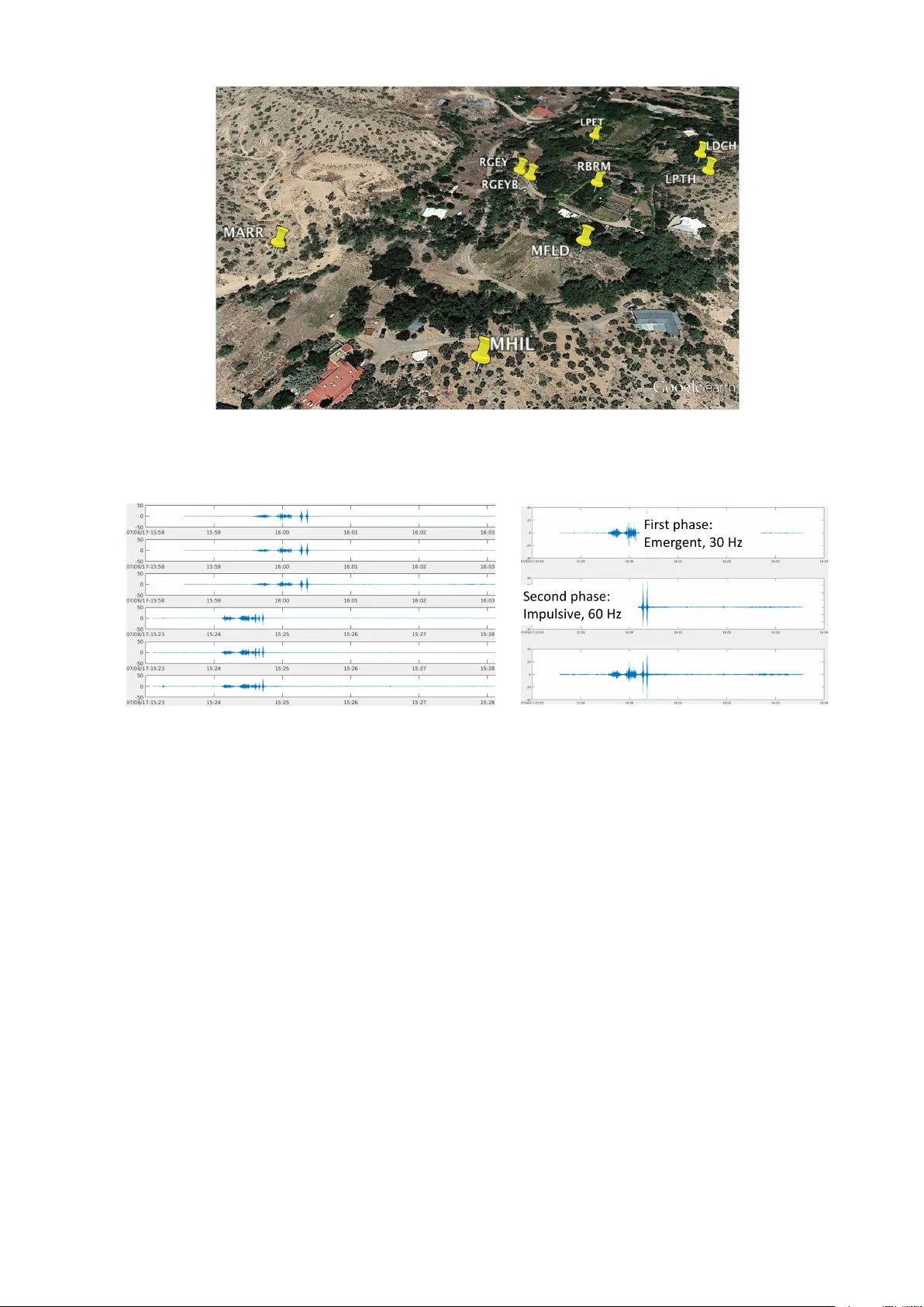
Seismic-Net: A Deep Densely Connected Neural Net w ork to Detect Seismic Ev en ts Y ue W u, Y ouzuo Lin, Zheng Zhou, and Andrew Delorey Earth and En vironmen t Sciences Division Los Alamos National Lab oratory Los Alamos, NM 87545 Abstract One of the risks of large-scale geologic carb on sequestration is the p o- ten tial migration of fluids out of the storage formations. Accurate and fast detection of this fluids migration is not only imp ortant but also c hallenging, due to the large subsurface uncertain ty and complex go v erning physics. T raditional leak age detection and monitoring tec h- niques rely on geoph ysical observ ations including seismic. How ever, the resulting accuracy of these metho ds is limited b ecause of indirect infor- mation they provide requiring exp ert in terpretation, therefore yielding in-accurate estimates of leak age rates and lo cations. In this work, we dev elop a no vel machine-learning detection pack age, named“Seismic- Net”, which is based on the deep densely connected neural netw ork. T o v alidate the p erformance of our proposed leak age detection metho d, w e employ our method to a natural analog site at Chimay´ o, New Mex- ico. The seismic ev ents in the data sets are generated b ecause of the eruptions of geysers, whic h is due to the leak age of CO 2 . In particular, w e demonstrate the efficacy of our Seismic-Net by formulating our de- tection problem as an even t detection problem with time series data. A fixed-length window is slid throughout the time series data and we build a deep densely connected netw ork to classify each window to de- termine if a geyser even t is included. Through our numerical tests, we sho w that our mo del achiev es precision/recall as high as 0.889/0.923. Therefore, our Seismic-Net has a great p otential for detection of CO 2 leak age. 1 In tro duction A critical issue for geologic carb on sequestration is the ability to detect the leak age of CO 2 . There has b een three ma jor different geophysical metho ds emplo y ed to detect the leak age of CO 2 : seismic metho ds, gra vimetry , and electrical/EM metho ds [1, 2]. Among those metho ds, the seismic metho d is presen tly without any doubt the most p ow erful metho d in terms of plume mapping, quantification of the injected v olume in the reservoir and early detection of leak age [1]. In this work, we employ seismic data to detect the leak age of the CO 2 . Copyright c  2016 by the p ap er’s authors. This volume is publishe d and c opyrighted by its e ditors. . In: A. Jorge, G. Larrazabal, P . Guillen, R.L. Lop es (eds.): Pro ceedings of the W orkshop on Data Mining for Oil and Gas (DM4OG), Houston, T exas, USA, April 2016, published at h ttp://ceur-ws.org 1 Figure 1: Map of Chimay´ o, New Mexico [4]. F aults are sho wn as red lines. The lo cation of the geyser is shown as red dot. The sedimentary basins of Chima y´ o, New Mexico hav e become prominent field lab oratories for CO 2 seques- tration analogue studies due to the naturally leaking CO 2 through faults, springs, and wellbores [3]. The site of Chima y´ o Geyser is lo cated in Chima y´ o, New Mexico within the Espanola Basin (Fig. 1). The b edro ck consists predominately of sandstones cut by north–south trending faults. Chimay´ o geyser lies near the Rob erts F ault and may cut directly through it. The source of CO 2 is unknown for the region. The regional aquifer supplying Chima y´ o geyser is semi-confined. The well was originally drilled in 1972 for residen tial w ater use but ended up tapping in to a CO 2 -ric h w ater source and has geysered ever since. It has a diameter of 0.10 m, depth of 85 m and is cased with PV C for the en tire depth. T o acquire seismic data, multiple stations are deploy ed at several p oints of in terest, contin uously recording time series signals as a time-amplitude representation. The lo cations of the seismic stations are shown in Fig. 2. The time series data has three comp onen ts, represen ting amplitudes of three p erpendicular directions. In this w ork, w e only use one comp onen t of the signals from one station. Figure 3a illustrates the signals of tw o geyser even ts. Eac h even t can b e separated into tw o phases– emer gent and Impulsive , whic h are shown in Fig. 3b. It is worth while to men tion that the n umber of amplitude p eaks in the second phase ma y b e arbitrary . Geyser ev ent detection from seismic data can b e formulated as even t detection problem with time series signals. Our main idea is to slide a fixed-length window through the time series data and use a binary classifier to detect whether there is a geyser ev ent within. T radition ev ent detection algorithms that are widely used in the geoph ysics communit y are mainly similarity-based [5, 6, 7]. These algorithms are extremely inefficien t (it takes w eeks to iterate ov er the whole time series data) and not very accurate. Thus, we aim at dev eloping machine learning mo dels to significan tly accelerate the inference pro cedure and b o ost the accuracy . Con v olutional neural netw orks (CNN) hav e demonstrated the great p oten tial to pro cess image data [8, 9]. It is natural to translate similar metho dology into our 1D time series scenarios. CNN is particularly p ow erful to capture target patterns. F or time series data, lo cal dynamics are captured b y shallow la yers of a CNN due to the lo cal connectivity . As the netw ork becomes deep er, longer-range dynamics can b e captured with the increasing size of the receptiv e field, that is, the pattern of the target wa v eform can b e captured with a deep CNN. The state-of-the-art CNN architectures hav e b een revolu tionized since He et al. [10, 11], known as ResNet where skip connections are built to mak e the netw ork substantially deep. The merit of skip connections can b e understo o d from tw o p ersp ectiv es. Firstly , they enable the gradient from the output la y er backpropagate directly to shallo w la y ers, alleviating the notorious gradien t v anishing problems [12]. Secondly , the whole arc hitecture can b e viewed as a h uge ensemble since there are numerous paths from the 2 Figure 2: The distribution of seismic stations. The lo cation of each seismic station is shown in yello w pin. (a) (b) Figure 3: (a): Time series signals of tw o geyser even ts, eac h with three p erp endicular channels. (b): An illustration of the tw o phases of a geyser even t. The first phase is called emer genc e with 30 Hz of frequency . The second phase is called impulsive with 60 Hz of frequency . input lay er to the output lay er, which significantly increases the robustness of the mo del and reduces ov erfitting. In this w ork, we built our model up on the densely connected block [13] (DenseNet), which is an impro v ed v ersion of ResNet. In a densely connected blo c k, the output of a conv olution lay er is densely c onne cte d with all previous outputs. The “connection” is implemented by concatenation op eration. Th us, it fully exploits the adv antage of the skip connection, while k eeping a reasonable n um b er of parameters through the reuse of features. In this w ork, w e explore the p otential of the densely connected netw ork in time series classification tasks. W e use geyser data collected by several stations to ev aluate our mo del. The exp erimen tal results show that our mo del can accurately detect geyser even ts without b ells and whistles, which suggests the p otential of the densely connected net w ork for addressing c hallenging time series tasks. 2 Prop osed Model: Seismic-Net In this section, w e describ e the structure of our Seismic-Net. 3 Stage La y e rs Dim. Input - 18000 × 1 Con v olution con v7, 24, /2 9000 × 24 P o ol a vg-p o ol2, /2 4500 × 24 D 1 [con v3, 12] × 6 4500 × 96 P o ol a vg-p o ol2, /2 2250 × 96 D 2 [con v3, 12] × 6 2250 × 168 P o ol a vg-p o ol2, /2 1125 × 168 D 3 [con v3, 12] × 6 1125 × 240 P o ol a vg-p o ol2, /2 563 × 240 D 4 [con v3, 12] × 6 563 × 312 P o ol a vg-p o ol2, /2 282 × 312 D 5 [con v3, 12] × 6 282 × 384 P o ol a vg-p o ol2, /2 141 × 384 D 6 [con v3, 12] × 6 141 × 456 P o ol a vg-p o ol2, /2 72 × 456 D 7 [con v3, 12] × 6 72 × 528 P o ol a vg-p o ol2, /2 36 × 528 D 8 [con v3, 12] × 6 36 × 600 P o ol a vg-p o ol2, /2 18 × 600 D 9 [con v3, 12] × 6 18 × 672 P o ol a vg-p o ol2, /2 9 × 672 D 10 [con v3, 12] × 6 9 × 744 P o ol a vg-p o ol9, 9 1 × 744 1-d fully connected, logistic loss T able 1: Net work architecture of our Seismic-Net. This mo del is designed for inputs with 18,000 timestamps, whic h is ideal to effectiv ely capture all geyser ev en ts. 2.1 Densely Connected Blo ck A densely connected blo c k is form ulated as x l +1 = H ([ x 0 , x 1 , ..., x l ]) (1) H ( x ) = W ∗ ( σ ( B ( x ))) , (2) where W is the w eight matrix, the operator of “*” denotes conv olution, B denotes batc h normalization (BN) [14], σ ( x ) = max(0 , x ) [15] and [ x 0 , x 1 , ..., x l ] denotes the concatenation of all outputs of previous lay ers. The feature dimension d l of x l is calculated as d l = d 0 + k · l, (3) where k, the gr owth r ate , is the n um b er of filters used for eac h conv olution lay er. 2.2 Net work Architecture T able 1 illustrates the o v e rall architecture of our netw ork. All conv olution kernels in our netw ork are 1 dimensional b ecause of the input of 1D time series data. Con v7, 64, /2 denotes using 64 1 × 7 conv olution kernels with stride 2. The same routine applies to p o oling lay ers. L denotes the length of input wa veform. The brack ets denote densely connected blo cks, formulated in Eq. (2). W e set the gro wth rate k = 12 for all densely connected blo cks, whic h results in 744 extracted features for one time series segment. All densely connected blo cks are follow ed by an av erage p o oling lay er, which downsamples the signals by 2. The last av erage p o oling lay er a verages features o v er all timestamps to capture global dynamics. The global av erage p o oling la yer is follo wed b y a fully connected la y er, whic h is implemented as x ( l +1) = W · x ( l ) + b, (4) where W is the w eigh t matrix and b is the bias. W e use logistic loss as the loss function, which has the form LL( y , z ) = log(1 + e − y z ) , (5) 4 Figure 4: A segment of our geyser data. A geyser even t is in the window indicated by a green dot and red cross. where y ∈ {− 1 , 1 } is the ground-truth, z is the predicted score. In the inference stage, the predicted label is based on the sign of the score. This architecture is designed for inputs that hav e 18,000 timestamps ( L = 18 , 000). This size of input signal is carefully c hosen to effectiv ely co v er all geyser ev en ts. 3 Implemen tation Details In the training stage, we take 18,000-timestamp segm en ts with geyser even t included as positive samples. Neg- ativ e samples includes manually pick ed 83 segments and 330 randomly pick ed segments from non-ev ent signals. Since we only hav e the geyser even t annotated, we found that man ually picking most representativ e negative ev en ts necessary to achiev e a go o d p erformance. W e pre-pro cess the time series data by substracting the mean, then dividing the standard deviation. W e use Adam optimizer [16], a v ariant of sto chastic gradien t descent algo- rithm, to minimize the loss function. W e set the batch size to 50. The total num b er of parameters of our mo del is approximately 800K. It tak es roughly 50 epo chs to conv erge. Our mo del is implemented in T ensorFlow [17]. W e trained our mo del on a single NVIDIA GTX 1080 GPU. T o test our mo del, w e feed 18,000-time stamp windo ws in to the mo del with 6,000-timestamp offset. W e store the score of each p ositive detections. F or multi-detections of the same ev en t, we only keep the one with the highest score and discard the rest. 4 Exp erimen tal Results 4.1 Seismic Data W e deploy multiple stations to contin uously recording time series signals near the p oint of interests. The distribution of the stations are shown in Fig. 2. In this w ork, we only use signals from RGEYB to train and test our mo del. W e hav e lab eled signals in 55 days. Signals from 23 days, including 33 even ts, are used for training. Signals from 32 days, including 26 even ts, are used for testing. A day-long data has 17,280,001 timestamps. Geyser eruption happ ens at most twice a da y . The longest geyser even t in our dataset spans 12,000 timetamps. Figure 4 giv es an illustration of a segmen t of our data with a geyser even t included. The even t happ ens within the window bounded by a green dot and a red cross. All other signals are considered noise. As previously men tioned, some negativ e samples are hand-pick ed due to the unknown negative sample space. Some negative samples include eruptions caused by passing trains and h uman activities, whic h may fo ol the classifier if not included in the training set. 4.2 Results The detection results w.r.t. several different metho ds are provided in T able 2. W e compare the p erformances of four mo dels: 1) supp ort v ector machine with radial basis function kernel; 2) VGG-based [9] CNN; 3) ResNet- based CNN and 4) DenseNet-based CNN. W e use the same training routine as the prop osed CNN to train the k ernel SVM. W e found that the kernel SVM has extremely low accuracy so we put “fail” in the table. It suggests that adv anced feature extraction tec hniques are required in adv ance to apply SVM, logistic regression or other shallo w mo dels. 5 Precision Recall # P arameters Kernel SVM fail fail 18K V GG-based Net 0.609 0.538 37M ResNet-based Net 0.581 0.960 15M Seismic-Net 0.889 0.923 800K T able 2: The detection results given b y kernel SVM, CNN inspired b y V GG net, ResNet-based CNN and densely connected CNN. “fail” indicates extremely low accuracy . These results indicates that the shallow mo del (SVM) is greatly outp erformed by deep mo dels. The densely connected netw ork stands out among other CNN-based mo dels. The V GG-like net work has no skip connections, whic h is the ma jor difference with ResNet-based or DenseNet- based netw ork. Since the input size is large (18,000 timestamps), more conv olution lay ers are required to capture the global dynamics, which makes the num b er of parameters in VGG-based net work substantially . The optimization for VGG-based net w ork is rather difficult without the help of skip connections. Thus, it has the lo w est accuracy among the three CNN-based mo dels. The ResNet-based mo del, with skip connections, has the second best p erformance. The DenseNet-based mo del, with densely connected conv olution lay ers, has the b est p erformance. It has 24 correct detections (TP) out of 27 (TP + FP) total detections. The num b er of ev en ts in test set is 26 (TP + FN). W e use precision and recall as the ev aluation metrics. They are calculated as Precision = TP TP + FP , (6) Recall = TP TP + FN , (7) where TP stands for “true p ositiv e”, FP stands for “false p ositiv e” and FN stands for “false negativ e”. 5 Example Detections (a) (b) (c) (d) Figure 5: Some example detections are shown here. These four even ts demonstrate that our mo del is able to accurately detect geyser even ts even though the patterns are not alw ays similar since the n um b er of eruptions in the t wo phases is arbitrary . The green dot and the red cross indicate the location of the sliding windo w where our mo del giv es p ositiv e predictions. 6 W e present four detections giv en b y our mo del in Fig 5. These results indicate the p otential of our mo del to accurately capture sp ecific patterns in time series signals. Although the patterns of geyser even ts v ary , which is caused by the arbitrary num b er of eruptions in the second phase, those even ts are still correctly detected b y our DenseNet-based CNN. The wa veforms of the second phase are those “thinner” eruptions. Fig. 5 (a), Fig. 5 (b), Fig. 5 (c), and Fig. 5 (d) hav e 2, 2, 4 and 1 amplitude p eaks in the second eruption, resp ectively . The lo cations of the triggered sliding windo w is indicated b y a green dot and a red cross. 6 Conclusion In this work, we developed a seismic even t detection pack age, entitled “Seismic-Net”. Our Seismic-Net is based on conv olutional neural netw ork and is capable of detecting seismic ev ents accurately and efficiently . Our net work is substan tially deep in order to capture global dynamics. Densely connected blo cks are inserted to reduce the n um b er of parameters and simplify the optimization. W e employ our Seismic-Net to a natural analog site at Chima y´ o, New Mexico. The exp eriment results demonstrate that our model achiev es high accuracy without b ells and whistles. By comparing with shallo w mo dels and other con volutional neural net w ork v ariants, we justify that the proposed DenseNet-based architecture is the most accurate mo del. It is also the most efficient among conv olutional neural netw ork-based mo dels with only 800K parameters. Th us, we conclude the prop osed mo del has a great p otential capture complicated patterns in time series data, therefore can b e used for an early detection of CO 2 leak age. Ac knowledgmen t This work was co-funded by the Center for Space and Earth Science at Los Alamos National Lab oratory , and the U.S. DOE Office of F ossil Energy through its Carb on Storage Program. References [1] H. F abriol, A. Bitri, B. Bourgeois, M. Delatre, J. Girard, G. Pa jot, and J. Rohmer, “Geophysical metho ds for co2 plume imaging: comparison of p erformances,” Ener gy Pr o c e dia , v ol. 4, pp. 3604–3611, 2011. [2] A. Korre, C. E. Imrie, F. May , S. E. Beaubien, V. V andermeijer, S. P ersoglia, L. Golmen, H. F abriol, and T. Dixon, “Quantification techniques for p oten tial co2 leak age from geological storage sites,” Ener gy Pr o c e dia , vol. 4, pp. 3413–3420, 2011. [3] M. Han, W. S. Lu, B. J. McPherson, E. H. Keating, J. Mo ore, E. Park, Z. T. W atson, and N. Jung, “Char- acteristics of co2-driven cold-water geyser, crystal geyser in utah: exp erimental observ ation and mechanism analyses,” Ge ofluids , vol. 13, pp. 283–297, 2013. [4] Z. W atson, W. S. Han, E. H. Keating, N. Jung, and M. Lu, “Eruption dynamics of co2-driven cold-water geysers: Crystal, tenmile geysers in utah and chima y´ o geyser in new mexico,” Earth and Planetary Scienc e L etters , v ol. 408, pp. 272–284, 2014. [5] S. J. Gibb ons and F. Ringdal, “The detection of low magnitude seismic even ts using arra y-based wa veform correlation,” Ge ophysic al Journal International , vol. 165, pp. 149–166, 2006. [6] J. R. Brown, G. C. Beroza, and D. R. Shelly , “An auto correlation metho d to detect low frequency earth- quak es within tremor,” Ge ophysic al R ese ar ch L etters , v ol. 35, no. 16, p. L16305, 2008. [7] C. Y oon, O. O’Reilly , K. Bergen, and G. Beroza, “Earthquake detection through computationally efficien t similarit y searc h,” Scienc e A dvanc es , v ol. 1, no. 11, pp. 1–13, 2015. [8] A. Krizhevsky , I. Sutsk ever, and G. E. Hin ton, “Imagenet classification with deep con volutional neural net w orks,” in NIPS , 2012, pp. 1097–1105. [9] K. Simony an and A. Zisserman, “V ery dee p con v olutional netw orks for large-scale image recognition,” in ICLR , 2015. [10] K. He, X. Zhang, S. Ren, and J. Sun, “Deep residual learning for image recognition,” in CVPR , 2015. [11] ——, “den tit y mappings in deep residual net w orks,” in arXiv pr eprint arXiv:1603.05027 , 2016. 7 [12] Y. LeCun, B. Boser, D. J. S., D. Henderson, R. E. How ard, W. Hubbard, and L. D. Jac k el, “Backpropagation applied to hand- written zip co de recognition,” Neur al c omputation , vol. 1, pp. 541–551, 1989. [13] G. Huang, Z. Liu, and L. v. d. Maaten, “Densely connected conv olutional netw orks,” in CVPR , 2017. [14] S. Ioffe and C. Szegedy , “Batc h normalization: Accelerating deep net work training by reducing internal co v ariate shift,” in ICML , 2015. [15] V. Nair and G. E. Hinton, “Rectified linear units impro v e restricted Boltzmann machines,” in ICML , 2010. [16] D. P . Kingma, , and J. Ba, “Adam: A metho d for sto chastic optimization,” in ICLR , 2014. [17] M. Abadi, A. Agarwal, P . Barham, E. Brevdo, and Z. Chen, “T ensorflo w: Large-scale machine learning on heterogeneous distributed systems,” in , 2016. 8