Multilateration of the Local Position Measurement

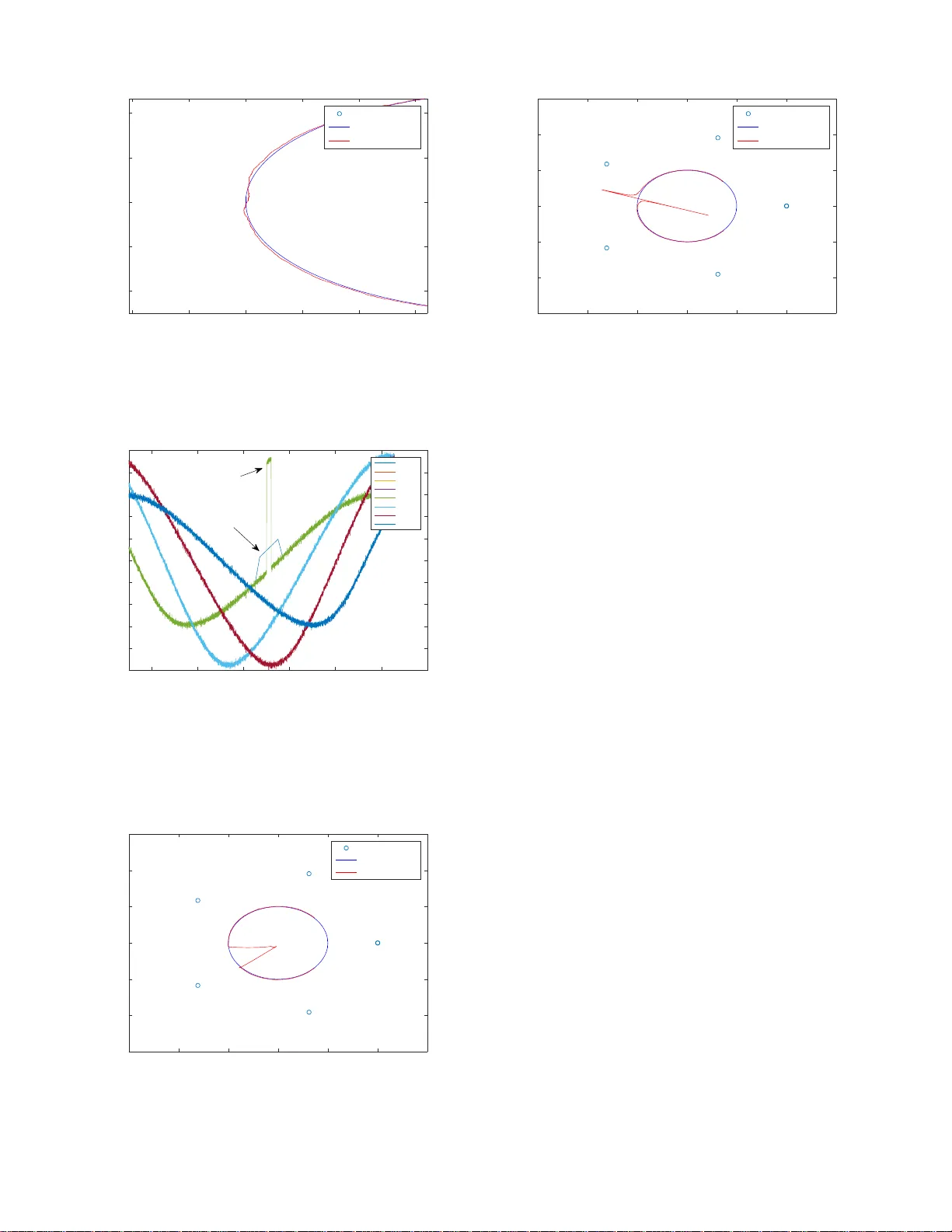
Multilat eration of the Lo cal Po s ition Measurement Juri Sidorenko, Norbert Scherer -Negenborn, M ichael Arens, Eckart Michaelsen Fraunho fer Institute of Optronics, S ystem T echnolo g ies and Image Exploitation I OSB Gutleuthausstrasse 1, 76275 Ettlingen, Germ a ny . Juri.Sidoren ko@iosb .fraunhofer .de Abstract —The Local Position Measurement system (LPM) is one of the most precise systems for 3D position estimation. It is able to operate in- and outdoor and updates at a rate up to 1000 measurements p er second. Previous scientific pub lications fo cused on th e time of arriva l equation (TO A) pro vided by the LPM and fi ltering after the numerical position e stimation. This paper in vestiga tes the adv antages of the T O A o ver the time difference of arriv al equ ation transfo rmation (TDOA) and the signal s moothing prior to i ts fittin g. The LPM was designed under the general assumption that the position of the base station and position of the refer ence station are known. The information resulting from this r esearc h can prov e vital for the system’ s self- calibration, providing data aiding in locating the relativ e position of the base station without prior kno wledge of the transponder and reference station positions. Key words: time of arrival, time difference of arrival, local position me asurement I . I N T R O D U C T I O N In the past, a wide range of different methods and sensors have been developed to o b tain th e exact position of an object of interest. The most common are ra dio frequency based methods, like N A VSA T GPS. This technolo gy is often used as an e xample for the time of arriv al equ ation (TO A). The tr aveling time between the satellite and the sensor on the ground c a n b e used to estimate the sen sor’ s position, neglecting the p osition estimation by phase. Both, the satellite’ s position in its or b it and the signal’ s send tim e , are k n own. Combining this in formation with th e time sign al arriv al on the groun d an d the speed of light, it is th en possible to estimate th e range between the satellite and the sensor . This range is called pseud o ran ge. If we neglect the time offset, thr ee satellites are required to estimate the sensor’ s 3D position. Unfortu n ately , th e data update is quite slow a nd un su itable for urban territo ry . Dur ing WWII, TDOA sy stem s like DECCA became very popu lar . T he T DO A me thod does no t req uire knowledge o f emission time s. In contrast to the TOA, all possible locations f or one mea su rement are located on a hyperb ola. Other method s, like the angle o f arriv al, will not be addressed in this paper . All examples used from here on out will be based on th e Abatec LPM. This system has potential, due to the fact that it is ab le to operate both in- and outdoo rs a n d p rovide an update rate of 1000 measuremen ts per second. f 1( T1 ) f2 ( T2 ) D f ( T ) Time f(T1) Send f(T2) Recived f2(T2) Intern Send Recive K f3(T2) Basissation (BS) Intern Fig. 1. FMCW: Left increa sing freque ncy chirp with slope K. Right: mixed frequenc ies MT Bs 1 f ( T ) Time Bs 2 RT Offset RT_BS 2 Offset MT_BS 2 BS 1 BS 2 MT RT ||MT -BSn|| - ||RT -BSn|| - Offset_MT_RT = PRn Lateration Fig. 2. LPM Left: Offset differen ce betwe en transponder MT , basis s tation BS and reference stat ion R T . Right: L PM euclidi an equation The LPM was hig hly inspired b y the FMCW fre quency modulated continues wave radar (FMCW) and systems based on TO A, such as GPS. Fig ure 1 illu strates the f unctionality of a FMCW . The internal system is gener a ting an increasing frequen cy chirp with a fixed slop e K. This chirp is sent and reflected by an o bject. The re ceiv ed signal does no t change its freq uency , but dur in g this time ( T 2 − T 1) the internal frequency ch a n ged from f 1 to f 2 . The radar can use an add iti ve or multiplicative m ixer to obtain the sum of the two freq uencies an d th eir differences. As o nly the frequen cy difference is required at this po in t, the frequency sum can b e filtered by a low pass filter . The LPM is using this pr inciple alread y , but in contrast to the FMCW radar , the send freq uency ch irp is getting compar e d with the frequency chirp o f the other base station K B S 1 = K B S 2 (fig ure 2). If the chirp s a r e synchro nized (started at the s ame time) th ere is no offset, b ut since the base station s an d transpo nder are not synchro n ized, a refer ence station is r equired. Every fr equency measuremen t the LPM provides is based on the difference between the tran sponder an d o ne o f the base stations with respect to the referen ce st ation at the same ba se station. Due to this fact, the tim e offset O is eq ual f o r every base station for the same measurement as demonstra ted in fig. 2. Th is all leads to the LPM equatio n (1), with R: Pseud o Range, O: Offset, M: T ransponder- an d T: Refe r ence station for different measuremen ts i. R i = O + k M − B i k − k T − B i k (1) k M − B i k = q ( x i − x M ) 2 + ( y i − y M ) 2 (2) k T − B i k = q ( x i − x T ) 2 + ( y i − y T ) 2 (3) I I . P R E V I O U S W O R K The measurem ent pr in cipal of th e Ab atec L PM and its hardware implemen tation ha ve been pr esented in [ 6] [9]. Pre- viously published work abou t the LPM predomin antly focused on the usage of Kalman filters to d e tect an outlier[3] or to track the p osition of the tran sponder [7]. An approac h to o u tlier detection can be found in [3], were the linear Kalman filter in co mbination with the χ 2 test was used to de tec t outlier s within the offset corrupted data. No nlinear equatio n solving with Bancroft is analy zed in [8][11] and co mpared with the least median of squ ares (LMS) in [2]. Abatec LPM (state-of-the-art): • Solving of no n linear TO A equation with a num erical solver . • Unknown variables are co ordinates of the transp o nder and the of fset. • Filtering after no nlinear multilateration. New a ppr oach: • TO A to TDO A transformation. • The TDO A data is filtered before the multilateration . • Both a lin ear TDO A solution and a nonlinear TDO A solution may be u sed to filter data before the lateration. Advantages o f ne w appr o ach: • Filtering before solving has the adv antage that Gau ssian noise inside of measurem e n t data does n ot ch ange du e to numerical solver . • The linear solu tio n is faster than the nonlinear so lu tion. • The nonlinear so lution does not have to fit the of fset. • W ith o ut the offset, outlier detection is enab led. Disadvantage of new appr oach: • The TDO A solution requires an a dditional base st ation • The linear solu tio n is mo re easily affected by un fa v orable condition s . I I I . M E T H O D O L O G Y The pr e vious section in troduced the LPM and th e following focuses on its position estimatio n . In general, the exact posi- tions of the reference station an d base s tations are known. In this way , fo ur base stations are r equired to obtain the x, y , an d z coord inates of the transp onder . The euclidean form for this equation can be solved u sin g eithe r the Gauss-Newton m ethod, or an other non-linear solver . Altern ati vely , the equa tio n may be linearized with a T aylor-series expansion [4] within a starting position. Unf ortunately , in that case, the solu tion dep ends heavily on a go o d estimation of th e starting conditio n . In order to detect the outlier and to ob tain a s trong starting conditio n s, one need s to analyze the da ta. The gener a l appr oach for the LPM to detec t an outlier was using Chi-test within a linear Kalman filter (LKF) [3] on raw data. Figure 3 sho ws tha t the offset ( O ) is 1 0 6 times highe r than the mea su rement itself. Furthermo re, the offset is changing from o ne measur e m ent to the n ext, due to the difference in oscillator clocks of reference station and transpo nder [3].Th e elimination o f the offset allows us to s ee the relati ve r ange chang in g b etween the tr anspond e r and base station. Th is can b e done by subtracting on e base station from another at the same measur ement. In fig ure 4 the result of this tran sformation on real measurem ents can be seen. The ou tliers ar e now visible with th eir typical c haracteristic of reflected data. At this point the TOA eq uation is changing to the TDO A. In [1 0] it was proven that the error propag ation of the TDOA is equal to tha t of the TOA. Th is transformatio n can be done for two p urposes: first, on e may ob tain the relative range between th e base station and eliminate the offset; in this way we are able to filter data a nd o utliers; second, on e can rearrange the T O A equ ation to g et the lin ear form of the transpond er x, y , and z coordinates. Fig. 3. LPM real raw data with offset Z at differ ent measure ments 0 5 10 15 Samples × 10 4 -10 -5 0 5 10 (PRm-PRn) [m] Fig. 4. Pseudo range of the real data after the transformation TO A to TDO A A. Line a rization Approac h es such as th e T aylor-series expansion [4] or oth er nonlinear solvers can b e used to linearize the (1) equation s. These method s req u ire start in formation for the u nknown variables. A lter nativ ely one may use a ref erence station to obtain linear terms for th e unknown p osition o f th e transpon - der . The o ffset will still be a part of the equation, but, just like the coo r dinates o f the transp o nder, will b e linear . This technique is also known as linea r least square s multilateration. The main LPM equation (1) c a n be simplified by add ing the known referen c e transponder ran ge to th e measuremen t term R (pseudo range). L i = R i + k T − B i k (4) k M − B j k 2 − k M − B i k 2 = ( L j − O ) 2 − ( L i − O ) 2 (5) The known quad ratic ter m s o f th e tra n sponder are elimi- nated, h ence the linear solution for the transpond er position at the known base station and reference station position is:  − → B i − − → B j  · − → M − ( L i − L j ) · O = = 1 2   − → B i  2 −  − → B j  2  −  L 2 i − L 2 j   (6) with − → M =  x M y M  − → B =  x B y B  The state-of -the-art Abatec L PM software u ses a da mped Newton iteration for nonlin ear regression [1 1], requir ing som e start positions ar e req uired. The solution here p resented, does n ot req uire any start po sition or n onlinear so lvers. Th e method’ s result, howev er , depend s on the condition of the coefficient ma tr ix (A). Should the piv ots ( diagonal elements of the coefficient matrix) b e close to zero the condition is bad. B. Fil tering The transfo rmation of the TOA to TDO A by sub tracting one base station fr om a re f erence station can also be used to filter data. If equatio n 1 is not getting solved for T and squ ared before subtra cted from a ref erence station, the term will still be non linear for th e unknown position of the transpon der, but the of fset wil l be eliminated. As mentioned above, e very mea su rement has its offset, wh ich is usually 10 6 times higher than the location itself. If th e numerical solver do es not take this into account and the start condition s for the offset are unfav orable, then the chan ging in x, y , and z co ordinates have almost n o effect on the residuals. The higher the difference between || M − B || and offset O the higher th e d eviation between lo cal optima an d glo b al op timum. Another p roblem could appear R + || T – B || > O in this case, the minimum of the numerical optimizatio n b ecomes the maximu m. T he most suitable starting value for the offset would be the mean for every measu rement, but we are still not able to set any start condition for th e coordin ates of the transpond er or to interp ret th e measure m ents. In addition , the offset is c h anging from one measureme n t to the next, hence it prom ises suitable to u se the difference between the base stations with resp ect to one r eference station for th e same measurem ent f or fur ther calculations. This method is known as the hy perbolic meth od [8] , due to th e fact that the pseudora n ge is no t main tained fro m the perspective of the transpond er , if moving with a fixed radius o n a circle ar o und the b asisstion, but in order to maintain the same pseudorang e movement has to rem ain on a hyp erbola. Changin g the base station’ s instead the o f tr a nsponder ’ s position would provid e a hyperb olic shap e from the beginn ing. T his shap e is typical for TDO A, h owe ver , now the multidimen sional damp e d Newton is utilized to solve the m inimization of the equ ation [ 11]. Data may be filtered before position estimation, without the offset. The g eneral approach for the LPM was to use the extended Kalman Filter, (E K F) [7] on the data provided by the numer ical solver . But e ven if the d ata of the measuremen ts h a s a gaussian noise, it does not nece ssarily mean that numerical ou tput h as a gaussian distribution as well. The least squares method to minimize the residuals mi n n P i =1 1 2 ( f ( x, y , z ) − y i ) 2 is e ffected by ou tliers, but is able to deal with g a u ssian noise. A bad matrix condition o r po o rly cho sen starting con dition cou ld lead to a result, which do es n ot have a gaussian d istribution anymore and therefo r e ma kes filterin g the da ta before solv ing an ad vantage accompanied by a solver that d oes no t have to estimate the offset. The solver conver ges faster and filtering can be one dimensiona l instead of three dimen sional. T he difference between th e base station s to one ref erence station causes a de pendency betwee n th e equatio n s due to n oise [1]. Based o n empir ica l measuremen ts, the variance of the noise ( figure 5) f or every b ase station differs f rom 0 . 003 m 2 to 0 . 00 36 m 2 for an immo bile transpon d er . Th us one can assume that the v ariance is equ al for every base station. This is an impo rtant fact for itera tive solving. The r e are sev eral filters ap plicable to filterin g the data in qu estion. A very y( BS 1 - BS 3) 1.45 1.5 1.55 1.6 1.65 1.7 1.75 1.8 1.85 1.9 Number of measurements 0 50 100 150 200 250 300 Mean: 1.6675 Variance: 0.003 Fig. 5. B S 1 − 3 , Real d ata based gaussian di strib ution of the pseudo range dif ferenc e for a not m ovin g tran sponder fast and simple filter is the m ovin g average filter . This filter proves h e lpful when the f ocus lies on the time domain instead of the freq uency d omain. I ts filter kernel (imp ulse resp onse of the filter) do es n ot requ ire a con volution with a signal, instead, pr ocessing can be red uced to subtracting th e oldest measuremen t and addin g one of the latest measureme nts. Due to the central limit the o rem, runn ing th e filter several times would lead to a similar re su lt as using a c o n volution with a gaussian kernel. In this way th e over and un der oscillations of the frequ ency domain are redu ced. The me thod is faster than the conv olution with a Gaussian kern el. In figure 6 the result of the moving a verage fi lter , which is a Finite Impulse Response filter (FIR) illustrating the moving variance o n real data after the transformation . All outliers have a high v ariance with respect to the other measuremen ts. This inf ormation can be used no t just to detect the tr a nsponder, but also the source of the re flec tion. Th e disadvantage of this method is a delay ( N − 1) / 2 , which is increasing with the numb er of sam ples N . As an alternati ve, one co u ld use the linear one dimen sional Kalman filter instead . The d ifference b etween TO A an d TD OA is visible ( fig.7) Green circles represent the probab ility of the transpon der location . Every circle represen ts one euclidean equation at a certain measure m ent. The correct location fits all th e equations, th erefore the residu als a re the smallest. Smaller resid u als are pro duced where just two equations fit, compa red to othe r position s, hen ce the f ound coordin ates a r e th e local o ptimum (L O). Th e transfo rmation results in simplified, hyper bola and triangles. T he position of the transponder can be foun d by two hyperbola, but thr e e hyperb ola can be p roduce d . The thir d can be represen ted by the oth er two, this hy p erbola has n o fur ther informa tio n compare d to th e other two, but dif ferent local optima and another intersection ang le. Due to this fact, n umerical solving may influen ce, just b y tra nsforming , the pro bability to find a local optimu m . 0 2 4 6 8 10 12 14 Samples × 10 4 -10 0 10 20 30 40 50 PR (BS1-BS2) [m] FIR Variance Fig. 6. Example of reflect ion inside real data. Red curve represents v arian ce, blue measurements and the green the filtered data -5 0 5 10 15 X-Axis [m] -10 -5 0 5 10 15 Y-Axis [m] BS 3 BS 1 BS 2 RT MT L. O L. O L. O BS || 1 - 2 || BS || 1 - 3 || BS || 2 - 3 || Fig. 7. Dif ference betwe en TO A and TDOA . The triangl es are the simplifie d hyperbol oids of TDOA and the gree n circ les the eucl idean form of TOA Combination of the lin ear equatio n with filtered data The linear equation has some advantages over th e nonlin ear solution. Th is section presents a method of pr e-filtering, which can be used to c orrect the linear solu tion. T ests showed tha t the noise is ten time s higher than an im m obile transpon der , possibly due to the Dopp ler effect an d the micro movemen ts of the carrier . Therefo re, we increased the random n oise u p to a maximu m value of 0 . 1 m . The mean erro r of the estimated path with r espect to the real p a th is 0 . 506 m (fig. 8). The measuremen t L1 c a nnot be filtered as th e time offset ch ange with r espect to time is 10 6 times hig her than the rang e chang e itself. Th erefore, the offset is eliminated by su b tracting one base station measuremen t from the oth er ( L i − L j ) . In the next step this data is filtere d over time. At this point it does not matter what kind of filter is used, it is on ly impor tant that filterin g takes plac e before position estimation and that the filter u ses the m easurement difference ( L i − L j ) as an input. For the fo llowing calculations we on ly assum e that for -15 -10 -5 0 5 10 15 X-Axis [m] -15 -10 -5 0 5 10 15 Y-Axis [m] Basisstations Real path Estimated path BS 1 BS 2 BS 3 BS 4 BS 5 Fig. 8. Syntheti c data: Real pat h of t ransponder is located around the reference station with a radius of 5 m. The base station s have a distance of 10 m from the cente r and same distance to each other . Measurement data is corrpute d by gaussian noise. ev ery measur ement we already have difference ( L i − L j ) the filtered values F ( L i − L j ) the main a im is to use the filtered values instead of the measurement differences between th e base stations. Th e ( L 2 i − L 2 j ) term is n onlinear but the filtered values consist of the linear difference betwe e n the measuremen t ranges. One solution to using the filtered values would be to make every b ase station de p endent on th e same measuremen t erro r term α i . Every measuremen t is corr upted by th e measurem ent error α i, hen ce the real me a surement can be written as L = ˜ L + α . The co nnection between the measuremen t erro rs α i an d α j can b e f ound if the unfiltered measuremen t difference ( L i + α i ) − ( L j + α j ) is subtracted from the filtered values F ( L i − L j ) . F ij =  ˜ L i + α i  −  ˜ L j + α j  − F ( L i − L j ) (7)  ˜ L i − ˜ L j  ≈ F ( L i − L j ) (8) The assumption that the noise can b e neglected after the filtering, this leads to th e term F ij being the difference between the noises o f both signals. F ij = α i − α j (9) α j = − F ij + α i (10) The measur ement error is replac e d by eq. 1 0.  − → B i − − → B j  · − → M −  ˜ L i − ˜ L j + F ij  · O = = 1 2  − → B i 2 − − → B j 2 − ˜ L i 2 − ˜ L j 2 − F 2 ij + +2 · α k  ˜ L i − ˜ L j + F ij  It can b e observed that the time offset O , d epends on the same param e ters as the m easurement erro r  − → B i − − → B j  · − → M −  ˜ L i − ˜ L j + F ij  · ( O + α k ) = = 1 2  − → B i 2 − − → B j 2 − ˜ L i 2 − ˜ L j 2 − F 2 ij  W ith at least fou r base statio n s, the un known co ordinates of th e tran sp onder can be estimated. W ith the filtered values the linear direct solutio n provides better results, than with the unfiltered equ a tion Ax = b . Th is equa tio n can be solved as:   x M y M O   =  A T A  − 1 A T b Figure 9 presents the resu lts of the new equation with n o ise. The m ean er r or with a perfect filter is now b elow 1 0 − 11 m . The experiment was repea ted with sy n thetic data and a real moving average filter to investigate th e b ehavior of outlier s. Simulating a seco nd base reflection the sample was set from 3500 to 360 0 an outlier o f 10 me ters. -15 -10 -5 0 5 10 15 X-Axis [m] -15 -10 -5 0 5 10 15 Y-Axis [m] Basisstations Real path Estimated path BS 5 BS 3 BS 1 BS 4 BS 2 Fig. 9. Noise correcti on 5000 5100 5200 5300 5400 5500 5600 5700 Samples 2 2.5 3 3.5 4 4.5 5 5.5 6 6.5 7 Y-Axis [m] PR1 PR2 PR3 F(PR1) F(PR2) F(PR3) Fig. 10. Synthe tic data (PR) with gaussian noise and moving a vera ge filter F(PR) -7 -6 -5 -4 -3 -2 X-Axis [m] -4 -2 0 2 4 Y-Axis [m] Basisstations Real path Estimated path Fig. 13. Result of the weighting on synthet ic data with outlie r 1000 2000 3000 4000 5000 6000 7000 Samples -10 -8 -6 -4 -2 0 2 4 6 8 10 PR, F(PR) [m] F(PR1) F(PR2) F(PR3) F(PR4) PR1 PR2 PR3 PR4 Outlier PR1 Outlier F(PR1) Fig. 11. Filter error due to outlier : Such measurements are typical for signal reflecti ons -15 -10 -5 0 5 10 15 X-Axis [m] -15 -10 -5 0 5 10 15 Y-Axis [m] Basisstations Real path Estimated path BS 3 BS 2 BS 1 BS 5 BS 4 Fig. 12. Outlier position estimatio n -15 -10 -5 0 5 10 15 X-Axis [m] -15 -10 -5 0 5 10 15 Y-Axis [m] Basisstations Real path Estimated path BS 3 BS 2 BS 1 BS 5 BS 4 Fig. 14. Result of weight ing at unfa v orable geometric condi tion Figure 11 shows th e results of the transformed sign al an d the filtered one ( figure 10). Th e outlier causes som e d isturbance in the filtered outp ut, wh ich leads to an e rror in th e po sition estimation (figu re 12). T his filter erro r can be min imized by taking variance into a c count. It is imp o rtant to remem ber that the d elay of the FIR filter to the sign al is ( N − 1) / 2 an d of the moving variance ( N − 1) / 2 p lu s th e delay of the FIR, therefor e we need som e samples for th e in itialization and have no position estimation a t the beginnin g ( fig . 12). The provided variance is now used to o btain the w e ig hting vector w = 1 /v ar .    w 1 . . . w n    Ax =    w 1 . . . w n    b The result of the weigh ting is visible in figu re 13, the mea- surement with the hig hest erro r now has the smallest we ight in the m inimizing of the least squ ares p roblem. That bein g said, in applyin g a working filter eliminates th e need for weights. Applying weighting at the po sition where the equ ation is sen- siti ve to pertur b ations like ( P R m − P R n + RT m − RT n ) ≈ 0 or B x , B y , B z ≈ 0 th e r esult of th e position estimation will be highly inaccu rate, due to cor r uption of the statistical meanin g (fig. 14). In con clusion, we nee d to compar e the n o nlinear and the lin ear solu tion. Both metho ds have b een tr ansformed and filtered b efore the late r ation. As a no nlinear solver we have used a Le venberg Marquard t method ( L VM) [5]. The starting conditio n for the solver was the result of th e pr evious fit beginning from the starting con d ition x, y, z = 0 and fit parameter (table I). Due to the TO A to TDO A equation transform ation, th ere is no nee d to fit the o ffset, fo r every step L VM x, y , and z co ordinates of th e tran sponder n eed to be estimated. -20 -10 0 10 20 X-Axis [m] -10 -8 -6 -4 -2 0 2 4 6 8 Y-Axis [m] Real path Linear Nonlinear Basisstations BS 2 BS 1 BS 6 BS 5 BS 3 BS 4 Fig. 15. L inear and Nonlinear T ABLE I N E W L I N E A R PA R A M E T E R Parame ter V alu e Scaled gradient 0.000001 Relat i ve funct ion impro vement 0.00001 Scaled step 0.001 Maximum iterati ons 20 Figure 15 pr esents th e results of bo th method s. The linear solution has a slightly highe r er ror rate co mpared to the nonlinear solution in some positions. The linear calcu lation, howe ver , too k 25 96 ms versus the nonlinear’ s 4 677 ms on a i7-4600 u CPU 2.10GHz and 16 GB Ram. It f ollows that if p r efiltering would be a ‘perfect’ approach , bo th solutions would have the sam e result a s th e real p ath. I V . C O N C L U S I O N S The transform ation f rom th e TO A e quation to the TDOA brings se veral ad vantages for th e L PM. Section 3 demonstrated that the transfor mation leads to a linear eq u ation, wh ich can be solved without initialization and numerical itera tio ns. Admittedly , th e linear solution as comp ared to the nonlin- ear TDO A solution is mor e sensitive to pertu rbations given specific geometric settings. Obtainin g the co ndition of the coefficient m atrix, thou gh, allows detection of these setting s, and permitting use of the faster linear solu tion for e very o ther position. The latter p art of section 3 d ealt with the TO A to TDO A transfo rmation with the aim to elimin ate the offset and to filter the data b efore the multilateration . Filtering the d ata before the po sition estimation, beca u se non-linear function estimation leads to violation of normal distribution, made more sense, howe ver . Furtherm ore, the transform a tio n allowed the detection of ou tliers, reducin g the number o f local optima and decreasing the compu tational time du e to th e elimination of the offset. I n the e nd, the line a r solution was expand ed with the p ossibility to use pre- filtered d ata and pr ovide a solu tion at in half th e time th at a non- linear solution can . R E F E R E N C E S [1] L ukasz Zwirello et al. Uwb localiza tion s ystem for indoor appli catio ns: Concept , realizati on and analysis,. In J ournal of Electrical and Com- puter Engineering , 2012. [2] Pfeil R et al. A robust position estimatio n algorithm for a local positioni ng measurement system. In W irele ss Sensing, Local P ositioni ng, and RF ID, 2009. IMWS 2009. IEEE MTT -S Internati onal Micr owave W orkshop on , pages 1–4, Sept 2009. [3] R. Pfeil et al. Distrib uted fault detect ion for precise and robust local positioni ng. In In Pr oceedi ngs of the 13th IAIN W orld Congr ess and Exhibiti on , 2009. [4] W . H. FOY . P osition-locati on solutions by taylor -serie s estimati on. IE EE T ransactions on Aer ospace and Electr onic Systems , AES-12(2):187–194 , March 1976. [5] Jorge J. Moré. The le ve nber g-marquardt algorit hm: Implementa tion and theory . Numerical Analysis. Dundee, 1977. [6] K. Pourvo yeur , A. Stelzer , Alexan der Fischer , and G. Gassenbauer . Adaptat ion of a 3-D local position measurement system for 1-D ap- plica tions. In Radar Confere nce , 2005. EURA D 2005. Europe an , pages 343–346, Oct 2005. [7] K. Pourvoye ur , A. Stelzer , T . Gahlei tner , S. Schuster , and G. Gassen- bauer . E f fects of motion models and sensor data on the accur acy of the LPM positi oning system. In Informati on Fusion, 2006 9th Internat ional Confer enc e on , pages 1–7, July 2006. [8] K. Pourvoye ur , A. Stelz er , and G. Gassenbau er . Position estimation tech- niques for the local position measurement system L PM. In Micr owave Confer enc e, 2006. APMC 2006. Asia-P acific , pages 1509–1514, Dec 2006. [9] A. Resch, R. Pfeil, M. W eg ener , and A. Stelzer . Rev ie w of the LP M local position ing measuremen t system. In Localizati on and GNSS (ICL- GNSS), 2012 International Confere nce on , pages 1–5, June 2012. [10] Dong-Ho S hin and T ae -K yung Sung. Comparisons of error character - istics between TOA and TDOA position ing. A er ospac e and Electr oni c Systems, IEEE T ransac tions on , 38(1):307–311, Jan 2002. [11] A. Stelzer , K. Pourv oye ur , and A. Fischer . Concept and appli cati on of lpm - a no v el 3-d loca l position measuremen t system. IEE E T ransacti ons on Micr owav e Theory and T echniqu es , 52(12): 2664–2669, Dec 2004.