Attention-Based Models for Text-Dependent Speaker Verification

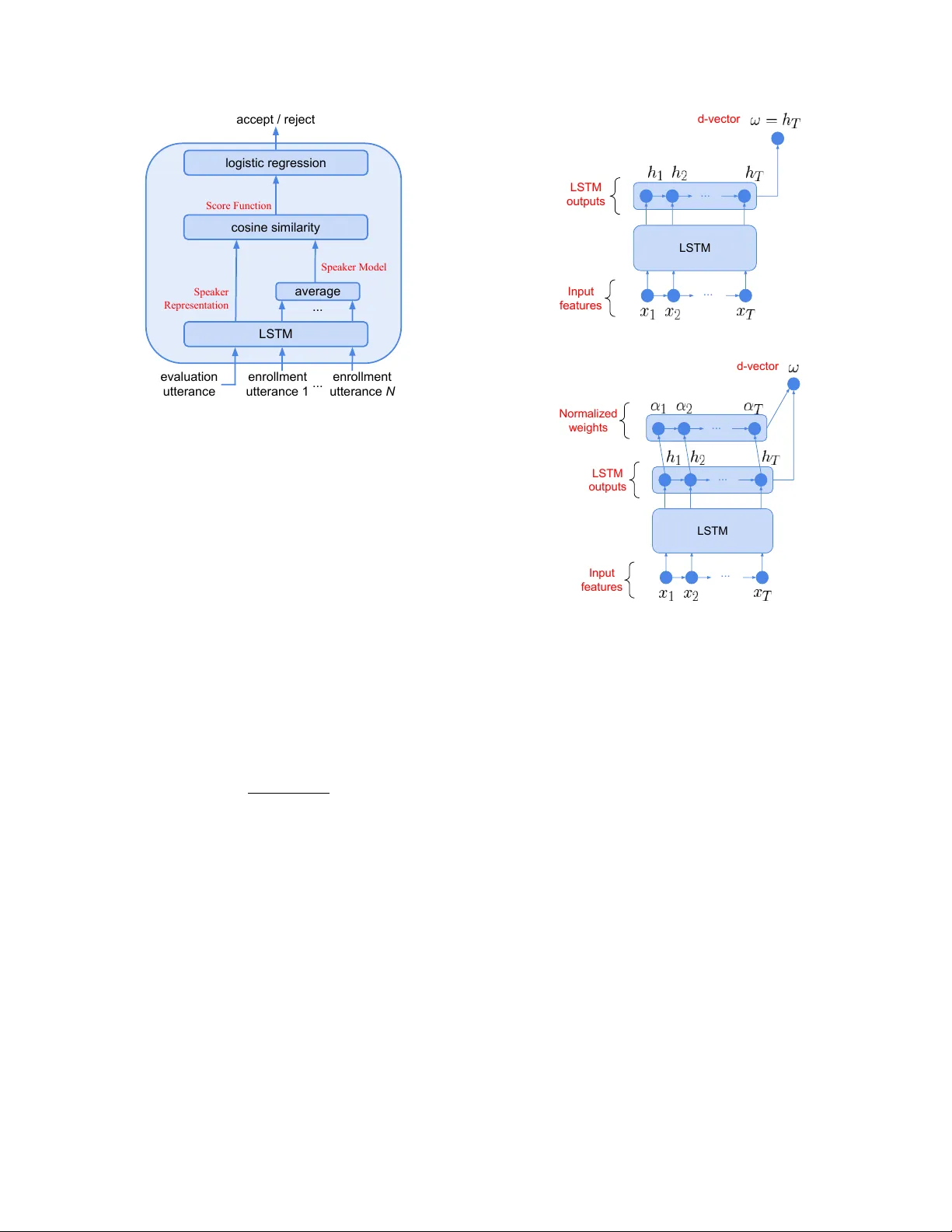
A TTENTION-B ASED MODELS FOR TEXT -DEPENDENT SPEAKER VERIFICA TION F A Rezaur Rahman Chowdhury ∗ W ashington State Univ ersity fchowdhu@eecs.wsu.edu Quan W ang, Ignacio Lopez Mor eno, Li W an Google Inc., USA { quanw , elnota , liwan } @google.com ABSTRA CT Attention-based models hav e recently shown great performance on a range of tasks, such as speech recognition, machine translation, and image captioning due to their ability to summarize relevant in- formation that expands through the entire length of an input se- quence. In this paper , we analyze the usage of attention mechanisms to the problem of sequence summarization in our end-to-end text- dependent speaker recognition system. W e explore dif ferent topolo- gies and their variants of the attention layer, and compare different pooling methods on the attention weights. Ultimately , we sho w that attention-based models can improv es the Equal Error Rate (EER) of our speaker verification system by relatively 14% compared to our non-attention LSTM baseline model. Index T erms — Attention-based model, sequence summariza- tion, speaker recognition, pooling, LSTM 1. INTR ODUCTION Speaker verification (SV) is the process of verifying, based on a set of reference enrollment utterances, whether an v erification utterance belongs to a known speaker . One subtask of SV is global password text-dependent speaker verification (TD-SV), which refers to the set of problems for which the transcripts of reference enrollment and verification utterances are constrained to a specific phrase. In this study , we focus on “OK Google” and “Hey Google” global pass- words, as they relate to the V oice Match feature of Google Home [ 1 , 2 ]. I-vector [ 3 ] based systems in combination with verification back-ends such as Probabilistic Linear Discriminant Analysis (PLD A) [ 4 ] have been the dominating paradigm of SV in previ- ous years. More recently , with the rising of deep learning [ 5 ] in various machine learning applications, more efforts have been fo- cusing on using neural networks for speaker verification. Currently , the most promising approaches are end-to-end integrated architec- tures that simulate the enrollment-v erification two-stage process during training. For example, in [ 6 ] the authors propose architectures that re- semble the components of an i-vector + PLDA system. Such archi- tecture allo wed to bootstrap the network parameters from pretrained i-vector and PLD A models for a better performance. Howe ver , such initialization stage also constrained the type of network architectures that could be used — only Deep Neural Networks (DNN) can be initialized from classical i-vector and PLD A models. In [ 7 ], we hav e shown that Long Short-T erm Memory (LSTM) networks [ 8 ] can achiev e better performance than DNNs for integrated end-to-end architectures in TD-SV scenarios. ∗ The author did this work during his intern at Google. Howe ver , one challenge in our architecture introduced in [ 7 ] is that, silence and background noise are not being well captured. Though our speaker v erification runs on a short 800ms window that is se gmented by the keyw ord detector [ 9 , 10 ], the phonemes are usu- ally surrounded by frames of silence and background noise. Ideally , the speaker embedding should be built only using the frames corre- sponding to phonemes. Thus, we propose to use an attention layer [ 11 , 12 , 13 ] as a soft mechanism to emphasize the most relev ant el- ements of the input sequence. This paper is organized as follows. In Sec. 2 , we first briefly revie w our LSTM-based d-v ector baseline approach trained with the end-to-end architecture [ 7 ]. In Sec. 3 , we introduce ho w we add the attention mechanism to our baseline architecture, cov ering differ - ent scoring functions, layer variants, and weights pooling methods. In Sec. 4 we setup experiments to compare attention-based mod- els against our baseline model, and present the EER results on our testing set. Conclusions are made in Sec. 5 . 2. B ASELINE ARCHITECTURE Our end-to-end training architecture [ 7 ] is described in Fig. 1 . For each training step, a tuple of one ev aluation utterance x j ∼ and N en- rollment utterances x kn (for n = 1 , · · · , N ) is fed into our LSTM network: { x j ∼ , ( x k 1 , · · · , x kN ) } , where x represents the features (log-mel-filterbank energies) from a fixed-length segment, j and k represent the speak ers of the utterances, and j may or may not equal k . The tuple includes a single utterance from speaker j , and N dif- ferent utterance from speaker k . W e call a tuple positi ve if x j ∼ and the N enrollment utterances are from the same speaker , i.e . , j = k , and negati ve otherwise. W e generate positiv e and negati ve tuples alternativ ely . For each utterance, let the output of the LSTM’ s last layer at frame t be a fixed dimensional vector h t , where 1 ≤ t ≤ T . W e take the last frame output as the d-vector ω = h T (Fig. 2a ), and build a new tuple: { ω j ∼ , ( ω k 1 , · · · , ω kN ) } . The centroid of tuple ( ω k 1 , · · · , ω kN ) represents the v oiceprint built from N utterances, and is defined as follows: c k = E n [ ω kn ] = 1 N N X n =1 ω kn k ω kn k 2 . (1) The similarity is defined using the cosine similarity function: s = w · cos( ω j ∼ , c k ) + b, (2) with learnable w and b . The tuple-based end-to-end loss is finally defined as: L T ( ω j ∼ , c k ) = δ ( j, k ) σ ( s ) +  1 − δ ( j, k )  1 − σ ( s )  . (3) evaluation utterance enrollment utterance 1 ... accept / reject Speaker Model Speaker Representation Score Function enrollment utterance N ... logistic regression cosine similarity average LSTM Fig. 1 : Our baseline end-to-end training architecture as introduced in [ 7 ]. Here σ ( x ) = 1 / (1 + e − x ) is the standard sigmoid function and δ ( j, k ) equals 1 if j = k , otherwise equals to 0 . The end-to-end loss function encourages a larger value of s when k = j , and a smaller value of s when k 6 = j . Consider the update for both positive and negati ve tuples — this loss function is very similar to the triplet loss in FaceNet [ 14 ]. 3. A TTENTION-B ASED MODEL 3.1. Basic attention layer In our baseline end-to-end training, we directly take the last frame output as d-vector ω = h T . Alternativ ely , we could learn a scalar score e t ∈ R for the LSTM output h t at each frame t : e t = f ( h t ) , t = 1 , · · · , T . (4) Then we can compute the normalized weights α t ∈ [0 , 1] using these scores: α t = exp( e t ) P T i =1 exp( e i ) , (5) such that P T t =1 α t = 1 . And finally , as sho wn in Fig. 2b , we form the d-vector ω as the weighted average of the LSTM outputs at all frames: ω = T X t =1 α t h t . (6) 3.2. Scoring functions By using dif ferent scoring functions f ( · ) in Eq. ( 4 ), we get different attention layers: • Bias-only attention, where b t is a scalar . Note this attention does not depend on the LSTM output h t . e t = f BO ( h t ) = b t . (7) • Linear attention, where w t is an m -dimensional vector , and b t is a scalar . e t = f L ( h t ) = w T t h t + b t . (8) ... Input features LSTM LSTM outputs d-vector ... (a) ... Input features ... LSTM LSTM outputs Normalized weights d-vector ... (b) Fig. 2 : (a) LSTM-based d-vector baseline [ 7 ]. (b) Basic attention layer . • Shared-parameter linear attention, where the m -dimensional vector w and scalar b are the same for all frames. e t = f SL ( h t ) = w T h t + b. (9) • Non-linear attention, where W t is an m 0 × m matrix, b t and v t are m 0 -dimensional vectors. The dimension m 0 can be tuned on a dev elopment dataset. e t = f NL ( h t ) = v T t tanh( W t h t + b t ) . (10) • Shared-parameter non-linear attention, where the same W , b and v are used for all frames. e t = f SNL ( h t ) = v T tanh( Wh t + b ) . (11) In all the abov e scoring functions, all the parameters are train- able within the end-to-end architecture [ 7 ]. 3.3. Attention layer variants Apart from the basic attention layer described in Sec. 3.1 , here we introduce two variants: cross-layer attention, and divided-layer at- tention. For cross-layer attention (Fig. 3a ), the scores e t and weights α t are not computed using the outputs of the last LSTM layer ... ... ... Last layer outputs d-vector 2nd-to-last layer outputs (a) ... ... ... ... d-vector Last layer outputs Part a Part b (b) Fig. 3 : T wo variants of the attention layer: (a) cross-layer attention; (b) divided-layer attention. { h t } 1 ≤ t ≤ T , but the outputs of an intermediate LSTM layer { h 0 t } 1 ≤ t ≤ T , e.g . the second-to-last layer: e t = f ( h 0 t ) . (12) Howe ver , the d-v ector ω is still the weighted a verage of the last layer output h t . For di vided-layer attention (Fig. 3b ), we double the dimension of the last layer LSTM output h t , and equally divide its dimension into two parts: part-a h a t , and part-b h b t . W e use part-a to build the d-vector , while using part-b to learn the scores: e t = f ( h b t ) , (13) ω = T X t =1 α t h a t . (14) 3.4. W eights pooling Another v ariation of the basic attention layer is that, instead of di- rectly using the normalized weights α t to average LSTM outputs, we can optionally perform maxpooling on the attention weights. This additional pooling mechanism can potentially make our net- work more robust to temporal variations of the input signals. W e hav e experimented with two maxpooling methods (Fig. 4 ): • Sliding windo w maxpooling: W e run a sliding window on the weights, and for each windo w , only keep the largest value, and set other values to 0. No pooling Sliding window maxpooling Global top- K maxpooling ( K =5) window 1 window 2 time Fig. 4 : Dif ferent pooling methods on attention weights. The t th pixel corresponds to the weight α t , and a brighter intensity means a lar ger value of the weight. • Global top- K maxpooling: Only keep the lar gest K values in the weights, and set all other values to 0. 4. EXPERIMENTS 4.1. Datasets and basic setup T o fairly compare different attention techniques, we use the same training and testing datasets for all our experiments. Our training dataset is a collection of anonymized user voice queries, which is a mixture of “OK Google” and “Hey Google”. It has around 150M utterances from around 630K speakers. Our test- ing dataset is a manual collection consisting of 665 speakers. It’s divided into two enrollment sets and two verification sets for each of “OK Google” and “Hey Google”. Each enrollment and evaluation dataset contains respectively , an average of 4.5 and 10 evaluation utterances per speaker . W e report the speaker verification Equal Error Rate (EER) on the four combinations of enrollment set and verification set. Our baseline model is a 3-layer LSTM, where each layer has dimension 128, with a projection layer [ 15 ] of dimension 64. On top of the LSTM is a linear layer of dimension 64. The acoustic parametrization consists of 40-dimensional log-mel-filterbank coef- ficients computed ov er a window of 25ms with 15ms of overlap. The same acoustic features are used for both keyw ord detection [ 10 ] and speaker verification. The keyword spotting system isolates segments of length T = 80 frames (800ms) that only contain the global password, and these segments form the tuples mentioned above. The two ke ywords are mixed together using the MultiReader technique introduced in [ 16 ]. 4.2. Basic attention layer First, we compare the baseline model with basic attention layer (Sec. 3.1 ) using dif ferent scoring function (Sec. 3.2 ). The results are shown in T able 1 . As we can see, while bias-only and linear attention bring little impro vement to the EER, non-linear attention 1 improv es the performance significantly , especially with shared parameters. 1 For the intermediate dimension of non-linear scoring functions, we use m 0 = 64 , such that W t and W are square matrices. T able 1 : Evaluation EER(%): Non-attention baseline model vs. basic attention layer using different scoring functions. T est data Non-attention Basic attention Enroll → V erify baseline f BO f L f SL f NL f SNL OK Google → OK Google 0.88 0.85 0.81 0.8 0.79 0.78 OK Google → Hey Google 2.77 2.97 2.74 2.75 2.69 2.66 Hey Google → OK Google 2.19 2.3 2.28 2.23 2.14 2.08 Hey Google → Hey Google 1.05 1.04 1.03 1.03 1.00 1.01 A verage 1.72 1.79 1.72 1.70 1.66 1.63 T able 2 : Evaluation EER(%): Basic attention layer vs. variants — all using f SNL as scoring function. T est data Basic f SNL Cross-layer Divided-layer OK → OK 0.78 0.81 0.75 OK → Hey 2.66 2.61 2.44 Hey → OK 2.08 2.03 2.07 Hey → Hey 1.01 0.97 0.99 A verage 1.63 1.61 1.56 T able 3 : Evaluation EER(%): Different pooling methods for atten- tion weights — all using f SNL and divided-layer . T est data No pooling Sliding window T op- K OK → OK 0.75 0.72 0.72 OK → Hey 2.44 2.37 2.63 Hey → OK 2.07 1.88 1.99 Hey → Hey 0.99 0.95 0.94 A verage 1.56 1.48 1.57 4.3. V ariants T o compare the basic attention layer with the two variants (Sec. 3.3 ), we use the same scoring function that performs the best in the pre- vious experiment: the shared-parameter non-linear scoring function f SNL . From the results in T able 2 , we can see that divided-layer at- tention performs slightly better than basic attention and cross-layer attention 2 , at the cost that the dimension of last LSTM layer is dou- bled. 4.4. W eights pooling T o compare different pooling methods on the attention weights as in- troduced in Sec. 3.4 , we use the di vided-layer attention with shared- parameter non-linear scoring function. For sliding window max- pooling, we experimented with dif ferent window sizes and steps, and found that a window size of 10 frames and a step of 5 frames perform the best in our ev aluations. Also, for global top- K max- pooling, we found that the performance is the best when K = 5 . The results are shown in T able 3 . W e can see that sliding window maxpooling further improv es the EER. W e also visualize the attention weights of a training batch for different pooling methods in Fig. 5 . An interesting observ ation is that, when there’ s no pooling, we can see a clear 4-strand or 3-strand pattern in the batch. This pattern corresponds to the “O-kay-Goo- gle” 4-phoneme or “Hey-Goo-gle” 3-phoneme structure of the key- words. 2 In our e xperiments, for cross-layer attention, scores are learned from the second-to-last layer . time utterance O kay Goo gle (a) No pooling (b) Sliding window maxpooling (c) Global top- K maxpooling Fig. 5 : V isualized attention weights for different pooling methods. In each image, x-axis is time, and y-axis is for different utterances in a training batch. (a) No pooling; (b) Sliding windo w maxpooling, where windo w size is 10, and step is 5; (c) Global top- K maxpool- ing, where K = 5 . When we apply sliding window maxpooling or global top- K maxpooling, the attention weights are much larger at the near-end of the utterance, which is easy to understand — the LSTM has accumu- lated more information at the near-end than at the be ginning, thus is more confident to produce the d-vector . 5. CONCLUSIONS In this paper, we experimented with dif ferent attention mechanisms for our keyw ord-based text-dependent speaker verification system [ 7 ]. From our experimental results, the best practice is to: (1) Use a shared-parameter non-linear scoring function; (2) Use a divided- layer attention connection to the last layer output of the LSTM; and (3) Apply a sliding window maxpooling on the attention weights. After combining all these best practices, we improv ed the EER of our baseline LSTM model from 1.72% to 1.48%, which is a 14% rel- ativ e improv ement. The same attention mechanisms, especially the ones using shared-parameter scoring functions, could potentially be used to improve text-independent speaker verification models [ 16 ] and speaker diarization systems [ 17 ]. 6. REFERENCES [1] Y ury Pinsky , “T omato, tomahto. google home now supports multiple users, ” https://www .blog.google/products/assistant/tomato-tomahto- google-home-now-supports-multiple-users, 2017. [2] Mihai Matei, “V oice match will al- low google home to recognize your v oice, ” https://www .androidheadlines.com/2017/10/voice-match- will-allow-google-home-to-recognize-your -voice.html, 2017. [3] Najim Dehak, Patrick J K enny , R ´ eda Dehak, Pierre Du- mouchel, and Pierre Ouellet, “Front-end factor analysis for speaker verification, ” IEEE T ransactions on Audio, Speech, and Language Processing , v ol. 19, no. 4, pp. 788–798, 2011. [4] Daniel Garcia-Romero and Carol Y Espy-W ilson, “ Analysis of i-vector length normalization in speaker recognition systems., ” in Interspeech , 2011, pp. 249–252. [5] Y ann LeCun, Y oshua Bengio, and Geoffrey Hinton, “Deep learning, ” Natur e , vol. 521, no. 7553, pp. 436–444, 2015. [6] Johan Rohdin, Anna Silnov a, Mireia Diez, Oldrich Plchot, Pa vel Matejka, and Lukas Burget, “End-to-end dnn based speaker recognition inspired by i-vector and plda, ” arXiv pr eprint arXiv:1710.02369 , 2017. [7] Georg Heigold, Ignacio Moreno, Samy Bengio, and Noam Shazeer , “End-to-end text-dependent speaker verification, ” in Acoustics, Speech and Signal Pr ocessing (ICASSP), 2016 IEEE International Confer ence on . IEEE, 2016, pp. 5115– 5119. [8] Sepp Hochreiter and J ¨ urgen Schmidhuber, “Long short-term memory , ” Neural computation , vol. 9, no. 8, pp. 1735–1780, 1997. [9] Guoguo Chen, Carolina Parada, and Georg Heigold, “Small- footprint keyword spotting using deep neural networks, ” in Acoustics, Speech and Signal Pr ocessing (ICASSP), 2014 IEEE International Confer ence on . IEEE, 2014, pp. 4087– 4091. [10] Rohit Prabhavalkar , Raziel Alvarez, Carolina Parada, Preetum Nakkiran, and T ara N Sainath, “ Automatic gain control and multi-style training for robust small-footprint keyw ord spotting with deep neural networks, ” in Acoustics, Speech and Signal Pr ocessing (ICASSP), 2015 IEEE International Confer ence on . IEEE, 2015, pp. 4704–4708. [11] Jan K Chorowski, Dzmitry Bahdanau, Dmitriy Serdyuk, Kyungh yun Cho, and Y oshua Bengio, “ Attention-based mod- els for speech recognition, ” in Advances in Neural Information Pr ocessing Systems , 2015, pp. 577–585. [12] Minh-Thang Luong, Hieu Pham, and Christopher D Manning, “Effecti ve approaches to attention-based neural machine trans- lation, ” arXiv pr eprint arXiv:1508.04025 , 2015. [13] Kelvin Xu, Jimmy Ba, Ryan Kiros, Kyunghyun Cho, Aaron Courville, Ruslan Salakhudinov , Rich Zemel, and Y oshua Ben- gio, “Sho w , attend and tell: Neural image caption generation with visual attention, ” in International Confer ence on Machine Learning , 2015, pp. 2048–2057. [14] Florian Schroff, Dmitry Kalenichenko, and James Philbin, “Facenet: A unified embedding for face recognition and clus- tering, ” in Pr oceedings of the IEEE Conference on Computer V ision and P attern Recognition , 2015, pp. 815–823. [15] Has ¸ im Sak, Andrew Senior , and Franc ¸ oise Beaufays, “Long short-term memory recurrent neural network architectures for large scale acoustic modeling, ” in F ifteenth Annual Conference of the International Speech Communication Association , 2014. [16] Li W an, Quan W ang, Alan Papir , and Ignacio Lopez Moreno, “Generalized end-to-end loss for speaker verification, ” arXiv pr eprint arXiv:1710.10467 , 2017. [17] Quan W ang, Carlton Downe y , Li W an, Philip Mansfield, and Ignacio Lopez Moreno, “Speaker diarization with lstm, ” arXiv pr eprint arXiv:1710.10468 , 2017.