Kalman-Takens filtering in the presence of dynamical noise

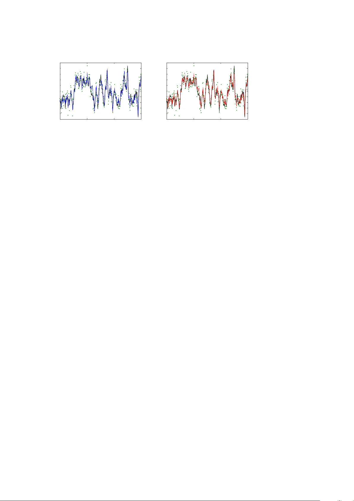
EPJ man uscript No. (will b e inserted b y the editor) Kalman-T ak ens filtering in the p resence of dynamical noise F ranz Hamilton 1 , T yrus Berry 2 , and Timoth y Sauer 2 , a 1 North Carolina State Universit y , Raleigh, NC 27695, USA 2 George Mason Univ ersity , F airfax, V A 22030, USA Abstract. The use of data assimilation for the merging of observ ed data with dynamical mo dels is b ecoming standard in mo dern physics. If a parametric mo del is kno wn, metho ds suc h as Kalman filtering ha ve b een developed for this purp ose. If no model is known, a hybrid Kalman-T akens metho d has b een recen tly introduced, in order to ex- ploit the adv an tages of optimal filtering in a nonparametric setting. This pro cedure replaces the parametric mo del with dynamics recon- structed from delay coordinates, while using the Kalman update for- m ulation to assimilate new observ ations. W e find that this hybrid ap- proac h results in comparable efficiency to parametric methods in iden- tifying underlying dynamics, even in the presence of dynamical noise. By combining the Kalman-T ak ens method with an adaptiv e filtering pro cedure w e are able to estimate the statistics of the observ ational and dynamical noise. This solv es a long standing problem of separating dy- namical and observ ational noise in time series data, which is esp ecially c hallenging when no dynamical mo del is sp ecified. 1 Intro duction Metho ds of data assimilation are hea vily used in geophysics and hav e become com- mon throughout ph ysics and other sciences. When a parametric, physically motiv ated mo del is a v ailable, noise filtering and forecasting in a v ariet y of applications are p os- sible. Although the original Kalman filter [1] applies to linear systems, more recent approac hes to filtering such as the Extended Kalman Filter (EKF) and Ensem ble Kalman Filter (EnKF) [2,3,4,5,6] allo w forecasting mo dels to use the nonlinear mo del equations to compute predictions that are close to optimal. In some cases, a mo del is not b e av ailable, and in other cases, all av ailable mo dels ma y b e inaccurate. In geoph ysical processes, basic principles may constrain a v ariable as a function of other driving v ariables in a known manner, but the driving v ariables ma y b e unmo deled or mo deled with large error [7,8,9,10]. Moreo ver, in numerical w eather prediction co des, physics on the large scale is typically sparsely mo deled [11,12]. Some recent work has considered the case where only a partial mo del is kno wn [13,14]. Under circumstances in whic h models are not av ailable, T akens’ method of attrac- tor reconstruction [15,16,17,18] has b een used to reconstruct physical attractors from a e-mail: tsauer@gmu.edu 2 Will b e inserted by the editor data. The dynamical attractor is t ypically represented b y v ectors of dela y coordinates constructed from time series observ ations, and approaches to prediction, control, and other time series applications ha v e been prop osed [19,20,21]. In particular, time series prediction algorithms lo cate the current p osition in the delay co ordinate represen ta- tion and use analogues from previously recorded data to establish a predictive sta- tistical model [22,23,24,25,26,27,28,29,30,31,32,33,34,35]. Ho w ever, T akens’ method is designed (and prov ed to work) for strictly deterministic systems, and the effects of noise, b oth dynamic and observ ational, is not thoroughly understo o d. Recen tly , a method was in tro duced that w ould merge T ak ens’ nonparametric at- tractor reconstruction approach with Kalman filtering. Since the mo del equations go verning the ev olution of the system are unknown, the dynamics are reconstructed nonparametrically using dela y-co ordinate vectors, and used to replace the mo del. The Kalman-T akens algorithm [36] is able to filter noisy data with comparable p er- formance to parametric filtering metho ds that hav e full access to the exact mo del. The fidelit y of this algorithm follows from the fact that T ak ens’ theorem [15] states roughly that in the large data limit, the equations can b e replaced by the data. The surprising fact, sho wn in [36], is that this fidelity is robust to observ ational noise which in v alidates the basic theory of [15], although a muc h more complex theory developed in [44] suggests such a robustness. In fact, by implemen ting the Kalman up date, it is suggested in [36] that the nonparametric representation of the dynamics is able to handle substan tial observ ational noise in the data. In this article we study the effects of dynamic noise (also kno wn as system noise or pro cess noise) on the Kalman-T ak ens algorithm. W e will verify the effectiv eness of the metho d on sto chastic differen tial equations with significant lev els of system noise, and sho w that nonparametric prediction can b e improv ed by the filter almost to the exten t of matc hing the p erformance of the exact parametric mo del. In section 2 w e presen t the sp ecifics of the Kalman-T akens metho d. A k ey to effective application of an y Kalman based algorithm is kno wing the cov ariance matrices of the system and observ ation noise, which are particularly difficult to separate when no mo del is kno wn. In section 3 we present an adaptive metho d for inferring statistics of the system and observ ational noise as part of the filtering procedure. The adaptive filtering method naturally complements the Kalman-T ak ens metho d by implicitly fitting a fully non- parametric sto chastic system to the data. These methods are combined in section 4, where applications to dynamical data with v ariable settings of delay co ordinates are explored. 2 Kalman-T ak ens filter W e recall the standard notion of the Kalman filter in the case where the mo del f and observ ation function g are kno wn. Consider a nonlinear stochastic system with n -dimensional state v ector x and m -dimensional observ ation vector y defined by x k +1 = f ( x k , t k ) + w k (1) y k = g ( x k , t k ) + v k where w k and v k are white noise pro cesses with cov ariance matrices Q and R , resp ec- tiv ely . W e b egin by describing the filtering pro cedure in the case when f and g are kno wn. W e are chiefly in terested in nonlinear systems, so w e will describ e a version of Kalman filtering that is common in this case. The ensemble Kalman filter (EnKF) [2] represen ts a nonlinear system at a given instan t as an ensemble of states. Here w e initialize the filter with state vector x + 0 = 0 n × 1 and cov ariance matrix P + 0 = Will b e inserted by the editor 3 I n × n . A t the k th step, the filter pro duces an estimate of the state x + k − 1 and the co v ariance matrix P + k − 1 , which estimates the cov ariance of the error b etw een the estimate x + k − 1 and the true state. In the unscented v ersion of EnKF [39], the singular v alue decomp osition is used to find the symmetric p ositive definite square ro ot S + k − 1 of the matrix P + k − 1 , allowing us to form an ensemble of E state vectors, where the i th ensem ble member is denoted x + i,k − 1 . The ensem ble v ectors x + i,k − 1 are formed b y adding and subtracting the columns of S + k − 1 to the estimate x + k − 1 to pro duce and ensem ble with mean x + k − 1 and cov ariance P + k − 1 [39,4,5]. In other words, the ensemble statistics matc h the current filter estimates of the mean and cov ariance. The ensem ble can also b e rescaled b y in troducing weigh ts for each ensemble member as described in [4,5]. The mo del f is applied to the ensemble, adv ancing it one time step, and then observ ed with function g . The mean of the resulting state ensemble giv es the prior state estimate x − k and the mean of the observed ensem ble is the predicted observ ation y − k . Denoting the cov ariance matrices P − k and P y k of the resulting state and observed ensem ble, and the cross-cov ariance matrix P xy k b et ween the state and observed en- sem bles, we define P − k = E X i =1  x − ik − x − k   x − ik − x − k  T + Q P y k = E X i =1  y − ik − y − k   y − ik − y − k  T + R P xy k = E X i =1  x − ik − x − k   y − ik − y − k  T . (2) Giv en the observ ation y k , the equations K k = P xy k ( P y k ) − 1 P + k = P − k − P xy k ( P y k ) − 1 P y x k x + k = x − k + K k  y k − y − k  . (3) up date the state and co v ariance estimates. W e will refer to this as the parametric filter, since a full set of model equations are assumed to be kno wn. The matrices Q and R are parameters which represent the co v ariance matrices of the system noise and the observ ation noise resp ectively . Often the true statistics of these noise processes are unkno wn, and examples in [40] hav e shown that accurate estimates of Q and R are crucial to obtaining a go o d estimate of the state. In section 3, w e describ e an algorithm developed in [40] for adaptive estimation of Q and R which w as developed for the case when the dynamical mo del f and observ ation function g are known. Con trary to (1), our assumption in this article is that neither the mo del f or observ ation function g are known, making outright implementation of the EnKF im- p ossible. Instead, the filter describ ed here requires no mo del while still leveraging the Kalman up date describ ed in (3). The idea is to replace the system ev olution, tradition- ally done through application of f , with adv ancemen t of dynamics nonparametrically using dela y-co ordinate v ectors. W e describe this metho d with the assumption that a single v ariable is observ able, sa y y , but the algorithm can b e easily generalized to m ultiple system observ ables. In addition, w e will assume in our examples that noise co v ariances Q and R are unknown and will b e up dated adaptively as in [40]. 4 Will b e inserted by the editor The idea b ehind T akens’ metho d is that given the observ able y k , the delay- co ordinate v ector x k = [ y k , y k − 1 , . . . , y k − d ] accurately captures the state of the dynamical system, where d is the num b er of dela ys. In the case where the noise v ariables are remov ed from (1), the vector x k pro v ably represen ts the state of the system for d + 1 > 2 n as sho wn in [15,17] (note that the embedding dimension is d + 1 since d delays are added to the original state). An extension of this result to the sto chastic system (1) can b e found in [44]. Current applications of T akens dela y-coordinate reconstruction hav e been restricted to fore- casting; typically by finding historical delay-coordinate states which are close to the curren t delay-coordinate state and interpolating these historical tra jectories. A sig- nifican t c hallenge in this metho d is finding ‘go o d’ neigh b ors, which accurately mirror the current state, esp ecially in real applications when b oth the current and historical states are corrupted b y observ ational noise. The goal of the Kalman-T akens filter is to quantify the uncertaint y in the state and reduce the noise using the Kalman filter. In order to in tegrate the T ak ens reconstruction into the Kalman filter, at eac h step of the filter an ensem ble of delay v ectors is formed. The adv ancemen t of this ensem ble forw ard in time requires a nonparametric technique to serv e as a lo cal proxy ˜ f for the unkno wn mo del f . Given a sp ecific delay co ordinate vector x k = [ y k , y k − 1 , . . . , y k − d ] , w e lo cate its N nearest neighbors (with resp ect to Euclidean distance) x i 1 , ..., x i N where x i j = [ y i j , y i j − 1 , . . . , y i j − d ] are found from the noisy training data. Once the neighbors are found, the known one step forecast v alues y i 1 +1 , y i 2 +1 , ..., y i N +1 are used with a lo cal mo del to predict y k +1 . In this article, we use a lo cally constant mo del which in its most basic form is an a verage of the nearest neighbors, namely ˜ f ( x k ) =  y i 1 +1 + y i 2 +1 + . . . + y i N +1 N , y k , . . . , y k − d +1  . This prediction can b e further refined by considering a weigh ted av erage of the nearest neighbors where the weigh ts are assigned as a function of the neighbor’s distance to the curren t dela y-coordinate v ector. Throughout the follo wing examples 20 neighbors were used. This process is rep eated to compute the one step forecast ˜ f applied to eac h member of the ensem ble. Once the full ensemble has been adv anced forw ard in time by ˜ f , the remaining EnKF algorithm is then applied using equations (2) as describ ed ab ov e, and our delay-coordinate state vector is up dated according to (3). This metho d w as called the Kalman-T akens filter in [36]. As an example we consider the following SDE based on the Lorenz-63 system [41] ˙ x = σ ( y − x ) + ξ ˙ W x ˙ y = x ( ρ − z ) − y + ξ ˙ W y (4) ˙ z = xy − β z + ξ ˙ W z where σ = 10, ρ = 28, β = 8 / 3 and ˙ W is white noise with unit v ariance. Assume we ha ve a noisy set of training data p oints y ( t k ) = x ( t k ) + η k where k = 1 , 2 , ..., M and y k = y ( t k ) is a direct observ ation of the x v ariable corrupted b y indep endent Gaussian p erturbations η k with mean zero and v ariance R o . Using this data, we w an t to dev elop a nonparametric forecasting metho d to predict future x Will b e inserted by the editor 5 0 5 10 15 Time -25 -20 -15 -10 -5 0 5 10 15 20 25 x (a) 0 5 10 15 Time -25 -20 -15 -10 -5 0 5 10 15 20 25 x (b) Fig. 1. Filtering comparison of the Lorenz-63 x v ariable when the system is affected by Gaussian dynamical noise with total v ariance of 2.4 (black solid line). Observ ations (green circles) of the sto c hastic signal p erturb ed by Gaussian observ ational noise with v ariance of 20 (signal RMSE of 4.49). (a) Parametric filter reconstruction (solid blue line) results in an RMSE of 2.34. (b) Kalman-T akens filter with 2 delays (solid red curve) results in RMSE of 2.95. v alues of the system. How ev er, due to the presence of the noise η k , outright application of a prediction metho d leads to inaccurate forecasts. If knowledge of (4) were a v ailable, the standard parametric filter could b e used to assimilate the noisy x observ ations to the mo del, generate a denoised estimate of the x v ariable, and simultaneously estimate the unobserved y and z v ariables. This denoised state estimate could then b e forecast forward in time using (4), and we refer to this pro cess and the parametric forecast. In contrast, the Kalman-T ak ens metho d assumes no knowledge of the underlying dynamics (4) or even the observ ation function. Instead, the Kalman-T akens metho d w orks directly with the noise observ ations y k and defines a proxy for the under- lying state b y the dela y vector [ y k , y k − 1 , . . . , y k − d ]. By applying the Kalman-T akens metho d to the entire training data set, we reduce the observ ation noise in the training data which will improv e future filtering and also provide b etter neighbors to improv e forecasting. Fig. 1 sho ws a comparison of ensemble Kalman filtering with and without the mo del. Fig. 1(a) shows the standard parametric EnKF applied to the x -co ordinate of the Lorenz SDE (4) with system noise v ariance ξ 2 = 0 . 8 (the total v ariance of the sys- tem noise is 2.4 since there are three indep endent noise v ariables), and observ ational noise v ariance R o = 20. Fig. 1(b) shows the Kalman-T akens filter applied to the same data. Compared to the SDE solution x ( t k ) without observ ational noise (black curve), the parametric filter fits slightly b etter, but the Kalman-T akens filter do es almost as w ell without knowing the mo del equations. A training set of M = 8000 points were used. Fig. 2 shows the same comparison with a higher lev el of system noise ξ 2 = 5 (total system noise v ariance is 15). 3 A daptive estimation of Q and R A persistent problem in time series analysis is distinguishing system noise from obser- v ational noise. This is a particularly important issue since observ ational noise distorts the forecast, and needs to b e remo ved, whereas the system noise affects the future of the system and th us should not b e remov ed. In other w ords, the state estimate that 6 Will b e inserted by the editor 0 5 10 15 Time -25 -20 -15 -10 -5 0 5 10 15 20 25 x (a) 0 5 10 15 Time -25 -20 -15 -10 -5 0 5 10 15 20 25 x (b) Fig. 2. Filtering comparison of the Lorenz-63 x v ariable when the system is affected by Gaussian dynamical noise with total v ariance of 15 (black solid line). Observ ations (green circles) of the sto c hastic signal p erturb ed by Gaussian observ ational noise with v ariance of 20 (signal RMSE of 4.49). (a) Parametric filter reconstruction (solid blue line) results in an RMSE of 3.21. (b) Kalman-T akens filter with 2 delays (solid red curve) results in RMSE of 3.29. will give the optimal forecast includes the system noise p erturbation, but do es not include any of the observ ation noise p erturbations. While obtaining this p erfect esti- mate is t ypically impossible, getting as close as possible requires kno wing the statistics and correlations of the tw o noise pro cesses. This is captured in the structure of the Kalman equations (2) and (3) which gives the prov ably optimal estimate of the state for linear systems with additiv e Gaussian system and observ ation noise. The presence of the noise cov ariance matrices Q and R in the Kalman equations sho ws how these parameters determine the optimal estimate. Since w e cannot assume that the noise cov ariance matrices Q and R are known, w e used a rece n tly-dev elop ed metho d [40] for the adaptive fitting of these matrices as part of the filtering algorithm. The key difficult y in estimating these cov ariances is disam biguating the tw o noise sources. The metho d of [40] is based on the fact that system noise p erturbations affect the state at future times, whereas observ ation noise p erturbations only affect the curren t time. The method uses the inno v ations  k ≡ y k − y − k in observ ation space from (2) to up date the estimates Q k and R k of the co v ariances Q and R , resp ectively , at step k of the filter. In order to estimate these tw o quan tities, we will compute tw o statistics of the innov ations. The first statistic is the outer pro duct  k  > k and the second statistic is the lagged outer product  k  > k − 1 . Intuitiv ely , the first statistic only includes infor- mation ab out the observ ation noise cov ariance, whereas the second statistic contains information ab out the system noise co v ariance. W e produce empirical estimates Q e k − 1 and R e k − 1 of Q and R based on the inno- v ations at time k and k − 1 using the form ulas P e k − 1 = F − 1 k − 1 H − 1 k  k  T k − 1 H − T k − 1 + K k − 1  k − 1  T k − 1 H − T k − 1 Q e k − 1 = P e k − 1 − F k − 2 P a k − 2 F T k − 2 R e k − 1 =  k − 1  T k − 1 − H k − 1 P f k − 1 H T k − 1 . (5) It w as shown in [40] that P e k − 1 is an empirical estimate of the background cov ariance at time index k − 1. Notice that (5) requires lo cal linearizations F k − 1 of the dynamics and H k − 1 of the observ ation function. While there are man y metho ds of finding these Will b e inserted by the editor 7 0 5 10 15 System Noise Variance 0 2 4 6 8 10 12 14 16 18 20 trace(Q est ) (a) 0 5 10 15 System Noise (variance) 0 2 4 6 8 10 12 14 16 18 20 22 R est (b) Fig. 3. Adaptive estimation of the filter Q and R matrices. Parametric filter (solid blue curv e), Kalman-T akens with 2 dela ys (solid red curv e), Kalman-T akens with 4 delays (dotted red curv e) (a) System noise estimate Q est (b) Observ ation noise estimate R est linearizations, we use the metho d introduced in [40] and used in [36] whic h is based on a linear regression. In particular, to determine F k − 1 a linear regression is applied b et ween the ensemble b efore and after the dynamics ˜ f are applied. Similarly , to determine H k − 1 a linear regression is applied b etw een the ensemble b efore and after the observ ation function is applied. Notice that this pro cedure requires us to sav e the linearizations F k − 2 , F k − 1 , H k − 1 , H k , innov ations  k − 1 ,  k , and the analysis P a k − 2 and Kalman gain matrix, K k − 1 , from the k − 1 and k − 2 steps of the EnKF. T o find stable estimates of Q and R we combine the noisy estimates Q e k − 1 and R e k − 1 (whic h are also low-rank b y construction) using an exp onential moving av erage Q k = Q k − 1 + ( Q e k − 1 − Q k − 1 ) /τ R k = R k − 1 + ( R e k − 1 − R k − 1 ) /τ . (6) where τ is the windo w of the mo ving a v erage. F or further details on the estimation of Q and R we refer the reader to [40,36]. In Fig. 3 we show the final estimates trace( Q est ) and R est from applying the adaptiv e filter to the sto chastic Lorenz system (4) with v arious system noise levels 3 ξ 2 (note that the factor 3 giv es the total v ariance of the three stochastic forcing v ariables which is compared to trace( Q est ) whic h is also a total v ariance). In Fig. 3(b) w e show that all of the filter metho ds obtain reasonably accurate estimates of the true observ ation noise R o = 20, and the results are v ery robust to the amount of system noise. In Fig. 3(a) we first note that the parametric filter with the p erfect mo del obtains a go o d estimate (blue, solid curve) of the true system noise (black, dashed curve). Secondly , we note that the trace of Q est for the Kalman-T akens filters b oth increase with increasing system noise, without distorting the estimate of the observ ation noise (as shown in Fig. 3(b)). Notice that the T akens reconstruction corresp onds to a highly nonlinear transformation of the state space, and that even the dimension of the state space changes. Since this nonlinear transformation ma y stretc h or contract the state space in a complicated wa y , it is not particularly surprising that the v ariance of the sto chastic forcing in the delay-em bedding space has a differen t magnitude than the original system noise v ariance. The exact relationship b et ween these tw o sto chastic forcings is highly nontrivial, and the spatially homogeneous and uncorrelated system noise of (4) may easily b ecome inhomogeneous and correlated in the reconstructed dynamics. 8 Will b e inserted by the editor 0 5 10 15 System Noise (variance) 0 0.5 1 1.5 2 2.5 RMSE (a) 0 5 10 15 System Noise (variance) 0 1 2 3 4 5 RMSE (b) 0 5 10 15 System Noise (variance) 0 1 2 3 4 5 6 7 8 RMSE (c) Fig. 4. Reconstructing the noisy Lorenz-63 x v ariable under increasing levels of dynamical noise. Observ ations of sto chastic signal p erturb ed by Gaussian observ ational noise with v ariance (a) 5, (b) 20 and (c) 60 resulting in signal error level (dotted blac k line). P arametric filter (solid blue line), Kalman-T akens filter with 2 delays (solid red line) and Kalman- T akens filter with 4 delays (dotted red line) reconstruction accuracy shown. Error bars denote standard error ov er 5 realizations. As the amount of dynamical noise increases, the Kalman-T akens filter has p erformance very similar to the parametric filter, which has access to the full mo del. 4 F iltering dynamical noise The Kalman-T akens filter was introduced in [36], which considered deterministic dy- namical systems with only observ ation noise. In section 2, w e show ed that the filter is also robust to dynamical noise, and in this section we quantify this fact for sto chastic systems suc h as (4) that include b oth system and observ ation noise. In Fig. 4 we compare the Kalman-T ak ens filters (red curves) to the parametric filter (blue curve) as a function of the system noise v ariance 3 ξ 2 for v arious levels of observ ation noise. In Fig. 4 the observ ation noise, which is the error betw een the observed signal and the true state, is denoted b y the black dotted line in each subfigure. Each filter ob- tains a dramatic denoising of the observ ations relative to the observ ation noise levels R o = 5 , 20 , and 60 in Figs. 4(a,b,c) resp ectively . In each case, for large observ ation noise the Kalman-T akens filter p erformance is comparable to the parametric filter, and only at very low system noise do es the parametric filter hav e a slight adv an tage. This illustrates the robustness that the Kalman-T akens filter has to mo del error since it makes no assumption on the form of the mo del, unlike the parametric filter which p ossesses the p erfect mo del. W e also explored the robustness of the Kalman-T akens filter to the num ber of dela ys d used in the T akens dela y-em b edding. F or d = 2 the e m b edding dimension is d + 1 = 3, which is the minim um dimension needed to embed the attractor of the deterministic Lorenz-63 system. How ev er, the theoretical guarantee of the T akens em b edding theory requires d + 1 > 2 n where n is the attractor dimension, which requires an embedding dimension of d + 1 = 5 (the attractor of the deterministic Lorenz-63 system is slightly larger than 2). As shown in Fig. 4(a,b) the d = 2 (red, solid curve) and d = 4 (red, dotted curve) hav e similar performance except at v ery low system noise levels, where d = 4 has a slight adv an tage. Notice that when very little noise is present, the longer that tw o tra jectories agree, the closer the corresp onding states are, so for small noise, w e exp ect long delays to help find b etter neighbors. Ho wev er, in the presence of system noise, this breaks do wn. Two tra jectories may b e very close in the past but recent sto c hastic forcing may cause them to quickly div erge. Moreo v er, as noise is added, it b ecomes increasingly difficult to distinguish states, and adding delays is merely adding more dimensions whic h could coinciden tally Will b e inserted by the editor 9 0 0.2 0.4 0.6 0.8 1 Forecast Horizon 0 1 2 3 4 5 6 7 8 9 10 11 RMSE (a) 0 0.2 0.4 0.6 0.8 1 Forecast Horizon 0 1 2 3 4 5 6 7 8 9 10 11 RMSE (b) Fig. 5. F orecast accuracy when predicting Lorenz-63 from 8000 noisy training data. (a) System influenced by Gaussian dynamical noise with v ariance of 0.8. (b) System influenced b y Gaussian dynamical noise wtih v ariance of 5. Observ ations perturb ed b y Gaussian ob- serv ational noise with v ariance of 20. Prediction results shown when the training data are not filtered (solid black curv e), filtered by the parametric filter (solid blue curve), Kalman- T akens filter with 2 dela ys (solid red curve) and Kalman-T akens filter with 4 delays (dotted red curv e) is used. Results av eraged ov er 1000 realizations. agree without implying the states are similar. This is shown in Fig. 4(c) where d = 2 outp erforms d = 4 in the presence of large observ ation noise. Similarly , in all of Fig. 4 w e note that as the system noise increases, the v alue of knowing the true model (4) b ecomes negligible as the d = 2 Kalman-T akens p erformance is indistinguishable from the parametric filter. Finally , we sho w in Fig. 5 that the Kalman-T akens filter achiev es forecast p erfor- mance comparable to the p erfect mo del. The Kalman-T akens impro ves forecasting in tw o wa ys. First, by running the Kalman-T akens filter on the historical training data, we significantly reduce the observ ation noise, whic h allo ws for b etter analog forecasting. Second, the Kalman-T akens filter gives a go o d estimate of the current state, whic h leads to an impro v ed forecast. Ultimately , T akens based forecasting re- lies on finding go o d neighbors in delay-em b edding space since these neighbors are in terp olated to form the forecast. Finding goo d neighbors requires both a goo d esti- mate of the current state, and historical data with small observ ation noise; and the Kalman-T ak ens filter improv es b oth of these. As a baseline, we used the unfiltered delay-em bedding and found neighbors in the ra w delay-em bedded historical data, and the RMSE of this forecast metho d is shown in Fig. 5 (black solid curve) as a function of the forecast horizon. The time zero forecast is simply the initial estimate, and for the blac k solid curve the RMSE at time zero corresp onds to the observ ation noise lev el (since the initial state is simply the unfiltered current observ ation). The low er RMSE of the filtered estimates (red and blue curv es) at time zero in Fig. 5 shows ho w the filter impro v es the initial estimate of the state. Similarly , the long term forecast con v erges to the av erage of the historical training data (since w e use an ensem ble forecast which are uncorrelated in the long term). The low er RMSE of the filtered forecasts (red curv es) compared to the raw data (blac k curve) in Fig. 5 sho ws that denoising the historical data giv es an impro v ed estimate of the long term statistics of the SDE. Moreov er, since the red curv es are v ery close to the blue curve in Fig. 5 we conclude that the Kalman-T akens is able to impro ve the historical data and estimate the curren t state with sufficient accuracy to matc h the parametric filter and forecast using the p erfect mo del. 10 Will b e inserted by the editor 5 Summa ry T raditional data assimilation is predicated on the existence of an accurate mo del for the dynamics. In this article, we hav e sho wn that the Kalman-T akens filter provides an alternative when no mo del is av ailable. Although it might be exp ected that dy- namical noise w ould b e an obstruction to the delay-coordinate embedding that is necessary to reconstruct the attractor, we find b y numerical experiment that filter- ing and forecasting applications are not hamp ered significantly more than for the parametric filter. This rep ort is a feasibility study , and leav es op en several interesting questions ab out how to optimally apply the algorithm. In particular, the role of the num ber of dela ys, neighborho o d size, as well as their relation to the EnKF parameters are still not w ell understo o d, and are deserving of further inv estigation. References 1. R. Kalman, J. Basic Eng. 82 (1960) 35. 2. E. Kalna y , Atmospheric mo deling, data assimilation, and predictability (Cam bridge Univ. Press, 2003). 3. G. Evensen, Data assimilation: The Ensemble Kalman Filter (Springer: Heidelberg, 2009). 4. S. Julier, J. Uhlmann, and H. Durrant-Wh yte, IEEE T rans. Automat. Control 45 (2000) 477. 5. S. Julier, J. Uhlmann, and H. Durrant-Wh yte, Pro c. IEEE 92 (2004) 401. 6. S. Sch iff, Neural control engineering (MIT Press, 2012). 7. R. H. Reichle and R. D. Koster, Geophysical Research Letters 32 (2005). 8. H. Hersbac h, A. Stoffelen, and S. De Haan, Journal of Geoph ysical Research: Oceans (1978–2012) 112 (2007). 9. H. Arnold, I. Moroz, and T. Palmer, Philosophical T ransactions of the Roy al So ciety A: Mathematical, Ph ysical and Engineering Sciences 371 (2013) 20110479. 10. T. Berry and J. Harlim, Pro ceedings of the Roy al Society A: Mathematical, Physical and Engineering Science 470 (2014) 20140168 . 11. E. N. Lorenz and K. A. Emanuel, J. Atmos. Sci. 55 (1998) 399. 12. T. N. Palmer, Quart. J. Roy . Met. So c. 127 (2001) 279. 13. F. Hamilton, T. Berry , and T. Sauer, Physical Review E 92 (2015) 010902 . 14. T. Berry and J. Harlim, Journal of Computational Physics 308 (2016) 305. 15. F. T akens, Lecture Notes in Math. Springer-V erlag: Berlin 898 (1981). 16. N. P ack ard, J. Crutchfield, D. F armer, and R. Shaw, Phys. Rev. Lett. 45 (1980) 712. 17. T. Sauer, J. Y orke, and M. Casdagli, J. Stat. Phys. 65 (1991) 579. 18. T. Sauer, Phys. Rev. Lett. 93 (2004) 198701. 19. E. Ott, T. Sauer, and J. A. Y ork e, Coping with chaos: Analysis of chaotic data and the exploitation of cha otic systems (Wiley New Y ork, 1994). 20. H. Abarbanel, Analysis of observed chaotic data (Springer-V erlag, New Y ork, 1996). 21. H. Kantz and T. Schreiber, Nonlinear time series analysis (Cambridge Universit y Press, 2004). 22. J. F armer and J. Sidorowic h, Phys. Rev. Lett. 59 (1987) 845. 23. M. Casdagli, Physica D: Nonlinear Phenomena 35 (1989) 335. 24. G. Sugihara and R. M. May , Nature 344 (1990) 734. 25. L. A. Smith, Physica D: Nonlinear Phenomena 58 (1992) 50. 26. J. Jimenez, J. Moreno, and G. Ruggeri, Phys. Rev. A 45 (1992) 3553. 27. T. Sauer, in Time Series Prediction: F orecasting the F uture and Understanding the Past (Addison W esley , 1994), 175–193. 28. G. Sugihara, Philosophical T ransactions of the Roy al So ciet y of London. Series A: Phys- ical and Engineering Sciences 348 (1994) 477. 29. C. G. Schroer, T. Sauer, E. Ott, and J. A. Y orke, Phys. Rev. Lett. 80 (1998) 1410. Will b e inserted by the editor 11 30. D. Kugium tzis, O. Ling jaerde, and N. Christophersen, Physica D: Nonlinear Phenomena 112 (1998) 344. 31. G. Y uan, M. Lozier, L. Pratt, C. Jones, and K. Helfric h, J. Geoph ys. Res. 109 (2004) C08002 . 32. C.-H. Hsieh, S. M. Glaser, A. J. Lucas, and G. Sugihara, Nature 435 (2005) 336. 33. C. C. Strelioff and A. W. Hubler, Phys. Rev. Lett. 96 (2006) 044101. 34. S. Regonda, B. Ra jagopalan, U. Lall, M. Clark, and Y.-I. Mo on, Nonlin. Pro c. in Geo- ph ys. 12 (2005) 397. 35. B. Schelter, M. Winterhalder, and J. Timmer, Handb ook of time series analysis: recent theoretical dev elopments and applications (John Wiley and Sons, 2006). 36. F. Hamilton, T. Berry , and T. Sauer, Phys. Rev. X 6 (2016) 011021. 37. T. Berry , D. Giannakis, and J. Harlim, Phys. Rev. E 91 (2015) 032915. 38. T. Berry and J. Harlim, Physica D 320 (2016) 57. 39. D. Simon, Optimal State Estimation: Kalman, H ∞ , and Nonlinear Approac hes (John Wiley and Sons, 2006). 40. T. Berry and T. Sauer, T ellus A 65 (2013) 20331. 41. E. Lorenz, J. Atmos. Sci. 20 (1963) 130. 42. E. N. Lorenz, in Pro ceedings: Seminar on predictabilit y (AMS, Reading, UK, 1996), 1-18. 43. A. Sitz, U. Sch w arz, J. Kurths, and H. V oss, Physical Review E 66 (2002) 16210. 44. J. Stark, D.S. Bro omhead, M.E. Davies, J. Huke, Journal of Nonlinear Science 13 (2003) 519.