Generating Random Networks Without Short Cycles

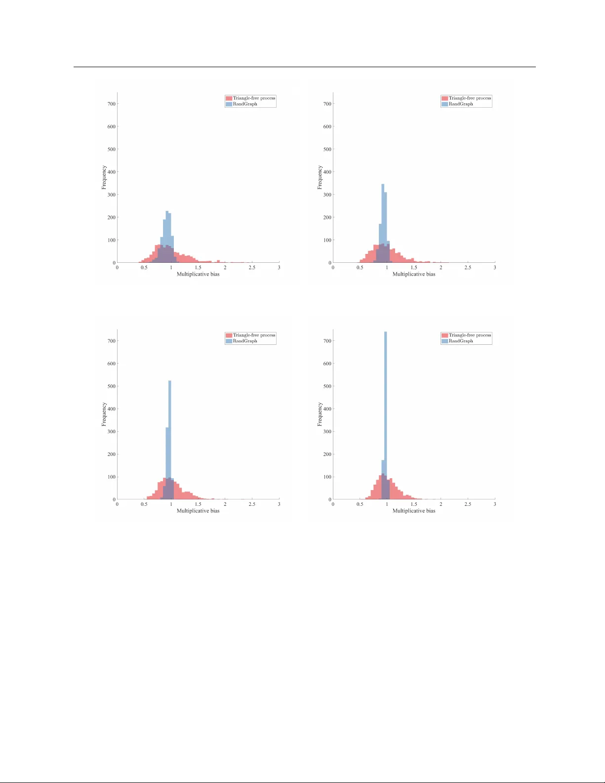
Generating Random Net w orks Without Short Cycles Mohsen Ba yati Graduate School of Business, Stanford Universit y , Stanford, CA 94305, ba yati@stanford.edu Andrea Mon tanari Departments of Electrical Engineering and Statistics, Stanford, CA 94305, mon tanar@stanford.edu Amin Sab eri Departments of Managemen t Science and Engineering and Institute for Computational and Mathematical Engineering, Stanford, CA 94305, saberi@stanford.edu Random graph generation is an imp ortant tool for studying large complex netw orks. Despite abundance of random graph mo dels, constructing models with application-driven constrain ts is po orly understo o d. In order to adv ance state-of-the-art in this area, we focus on random graphs without short cycles as a st ylized family of graphs, and prop ose the RandGraph algorithm for randomly generating them. F or any constan t k , when m = O ( n 1+1 / [2 k ( k +3)] ), RandGraph generates an asymptotically uniform random graph with n vertices, m edges, and no cycle of length at most k using O ( n 2 m ) op erations. W e also characterize the approximation error for ﬁnite v alues of n . T o the best of our kno wledge, this is the ﬁrst p olynomial-time algorithm for the problem. RandGraph w orks by sequentially adding m edges to an empty graph with n vertices. Recently , suc h sequen tial algorithms ha ve been successful for random sampling problems. Our main contributions to this line of research includes introducing a new approach for sequentially approximating edge-sp eciﬁc probabilities at eac h step of the algorithm, and pro viding a new method for analyzing suc h algorithms. Key wor ds : Net work mo dels, Poisson approximation, Random graphs 1. Intro duction Recen tly , a common ob jectiv e in man y application areas has been extracting information from data sets that con tain a netw ork structure. Examples of such data are the Internet, social netw orks, biological net works, or healthcare net works suc h as netw ork of physician referrals. In the last example, consider the question “ho w is the netw ork of ph ysician referrals formed?”. Answering this question could allow p olicy makers to inﬂuence the formation of the net w ork with the ob jective of impro ving qualit y of care. This could be ac hiev ed b y rew arding referrals to higher qualit y ph ysicians and p enalizing referrals to low er p erforming physicians. Unfortunately , empirical analysis of such net work related questions is challenging since in most cases researchers hav e access to a single net work or a few snapshots of it o ver time. Sp eciﬁcally , the small n umber of samples renders the estimation part of an y parametric net work formation mo del unreliable ( Chandrasekhar 2015 ). A p opular approach in statistical data analysis, when facing small num b er of observ ations, is b o otstrap ( Efron 1979 ) whic h increases the n umber of observ ations by creating random re-samples 1 2 of the original data. How ever, creating random copies of netw orks can b e computationally exp en- siv e. F or example, if the aim is to create a random cop y of the physician referral net w ork while k eeping the n um b er of neigh b ors (degree) of eac h node ﬁxed, the problem b ecomes NP hard in general ( W ormald 1999 ). The prop ert y of ﬁxing the num b er of neighbors is relev an t when it is desired to control for v ariations in abilities of the physicians to form working relationships. Simi- larly , one could b e interested in creating random copies of a netw ork when certain sub-structures should b e preserv ed or av oided. This problem in general is unsolved from a theoretical p oin t of view except for few examples where eﬃcien t algorithms are prop osed ( W ormald 1999 ). Therefore, practitioners use non-rigorous heuristic mo dels of random net works whic h may lead to incorrect (biased) estimates, see ( Milo et al. 2002 ) for suc h a heuristic. The ob jectiv e of this pap er is to adv ance state-of-the-art in this line of research by prop osing a new algorithm and analysis tec hnique. W e presen t the approach for a st ylized sub class of problems, generating random graphs without short cycles, and leav e extensions to other substructures for future research. While our emphasis in this pap er is on adv ancing the metho dology , and the family of graphs without short cycles is selected as an example of open problems in this area, we note that randomly generating graphs from this family has practical implications in information theory . Suc h graphs are used in designing lo w density parity c heck (LDPC) co des that can achiev e Shannon capacit y for transmitting messages in a noisy en vironment ( Ric hardson and Urbanke 2008 ). 1.1. Contributions W e presen t a simple and eﬃcien t algorithm, RandGraph , for randomly generating simple graphs without short cycles. F or an y constan t k , α ≤ 1 / [2 k ( k + 3)], and m = O ( n 1+ α ), RandGraph generates an asymptotically uniform random graph with n vertices, m edges, and no cycle of length k or smaller. RandGraph uses O ( n 2 m ) op erations in exp ectation. In addition, for ﬁnite v alues of n , we calculate the appro ximation error. T o the b est of our knowledge, this is the ﬁrst p olynomial-time algorithm for the problem. RandGraph starts with an empty graph and sequentially adds m edges b et ween pairs of non- adjacen t v ertices. In every step, tw o distinct v ertices i , j with distance at least k are selected with probabilit y p ij , and the edge ( ij ) is added to the graph. The most crucial step, computing p ij , is obtained by ﬁnding a sharp estimate for the n umber of extensions of the partially constructed graph, G t , that con tain ( ij ) and ha ve no cycle of length at most k . This estimation is done b y computing the exp ected n um b er of small cycles pro duced if the rest of the edges are added uniformly at random, using a P oisson appro ximation. Our analysis of RandGraph inv oles three approximation steps. First w e appro ximate random graphs that hav e m edges and n vertices with Erd¨ os-R ´ en yi (ER) graphs where eac h edge app ears 3 indep enden tly with probabilit y m/  n 2  . The second appro ximation uses Janson inequality ( Janson 1990 ) for estimating the probabilit y 1 that random ER graphs ha v e no cycle of length at most k . These t w o appro ximations pro vide us with an estimate for the uniform distribution on the family of graphs without cycles of length at most k . In the ﬁnal and third step, w e appro ximate G t with ER graphs with edge density t/m to estimate the output distribution of RandGraph , and to sho w that it is asymptotically equal to the uniform distribution. W e emphasize that these appro ximations are easy when m = O ( n ), and our main con tribution is to show that they are sharp even when the n umber of edges is sup er-linear in n , namely when m = O ( n 1+ α ) for small v alues of α . W e also provide a theoretical and empirical comparison betw een RandGraph and the well-kno wn triangle-fr e e pro cess that has recently b een sho wn to produce triangle-free graphs (our problem when k = 3) with an almost uniform distribution ( P ontiv eros et al. 2013 , Bohman and Keev ash 2013 ). The comparison shows that the output distribution of RandGraph is m uch closer to the uniform distribution. 1.2. Organization of the P ap er The rest of the pap er is organized as follo ws. § 2 discusses related research. Description of RandGraph and the main result are presen ted in § 3 . § 4 pro vides the main idea b ehind RandGraph follow ed by its analysis in § 5 . An eﬃcien t implementation of RandGraph is presented in § 6 and a comparison with the triangle-free pro cess is given in § 7 . Finallly , an extension of RandGraph to bipartite graphs with giv en degrees is discussed in § 8 . 2. Related Literature Random graph mo dels hav e been used in a wide v ariety of researc h areas. F or example they are used in determining the eﬀect of ha ving o verw eight friends in adolescen t ob esity ( V alen te et al. 2009 ), in studying social netw orks that result from unco ordinated random connections created b y individuals ( Jac kson and W atts 2002 ), in mo deling emergence of the world wide w eb as an endogenous phenomena ( P apadimitriou 2001 ) with certain top ological prop erties ( Kleinberg 2000 , Newman 2003 ), and in sim ulating netw orking proto cols on the In ternet top ology ( T angmunarunkit et al. 2002 , F aloutsos et al. 1999 , Medina et al. 2000 , Bu and T owsley 2002 ). In information theory , random graphs are used to construct LDPC co des that can approac h Shannon capacity ( Richardson and Urbanke 2008 ), sp eciﬁcally , when the graphs represen ting the co des are selected uniformly at random from the se t of bipartite graphs with giv en degree sequences 1 W e note that using the Poisson approximation method in § 6.2 of ( Janson et al. 2000 ) one can estimate this probabilit y with an additiv e error that conv erges to 0 with a rate that is inv ersely polynomial in n . Ho wev er, here w e require a stronger approximation since w e need a multiplicativ e error that conv erges to 1. This would require the additive error to con verge to zero faster than the probabilit y of the ev ent itself whic h is exp onentially small in n when m = O ( n 1+ α ). 4 ( Amraoui et al. 2007 , Ch ung et al. 2001 , Lub y et al. 1997 ). While these random graphs guarantee optimal p erformances asymptotically , in practice the LDPC graph has b et ween 10 3 and 10 5 no des where it is sho wn that the existence of a small n umber of subgraphs spoil the co de performances ( Di et al. 2002 , Ric hardson 2003 , Ko etter and V on tob el 2003 ). The present pap er studies a sp eciﬁc class of suc h subgraphs (short cycles), but we exp ect our approach to b e applicable to other subgraphs as w ell. In addition, for the sake of simplicity , we present the relev an t pro ofs only for the problem of generating random graphs without short cycles (not necessarily bipartite nor with prescrib ed degrees). Then we will adapt the algorithm for generating random bipartite graphs with given degree sequences that ha ve no short cycles 2 . Generalizing pro ofs to this case is cum b ersome but w e exp ect that to b e conceptually straigh tforward. Random graph generation has also b een studied extensively as an important theoretical problem ( W ormald 1999 , Ioannides 2006 ). F rom a theoretical p ersp ectiv e, our w ork is related to the following problem. Consider a graph prop ert y P that is preserv ed b y remov al of any edge from the graph. It is a standard problem in extremal graph theory to determine the largest m such that there exists a graph with n v ertices and m edges ha ving prop erty P . Low er b ounds on m can b e obtained through the analysis of greedy algorithms. Such algorithms proceed b y sequen tially choosing an edge uniformly from edges whose inclusion would not destroy property P , adding that to the graph, and rep eating the pro cedure until no further edge can b e added. The resulting graph is a random maximal P -graph. The question of ﬁnding the num b er of edges of a random maximal P - graph for several properties P has attracted considerable attention ( Rucinski and W ormald 1992 , Erd˝ os et al. 1995 , Sp encer 1995 , Bollob´ as and Riordan 2000 , Osthus and T araz 2001 , Bohman and Keev ash 2010 , W olfovitz 2011 , Pon tiveros et al. 2013 , Bohman and Keev ash 2013 , W arnke 2014 ). In particular, when P is the prop ert y that the graph has no cycles of length k , the ab ov e pro cess of sequen tially gro wing the graph is called C k -fr e e pr o c ess . Bohman and Keev ash ( 2010 ) show ed that the pro cess asymptotically leads to graphs with at least some constan t times n ( n log n ) 1 / ( k − 1) edges whic h improv ed earlier results of Bollob´ as and Riordan ( 2000 ) and Osthus and T araz ( 2001 ). F or the case of k = 3, P on tiv eros et al. ( 2013 ), Bohman and Keev ash ( 2013 ) pro ved a sharp er result that with high probability (as n go es to ∞ ) the num b er of edges m w ould b e [1 + o (1)] n p n log( n ) / 8 whic h is of order n 1 . 5 up to logarithmic factors. In addition to the b ound on m , and related to the topic of this pap er, the analyses b y Pon tiv eros et al. ( 2013 ), Bohman and Keev ash ( 2013 ) show that certain graph parameters in the C 3 -free pro cess (also known as triangle-free pro cess) concentrate around their v alue in uniformly random C 3 -free graphs. But these pap ers do not provide any formal statemen t on closeness of the t wo 2 Implemen tation details of the application to LDPC codes can be found in this conference pap er ( Ba yati et al. 2009a ). 5 distributions. In contrast, we pro ve that RandGraph with k = 3, whic h is a v arian t of the C 3 -free pro cess, generates graphs with a distribution that conv erges in total-v ariation distance to uniform C 3 -free graphs, early in the pro cess; i.e., when m is of order n 1+1 / 36 . W e also provide the rate of this con vergence. W e note that this range of m is a small subset of the range studied b y ( P ontiv eros et al. 2013 , Bohman and Keev ash 2013 ), but in § 7 we sho w that our con v ergence results are sharp er and pro vide stronger concentration for the graph parameters. In § 7 , w e also emprically demonstrate that the output distribution of RandGraph is m uc h closer to uniform than the C 3 -pro cess. Ho wev er, we b eliev e the v alue of RandGraph and its analysis is when the ob jective is a more general problem; generating graphs with a given degree sequence that do not ha v e small cycles. In this setting w e exp ect the natural extension of the C k -free pro cess w ould lead to C k -free graphs with a highly non-uniform distribution. This is motiv ated b y ( Bay ati et al. 2010 ) that sho wed, when the degree sequence is irregular, the pro cess of adding edges uniformly at random in the conﬁguration mo del, while a v oiding creation of double-edges or self-lo ops, generates graphs with a distribution that is asymptotically equal to the uniform distribution multiplied b y an exp onentially large bias 3 . Ho wev er, providing suc h a rigorous analysis, when the constraint of av oiding small cycles is added, is still an op en problem. W e view the present paper as a ﬁrst step in this direction since it suggests a design approach for the problem (see § 4 for details). But to simplify the presentation, we fo cus the rigorous analysis to the case where the degree sequence constrain t is relaxed to just having a ﬁxed num b er of edges. And in § 8 , we demonstrate ho w the approac h translates to an algorithm when the degree sequence is prescrib ed and the graph is bipartite. This paper is also closely related to the literature on designing sequential algorithms for coun ting and generating random graphs with given degrees ( Chen et al. 2005 , Blitzstein and Diaconis 2010 , Steger and W ormald 1999 , Kim and V u 2007 , Ba y ati et al. 2010 , Blanc het 2009 ). In fact, the curren t pap er builds on this line of research and develops tw o mainly new techniques: (1) for obtaining probabilities p ij , instead of starting from a biased algorithm, characterizing its bias, and selecting p ij that can cancel the bias, w e use P oisson appro ximation to directly estimate correct probabilities p ij that leads to an un biased algorithm, and (2) for the analysis, w e use graph approximation metho ds, Janson inequalit y , and a combinatorial argumen t to track the accum ulated error from sequen tially approximating p ij in eac h round. Finally , we note that a preliminary and weak er version of our main result has app eared in pro ceedings of ann ual A CM-SIAM Symp osium on Discrete Algorithms ( Bay ati et al. 2009b ). In particular, Theorem 3.1 of Ba yati et al. ( 2009b ) only sho ws that the total v ariation distance b et ween the output distribution (for a diﬀeren t v ersion) of RandGraph and the uniform distribution 3 F or regular graphs ( Steger and W ormald 1999 , Kim and V u 2007 , Ba yati et al. 2010 ) provide a positive result; the output distribution becomes asymptotically uniform when the degrees of are order √ n . 6 con verges to 0 as size of the graphs go es to ∞ . But here, we characterize size of the total v ariation distance for any ﬁnite n , that is of order n − 1 / 2+ k ( k +3) α . In addition, the aforemen tioned discussion on C k -free pro cess and its comparison with RandGraph , in § 7 , are new. 3. Algo rithm RandGraph and Main Result In this sec tion we start by introducing some notation and then presen t our algorithm ( RandGraph ) follo wed b y the main theorem on its asymptotic p erformance. The girth of a graph G is deﬁned to b e the length of its shortest cycle. Let G n,m denote the set of all simple graphs with m edges o ver n vertices and let G n,m,k b e the subset of graphs in G n,m with girth greater than k . Throughout the pap er k is a constant and is indep endent of n and m . F or any p ositiv e in teger s , the set of integers 1 , 2 , . . . , s is denoted by [ s ]. The complete graph with v ertex set [ n ] is denoted by K n . F or a graph G with n v ertices, w e lab el its vertices by integers in [ n ]. F or each pair of distinct in tegers i, j ∈ [ n ], an edge that connects no de i to no de j is denoted b y ( ij ). All graphs considered in this pap er are undirected whic h means ( ij ) and ( j i ) refer to the same edge. RandGraph starts with an empty graph G 0 on n v ertices and at each step t , t ∈ { 0 , 1 , . . . , m − 1 } , an edge ( ij ) is added to G t from Q ( G t ), the set of edges that their addition to G t do es not create a cycle of length at most k . Then G t +1 will be G t ∪ ( ij ). If Q ( G t ) is the empt y set for some t < m then RandGraph rep orts F AIL and terminates. The main tec hnical step in RandGraph is that the edge ( ij ) is selected randomly from Q ( G t ), according to a carefully constructed probability distribution that is denoted b y p ( ij | G t ) and is giv en by p ( ij | G t ) ≡ 1 Z ( G t ) e − E k ( G t ,ij ) . (1) Here Z ( G t ) ≡ P ( ij ) ∈ Q ( G t ) e − E k ( G t ,ij ) is a normalizing term, E k ( G t , ij ) ≡ k X r =3 r − 2 X ` =0 N G t ,ij r,` q r − 1 − ` t , q t ≡ m − t ( n 2 ) − t , and N G t ,ij r,` is the n umber of simple cycles (cycles that do not repeat a v ertex) in K n that ha ve length r , include ( ij ), and include exactly ` edges of G t . W e will provide the intuition b ehind this complex-lo oking form ula in § 4 . In addition, in § 6 we will pro vide an eﬃcient w ay of calculating p ( ij | G t ) using sparse matrix multiplication. Throughout the pap er, to simplify the notation, in mathematical form ula we will refer to RandGraph b y the short notation RG . By construction, if RandGraph outputs a graph G then G is a member of G n,m,k . If RandGraph outputs F AIL the algorithm will b e rep eated till it produces a graph. W e will show later that the probabilit y of F AIL output v anishes asymptotically . Let P RG ( G ) b e the probability that RandGraph 7 Algorithm 1 RandGraph . Input: n , m , k Output: An element of G n,m,k or F AIL set G 0 to b e a graph o ver v ertex set [ n ] and with no edges for each t in { 0 , . . . , m − 1 } do if | Q ( G t ) | = 0 then stop and return F AIL else sample an edge ( ij ) with probabilit y p ( ij | G t ), deﬁned b y Eq. ( 1 ) set G t +1 = G t ∪ ( ij ) end if end for if the algorithm do es not F AIL b efore t = m − 1 then return G m end if do es not F AIL and returns graph G . Let also P U b e the uniform probability on the set G n,m,k ; that is P U ( G ) = 1 / | G n,m,k | . Our goal is to sho w that P RG ( G ) and P U ( G ) are very close in total v ariation distance. The total variation distanc e b et ween tw o probability measures P and Q on a set X is deﬁned b y d T V ( P , Q ) ≡ sup n | P ( A ) − Q ( A ) | : A ⊂ X o . No w, we are ready to state the main result of the pap er. Its pro of is pro vided in § 5 . Theorem 1. F or m = O ( n 1+ α ) , m ≥ n , and a c onstant k ≥ 3 such that α ≤ 1 / [2 k ( k + 3)] , the failur e pr ob ability of RandGraph asymptotic al ly vanishes and the gr aphs gener ate d by RandGraph ar e appr oximately uniform. In p articular, P RG ( F AIL ) = O ( n − 1 / 2+ k ( k +3) α ) and d T V ( P RG , P U ) = O ( n − 1 / 2+ k ( k +3) α ) . The next result sho ws a run-time guaran tee for RandGraph and is prov ed in § 6 . Theorem 2. L et n , m , and k satisfy the c onditions of The or em 1 . F or al l n lar ge enough, ther e exist an implementation of RandGraph that uses asymptotic al ly O ( n 2 m ) op er ations in exp e ctation. 4. The Intuition Behind RandGraph In order to understand RandGraph , and in particular the calculations for [ p ( ij | G t )], it is instructive to examine the exe cution tr e e T of a simpler v ersion of RandGraph that sequentially adds m random edges to an empty graph on n v ertices to obtain an element of G n,m (without an y attention to whether a short cycle is generated or not). Consider a ro oted m -lev el tree where the ro ot (the vertex in level zero) corresp onds to the empt y graph at the b eginning of this sequential algorithm and lev el t v ertices corresp ond to all pairs ( G t , π t ) where G t is a partial graph that can b e constructed after t steps, and π t is an ordering of its t edges. There is a link (edge) in T b etw een a partial graph ( G t , π t ) from level t to a partial graph ( G t +1 , π t +1 ) from level t + 1 if G t ⊂ G t +1 and the ﬁrst 8 t edges of π t and π t +1 are equal. Any path from the ro ot to a leaf at level m of T corresp onds to one p ossible w ay of sequen tially generating a random graph in G n,m . Let us denote those partial graphs G t that hav e girth greater than k b y valid graphs. Our goal is to reach a v alid leaf in T, uniformly at random, by starting from the root and going do wn the tree. A m y opic approach could b e rep eating the ab ov e sequen tial algorithm many times un til its output in step m is a v alid leaf of T. Ho wev er, when m = O ( n 1+ α ), the fraction of v alid leav es is of order e − n α (see § 5 for details). Therefore, this my opic approach has an exp onentially small c hance of success. Note that the m y opic approac h works w ell when m = O ( n ) since a constan t fraction of lea ves of T are v alid. Therefore, our fo cus is when m is sup er linear in n . In contrast to the my opic approach, RandGraph is designed based on a general strategy for uniformly randomly generating v alid lea ves of T ( Sinclair 1993 ); at any step t , it chooses ( ij ) with probabilit y prop ortional to the num b er of v alid lea ves of T among descendan t of ( G t +1 , π t +1 ) where G t +1 = G t ∪ ( ij ). Denote this probability by p true ( G t +1 , π t +1 ). The main challenge for implementing this strategy is calculating p true ( G t +1 , π t +1 ). In RandGraph w e will approximate p true ( G t +1 , π t +1 ) with p ( G t +1 , π t +1 ) as follo ws. Let n k ( G t +1 , π t +1 ) denote the n umber of cycles of length at most k in a leaf c hosen uniformly at random among descendants of ( G t +1 , π t +1 ) in T. Note that p true ( G t +1 , π t +1 ) is b y deﬁnition equal to P { n k ( G t +1 , π t +1 ) = 0 } . Using Poisson approximation, see ( Alon and Sp encer 1992 ) for details, one exp ects the distribution of n k ( G t +1 , π t +1 ) to b e approximately P oisson. In particular, P { n k ( G t +1 , π t +1 ) = 0 } ≈ exp ( − E [ n k ( G t +1 , π t +1 )] ) . (2) Therefore, our appro ximation p ( G t +1 , π t +1 ) will b e chosen to be prop ortional to the right hand side of Eq. ( 2 ). This is the main in tuition b ehind Eq. ( 1 ). A crucial step in the analysis of RandGraph , pro vided in § 5 , is to con trol the ac cumulate d err or m − 1 Y t =0  p ( G t +1 , π t +1 ) p true ( G t +1 , π t +1 )  . Prior work ( Kim and V u 2007 , Bay ati et al. 2010 ) used sharp concentration inequalities to ﬁnd a separate upper b ound, for eac h t , on the error term [ p ( G t +1 , π t +1 ) /p true ( G t +1 , π t +1 ) ] . Instead, in this pap er we simplify the ﬁnal pro duct Q m − 1 t =0 [ p ( G t +1 , π t +1 ) /p true ( G t +1 , π t +1 ) ] and will approximate it directly whic h leads to a tigh ter b ound. 5. Analysis of RandGraph and Pro of of Theo rem 1 The aim of this section is to pro ve Theorem 1 . The core of the pro of is to show that P RG ( G ), probabilit y of generating a graph G by RandGraph , is asymptotically larger than P U ( G ), the uniform probabilit y o ver G n,m,k . After this result is stated in Lemma 1 , it is used to prov e Theorem 1 . The 9 rest of the section is divided to four subsections. In particular, § 5.1 describ es the main steps for pro ving Lemma 1 which rely on auxiliary Lemmas 2 and 3 . These auxiliary lemmas are stated in § 5.1 and pro ved in § 5.2 and § 5.3 resp ectively . Throughout this section w e will in tro duce a large n umber of new notations. F or conv enience, we hav e rep eated all notations with their deﬁnition in T able 1 of App endix B . Lemma 1. Ther e exist p ositive c onstants c 1 and c 2 such that P RG ( G ) ≥  1 − c 1 n − 1 / 2+ k ( k +3) α  P U ( G ) , for every n, m, k satisfying the c onditions of The or em 1 , and al l G ∈ G n,m,k exc ept for a subset of gr aphs in G n,m,k of size c 2 exp( − n kα ) | G n,m,k | . In other w ords, Lemma 1 shows that for all but o ( | G n,m,k | ) graphs G in G n,m,k inequalit y P RG ( G ) ≥ [1 − o (1)] P U ( G ), holds where the term o (1) go es to zero as n go es to inﬁnity uniformly in the graph G . Next, w e prov e Theorem 1 using Lemma 1 . Pr o of of The or em 1 F rom the deﬁnition of d T V ( P RG , P U ), using triangle inequalit y , we obtain d T V ( P RG , P U ) ≤ X G ∈ G n,m,k | P RG ( G ) − P U ( G ) | . Then, dep ending on whether P RG ( G ) ≥ P U ( G ) or P RG ( G ) < [1 − c 1 n − 1 / 2+ k ( k +3) α ] P U ( G ) we b ound the term | P RG ( G ) − P U ( G ) | diﬀerently . Let B n,m,k ⊂ G n,m,k b e the set of all graphs G with P RG ( G ) ≤ P U ( G ) and let the subset D n,m,k ⊆ B n,m,k to b e those graphs G in B n,m,k with P RG ( G ) < [1 − c 1 n − 1 / 2+ k ( k +3) α ] P U ( G ). T o simplify the notation, for the rest of the pro of w e drop the subscripts n, m, k from B n,m,k , D n,m,k and G n,m,k . Assuming Lemma 1 holds then | D | = c 2 e − n kα | G | and for G ∈ B \ D | P RG ( G ) − P U ( G ) | = P U ( G ) − P RG ( G ) ≤ c 1 n − 1 / 2+ k ( k +3) α P U ( G ) . (3) Therefore, X G ∈ G    P RG ( G ) − P U ( G )    = X G ∈ G h P RG ( G ) − P U ( G ) i + 2 X G ∈ B    P RG ( G ) − P U ( G )    (4) = X G ∈ G h P RG ( G ) − P U ( G ) i + 2 X G ∈ B \ D    P RG ( G ) − P U ( G )    + 2 X G ∈ D    P RG ( G ) − P U ( G )    ( a ) ≤ X G ∈ G P RG ( G ) − X G ∈ G P U ( G ) + 2 c 1 n − 1 / 2+ k ( k +3) α X G ∈ B \ D P U ( G ) + 4 X G ∈ D P U ( G ) ≤ 1 − P RG ( F AIL ) − 1 + 2 c 1 n − 1 / 2+ k ( k +3) α + 4 | D | | G | ≤ 2 c 1 n − 1 / 2+ k ( k +3) α + 4 c 2 e − n kα − P RG ( F AIL ) , 10 where ( a ) uses Eq. ( 3 ) and triangle inequalit y . Also, P RG ( F AIL ) is the probability of failure of RandGraph . In summary , we prov ed d T V ( P RG , P U ) + P RG ( F AIL ) ≤ X G ∈ G | P RG ( G ) − P U ( G ) | + P RG ( F AIL ) = O ( n − 1 / 2+ k ( k +3) α ) , whic h ﬁnishes the pro of  Throughout the rest of this section our fo cus will b e on pro ving Lemma 1 . 5.1. Lo wer Bound F or P RG ( G ) : Pro of of Lemma 1 W e break proof of Lemma 1 in to four main steps. Two of these steps (steps 1 and 3 below) will b e ma jor and in volv e proving additional Lemmas that will b e later prov ed in § 5.2 and § 5.3 . Step 1 in Pr o of of L emma 1 : Appr oximating P U via Jansen ine quality. Since P U = 1 / | G n,m,k | , w e will ﬁnd an asymptotic estimate for | G n,m,k | using Janson inequalit y ( Janson 1990 ) that shows the n um b er of cycles of constan t length in G n,m is appro ximately a P oisson random v ariable. The result is summarized in the following lemma that is prov ed in § 5.2 . Before stating the lemma, w e deﬁne C r to b e the set of all simple cycles of length r in K n and in tro duce notation N for total n umber of edges in K n whic h is equal to  n 2  . Lemma 2. L et m = O ( n 1+ α ) with α < 1 / (2 k − 1) , k ≥ 3 , and m ≥ n , then P U ( G ) n  N m  exp h − P k r =3 |C r |  m N  r io − 1 = e O  n 3 kα − 1 2  . (5) In other wor ds, the numb er of gr aphs with n vertic es, m e dges, and no cycle of length up to k is (1 + o (1))  N m  exp[ − P k r =3 |C r | ( m/ N ) r ] wher e the o (1) term is of or der n 3 kα − 1 2 . The remaining steps will provide necessary approximations and algebraic simpliﬁcations to ﬁnd an asymptotic lo wer bound for P RG whic h will b e equal to the denominator term in Eq. ( 5 ). Step 2 in Pr o of of L emma 1 : Using c onvexity and Jensen Ine quality. Let us start by writing an expression for P RG ( G ) when G is a ﬁxe d element of G n,m,k . Note that RandGraph sequen tially adds edges to an empt y graph to pro duce a graph with m edges. Hence for the ﬁxed graph G , there are m ! p erm utations of the edges of G that can b e generated b y RandGraph and eac h p erm utation can be output with a diﬀeren t probabilit y . Let π be an y p erm utation of edges of G (i.e. a one-to-one mapping from { 1 , . . . , m } to the edges of G ), and let G π t b e the graph ha ving [ n ] as vertex set and { π (1) , . . . , π ( t ) } as edge set. This is the partial graph that is generated after t steps of RandGraph conditioned on ha ving π as output. No w w e can write P RG ( G ) = X π m − 1 Y t =0 p ( π ( t + 1) | G π t ) . 11 Additionally , consider the uniform distribution on the set of all m ! p ermutations π . Then, P π can b e replaced b y m ! E π where E π is exp ectation with resp ect to a random p erm utation π . Hence, P RG ( G ) = m ! E π ( m − 1 Y t =0 p ( π ( t + 1) | G π t ) ) = m ! E π exp ( m − 1 X t =0 log p ( π ( t + 1) | G π t ) ) ≥ m ! exp ( m − 1 X t =0 E π log p ( π ( t + 1) | G π t ) ) , (6) where the inequalit y is by Jensen inequalit y for the conv ex function e x . Next, applying the deﬁnition of p ( π ( t + 1) | G t ) from Eq. ( 1 ) w e get P RG ( G ) ≥ m ! exp " − m − 1 X t =0 E π E k ( G π t , π ( t + 1)) − m − 1 X t =0 E π log Z ( G π t ) # . (7) No w, w e deﬁne F ( G π t ) to b e the set of all forbidden pairs at step t , pairs of no des i and j that adding ( ij ) to G π t creates a cycle of length at most k , and set Z 0 ( G π t ) ≡ N − t − | F ( G π t ) | . Note that, log Z ( G π t ) = log Z 0 ( G π t ) + log Z ( G π t ) Z 0 ( G π t ) = log  ( N − t )(1 − | F ( G π t ) | N − t )  + log Z ( G π t ) Z 0 ( G π t ) ≤ log( N − t ) − | F ( G π t ) | N − t + log Z ( G π t ) Z 0 ( G π t ) , (8) using inequality log(1 − x ) ≤ − x for x ∈ ( −∞ , 1] that holds since | F ( G π t ) | ≤ N − t . Combining Eqs. ( 7 ) and ( 8 ) and using 1 / ( N − t ) ≥ 1 / N , we arriv e at the following mo diﬁed low er b ound for P RG ( G ) P RG ( G ) ≥ 1  N m  exp            " − m − 1 X t =0 E π E k ( G π t , π ( t + 1)) # | {z } S 1 ( G ) + " 1 N m − 1 X t =0 E π | F ( G π t ) | # | {z } S 2 ( G ) + " − m − 1 X t =0 E π log Z ( G π t ) Z 0 ( G π t ) # | {z } S 3 ( G )            . (9) The next step is the most imp ortan t part of our eﬀort in the journey to pro v e Lemma 1 . Step 3 in Pr o of of L emma 1 : Simplifying S 1 ( G ) + S 2 ( G ) + S 3 ( G ) . This step sho ws the main b eneﬁt of deferring the calculation of approximation errors for p ( ij | G π t ) to the ﬁnal step. W e will sho w that even though the terms S i ( G ) for i = 1 , 2 , 3 can b e large and dependent on G , man y terms in their com bined sum cancel out and the resulting expression will b e indep endent of G . In particular, we will sho w that the only negative term 4 , S 1 ( G ), will completely cancel S 2 ( G ) and all graph dep enden t parts of S 3 ( G ). Throughout the rest, since G is ﬁxed, w e often drop the references to G in S i : i = 1 , 2 , 3. The main result of this step is summarized in the following lemma. First we deﬁne C r,` ( G ) to b e the set of all simple cycles of length r , b elonging to K n , that include exactly ` edges of G . 4 S 3 ( G ) will b e p ositive since Z ( G π t ) < Z 0 ( G π t ). 12 Lemma 3. L et m b e lar ger than n and also satisfy m = O ( n 1+ α ) wher e α ≤ 1 / [2 k ( k + 3)] for a c onstant k ≥ 3 . Then for al l but O ( e − n kα ) fr action of gr aphs G in G n,m,k the thr e e ine qualities b elow hold. In other wor ds, the numb er of gr aphs in G n,m,k that violate at le ast one of the ine qualities has size of or der e − n kα | G n,m,k | . (a) S 1 ( G ) ≥ − O  n ( k − 1)( k +3) α − 1  − P k r =3 P r − 1 ` =1 |C r,` ( G ) |  m N  r − ` ` R 1 0 θ ` − 1 (1 − θ ) r − ` dθ . (b) S 2 ( G ) ≥ − O  n k ( k +3) α − 1 / 2  + P k r =3 |C r,r − 1 ( G ) |  m N  R 1 0 θ r − 1 dθ . (c) S 3 ( G ) ≥ − O ( n k ( k +3) α − 1 / 2 ) + P k r =3 P r − 2 ` =0 |C r,` ( G ) | ( m N ) r − ` ( r − ` ) R 1 0 θ ` (1 − θ ) r − ` − 1 dθ . W e defer pro of of Lemma 3 to § 5.3 . Step 4 and the Final Step in Pr o of of L emma 1 . Next we will sho w ho w the diﬀerent terms in lo wer b ounds for S i ’s from Lemma 3 cancel eac h other. The main idea in relating the terms in the lo wer bounds is the following equation whic h is obtained using in tegration b y parts for r − 1 ≥ ` > 1, ` Z 1 0 θ ` − 1 (1 − θ ) r − ` dθ = ( r − ` ) Z 1 0 θ ` (1 − θ ) r − ` − 1 dθ . (10) Using ( 10 ) we can see that, when adding the right hand sides of the three inequalities in Lemma 3 , all terms in the low er b ound for S 1 with 1 ≤ ` ≤ r − 2 are canceled with the corresp onding terms in the low er b ound for S 3 . In addition, the ` = r − 1 terms in the low er b ound of S 1 are canceled with the low er b ound of S 2 . Therefore, the uncanceled terms are ` = 0 terms from the lo w er b ound of S 3 whic h we will see b elo w to b e asymptotically independent of G . More formally , combining Eq. ( 9 ) and Lemma 3 , for all graphs G in G n,m,k except a subset of size O ( e − n kα | G n,m,k | ), P RG ( G ) ≥ 1  N m  exp [ S 1 ( G ) + S 2 ( G ) + S 3 ( G ) ] ≥ 1  N m  exp " − O ( n k ( k +3) α − 1 / 2 ) + k X r =3 |C r, 0 ( G ) |  m N  r r Z 1 0 (1 − θ ) r − 1 dθ # = 1  N m  exp " − O ( n k ( k +3) α − 1 / 2 ) + k X r =3 |C r, 0 ( G ) |  m N  r # . (11) W e note that ev en though the equality ( 10 ) is just an algebraic fact, it can b e view ed as double- coun ting a combinatorial quantit y using t wo diﬀerent approaches. The quantit y would b e n umber of times a cycle in K n w ould b e considered in calculation of probabilit y terms p ( π ( t + 1) | G π t ). In § 5.3 w e p erform b oth counting arguments and then approximate the result of eac h counting argumen t with integration with respect to θ = t/m . Comparing ( 11 ) and the asymptotic expression for P U ( G ) giv en b y the denominator in left hand side of Eq. ( 5 ), we see that the only diﬀerence in the exp onent is the use of |C r, 0 ( G ) | instead of |C r | and the follo wing lemma, prov ed in § A , provides the ﬁnal piece. 13 Lemma 4. If m = O ( n 1+ α ) and k is c onstant then |C r \C r, 0 ( G ) | / |C r | = O ( n α − 1 ) . Using Lemma 4 w e ha ve k X r =3 |C r, 0 ( G ) |  m N  r ≥ k X r =3 |C r |  1 − O ( n α − 1 )   m N  r ≥ − O ( n ( k +1) α − 1 ) + k X r =3 |C r |  m N  r , where the last inequality uses |C r | = O ( n r ) and m = O ( n 1+ α ). Summarizing, using Lemmas 2 - 3 , for all graphs G in G n,m,k except a subset of size O ( e − n kα | G n,m,k | ) w e hav e P RG ( G ) ≥ exp h − O ( n k ( k +3) α − 1 / 2 ) + P k r =3 |C r |  m N  r i  N m  ≥ exp  − O ( n k ( k +3) α − 1 / 2 ) − O ( n (3 kα − 1) / 2 )  P U ( G ) = exp  − O ( n k ( k +3) α − 1 / 2 )  P U ( G ) ≥  1 − O ( n k ( k +3) α − 1 / 2 )  P U ( G ) . Here the last inequality uses e x ≥ 1 + x . The ab ov e equation means that there is a constan t c 1 where P RG ( G ) ≥ [1 − c 1 n k ( k +3) α − 1 / 2 )] P U ( G ) for the same family of graphs which ﬁnishes pro of of Lemma 1 . Therefore, all w e need no w is proving Lemmas 2 - 3  5.2. App roximating | G n,m,k | and Pro of of Lemma 2 Before delving in to the details, w e pro vide a high-level ov erview of the proof. The main idea is to lo ok at the random graph mo del G n,m and estimate the probability of the even t of having a graph with girth larger than k using Janson inequality . How ever, we will do all of this on an appro ximation to the random graph mo del G n,m , namely random graph mo del G n,p where each edge on vertices of [ n ] app ears independently randomly with probability p = m/ N . This t yp e of appro ximation is well-kno wn in random graph literature ( Janson et al. 2000 ). An y graph in G n,p w ould hav e on av erage m edges, making G n,p a natural appro ximation to G n,m . 5.2.1. Appro ximating P n,p ( A k ) via Janson Inequality . First we deﬁne Janson inequality . Definition 1 (Janson Inequality). Let I b e a set of graphs on the v ertex set [ n ]. No w consider a random graph G from G n,p , for an y i ∈ I we deﬁne a “bad even t” B i to b e when G con tains i as a subgraph. Janson inequality aims to estimate the probabilit y that G do es not contain any subgraph in I , that is equal to P  ∩ i ∈ I B ( c ) i  , when the even ts { B ( c ) i } i ∈ I are almost indep endent . More formally , let η , ξ b e real num b ers suc h that and for all i in I , P ( B i ) ≤ η < 1 and X B j ∼ B i P ( B i ∩ B j ) = ξ . 14 Here B i ∼ B j means that B i , B j are dep enden t which means the subgraphs i and j hav e at least one common edge. Then Janson inequalit y is Y i ∈ I P ( B ( c ) i ) ≤ P  ∩ i ∈ I B ( c ) i  ≤ exp  ξ 2(1 − η )  Y i ∈ I P ( B ( c ) i ) . (12) In particular, for ξ = o (1) we hav e P  ∩ i ∈ I B ( c ) i  = (1 + o (1)) Q i ∈ I P ( B ( c ) i ). Remark 1. Janson inequality is not necessarily ab out subgraphs of a random graph and is more general. F or brevit y w e stated the inequality in the ab o v e form and defer the reader to ( Janson 1990 ) or ( Alon and Sp encer 1992 ) for the more general v ersion. Let us denote the probability with resp ect to the randomness in G n,p and G n,m b y P n,p and P n,m resp ectiv ely . Let A k b e the ev en t that a random graph, selected from G ( n, p ) or G ( m, n ), has girth greater than k . Our next step is to calculate P n,p ( A k ). F or ev ery cycle i of length at most k on vertices of [ n ] w e consider a bad ev en t B i that is the ev ent that a random graph G from G n,p con tains cycle i . In particular, I = ∪ k r =3 C r . It is not diﬃcult to see that P ( B i ) = O ( p k ) and ξ = O ( P k r 1 =3 P k r 2 =3 n r 1 + r 2 − 2 p r 1 + r 2 − 1 ). And since p = O ( n α − 1 ) then using Janson inequalit y ( 12 ), Y i ∈ I P ( B ( c ) i ) ≤ P n,p ( A k ) ≤ e O ( n (2 k − 1) α − 1 ) Y i ∈ I P ( B ( c ) i ) whic h gives the follo wing for α < 1 / (2 k − 1), P n,p ( A k ) = e O ( n (2 k − 1) α − 1 ) Y i ∈ I P ( B ( c ) i ) = e O ( n (2 k − 1) α − 1 ) Y i ∈ I  1 − p length( i )  = exp " O  n (2 k − 1) α − 1  + k X r =3 |C r | log(1 − p r ) # = exp " O  n (2 k − 1) α − 1  − k X r =3 |C r | p r # . (13) The last step uses log(1 − x ) = − x + O ( x 2 ) and |C r | p 2 r = O ( n 2 rα − r ) = O ( n (2 k − 1) α − 1 ). 5.2.2. Appro ximating P n,m ( A k ) with P n,p ( A k ) . W e start by stating the following result on monotone prop erties of G n,p and G n,m . How ev er, we only state it for the speciﬁc ev ent A k but it applies to more general even ts that satisfy the following prop erty . If G is in A k then an y graph G 0 , obtained b y remov al of an edge from G , w ould also b e contained in A k . Suc h even ts are kno wn as monotone gr aph pr op erties . 15 Proposition 1 (Lemma 1.10 in ( Janson et al. 2000 )) . F or 0 ≤ p ≤ p 0 ≤ 1 and 0 ≤ m ≤ m 0 ≤ N we have P n,p ( A k ) ≥ P n,p 0 ( A k ) and P n,m ( A k ) ≥ P n,m 0 ( A k ) . Pr o of of L emma 2 . First deﬁne m ( G ) to be the n umber of edges for an y graph G . No w w e state the follo wing lemma for c omparing P n,p ( A k ) and P n,m ( A k ) that is pro ved in App endix A . Lemma 5. F or any 0 < p < 1 , 1 < m < N , and the monotone event A k describ e d ab ove we have P n,p ( A k ) ≤ P n,m ( A k ) + P n,p  m ( G ) < m  , (14) P n,p ( A k ) ≥ P n,m ( A k ) − P n,p  m ( G ) > m  . (15) Next, we state a lemma, prov ed in § A using Ho eﬀding inequalit y , that provides a sharp upp er b ound for the probability of the even t that a graph G in G n,p do es not hav e exactly m edges when p is close to m/ N . Lemma 6. F or β with 0 < β < 1 if m is lar ge enough and p 1 ≡ m − m 1+ β 2 N and p 2 ≡ m + m 1+ β 2 N , we have P n,p 1  m ( G ) > m  ≤ e − m β / 8 , (16) P n,p 2  m ( G ) < m  ≤ e − m β / 8 . (17) No w we can use ( 15 ) for m and p 1 together with ( 16 ) to obtain P n,m ( A k ) ≤ P n,p 1 ( A k ) + P n,p 1  m ( G ) > m  ≤ P n,p 1 ( A k ) + e − m β 8 . (18) Similarly , ( 14 ) for m and p 2 com bined with ( 17 ) gives P n,m ( A k ) ≥ P n,p 2 ( A k ) − P n,p 2  m ( G ) < m  ≥ P n,p 2 ( A k ) − e − m β 8 . (19) 5.2.3. Finalizing Pro of of Lemma 2 . First, to simplify the form ulas we in tro duce new notation that will only b e used in § 5.2.3 . Recall from ( 13 ) that P n,p = exp[ − H ( p ) + O ( n (2 k − 1) α − 1 )] where H ( p ) = P k r =3 |C r | p r . Com bining ( 18 ) and ( 19 ) and using this new notation we hav e, e H ( p ) − H ( p 2 )+ O ( n (2 k − 1) α − 1 ) − e − m β 8 + H ( p ) ≤ P n,m ( A k ) exp[ − H ( p )] ≤ e H ( p ) − H ( p 1 )+ O ( n (2 k − 1) α − 1 ) + e − m β 8 + H ( p ) . (20) Note that the condition p i = O ( n α − 1 ) needed for ( 13 ) holds since β < 1. No w, using the mean v alue theorem, for eac h i ∈ { 1 , 2 } there is a p ∗ i b et ween p and p i suc h that | H ( p ) − H ( p i ) | = | p i − p | · | H 0 ( p ∗ i ) | = O m (1+ β ) 2 N ! O  n ( k − 1) α +1  = O  n (1+ α )(1+ β ) 2 +( k − 1) α − 1  . No w, for β < ( k + 1) α/ (1 + α ), the right hand side in the ab ov e will b e O ( n (3 kα − 1) / 2 ). On the other hand, using H ( p ) = O ( n kα ), when β > k α/ (1 + α ) the term e − m β / 8+ H ( p ) will b e o (1). Combining these with Eq. ( 20 ), and c ho osing β in the in terv al  kα 1+ α , ( k +1) α 1+ α  w e hav e P n,m ( A k ) exp [ − H ( m/ N ) ] = exp n O ( n 3 kα − 1 2 ) + O ( n (2 k − 1) α − 1 ) o = exp n O ( n 3 kα − 1 2 ) o . 16 Note that, since α < 1 / (2 k − 1) then such β w ould b e in (0 , 1) which is needed b y Lemma 6 . Therefore, P U ( G ) = 1 | G n,m,k | = 1  N m  P n,m ( A k ) = 1  N m  exp n O  n 3 kα − 1 2  − P k r =3 |C r |  m N  r o . whic h ﬁnishes pro of of Lemma 2  5.3. Pro of of Lemma 3 Before going in to the details w e will provide a high lev el ov erview of the pro of, fo cusing on S 1 ( G ). 5.3.1. A High-lev el Overview of the Pro of. By deﬁnition S 1 ( G ) = − m − 1 X t =0 E π E k ( G π t , π ( t + 1)) = − m − 1 X t =0 k X r =3 r − 2 X ` =0 E π h N G t,ij r,` q r − 1 − ` t i . The ﬁrst approximation w e use is to change the randomness giv en by π . Since the partial graph G π t is a uniformly r andom subgraph of G that has exactly t edges, w e can lo ok at G θ whic h is a random subgraph of G that has eac h edge of G indep enden tly with probabilit y θ = t/m . The subgraph G θ has t edges in exp ectation which makes it a go o d approximation for G π t . W e use this to show that − P m − 1 t =0 E π E k ( G π t , π ( t + 1)) is approximately equal to − m E θ R 1 0 E k ( G θ , ( ij )) dθ where ( ij ) is a uniformly random edge of G . This step is carried out algebraically via Lemma 9 . Next, note that E k ( G t , ij ) w ould b e appro ximately sum of the terms q r − ` − 1 t for all pairs ( γ , ij ) where γ is in C r,` ( G ), and ( ij ) is an edge in ( G \ G θ ) ∩ γ . F or any ﬁxed r , ` w e will see that the sum of all q r − ` − 1 t terms corresp onding to such ( γ , ij ) pair is dominated b y the cases where | γ ∩ G θ | = | γ ∩ G | − 1 = ` ; in other w ords when ( ij ) is the only edge of G ∩ γ that is not in G θ . This means each cycle γ ∈ C r,` +1 ( G ) w ould hav e a (ﬁxed) con tribution of q r − ` − 1 t whic h is wh y a term |C r,` +1 | app ears on the right hand side for S 1 in Lemma 3 (a) (in fact it is |C r,` | for a shifted range 1 ≤ ` ≤ r − 1). 5.3.2. Additional Deﬁnitions and Lemmas. Next, w e will state three axillary lemmas that will b e used for the pro of. But ﬁrst we in tro duce an imp ortant subset of G n,m,k . F or any graph G , denote its maximum degree b y ∆( G ). Also, note that C r,r ( G ) coun ts the n umber of simple cycles of length r that are contained in G . Deﬁne the set of graphs H n,m,k b y , H n,m,k ≡ G n,m,k ∩  G     ∆( G ) ≤ n ( k +3) α  ∩  ∩ 2 k − 2 s = k +1  G     |C s,s ( G ) | ≤ n (2 k − 1)( k +1) α  The next lemma will sho w that H n,m,k con tains almost all of G n,m,k and its pro of is giv en in App endix A Lemma 7. If m, n, k satisfy c onditions of L emma 3 t hen | H n,m,k | ≥ h 1 − O ( e − n kα ) i | G n,m,k | . 17 W e also need to state the follo wing useful upp er b ound, prov ed in App endix A , on the terms N G t ,ij r,` app earing in S i ’s. Lemma 8. If m, n, k satisfy c onditions of L emma 3 t hen for al l 3 ≤ r ≤ k and G ∈ H n,m,k we have (a) If 0 ≤ ` < r − 1 then N G π t ,ij r,` = O ( ∆( G ) ` n r − 2 − ` ) = O  n r − 2 − ` + ` ( k +3) α  . (b) If 0 ≤ s < r then |C r,s ( G ) | = O ( ∆( G ) s − 1 n r − s + α ) = O  n r − s + s ( k +3) α  . Before stating the last auxiliary lemma w e need to deﬁne the follo wing. Definition 2. Let e 1 , . . . , e s b e a set of s edges of G . Deﬁne A t,π e 1 ,...,e s to b e the even t that for all 1 ≤ i ≤ s : e i ∈ G π t . Similarly , deﬁne B t,π e 1 ,...,e s to b e the ev ent that for all 1 ≤ i ≤ s : e i / ∈ G π t . Let also C t,π e i b e the ev en t that π ( t + 1) = e i . Also, as a con v en tion (when the index s = 0 is used) the t wo sets A t,π ∅ B t,π ∅ con tain everything hand ha ve probability 1. Lemma 9. If m, n, k satisfy c onditions of L emma 3 then for any thr e e inte gers a, b, c in { 0 , 1 , . . . , k } and any set of e dges e 1 , e 2 , . . . , e a + b +1 of G the fol lowing hold (a) P m − 1 t =0 P π  A t,π e 1 ,...,e a ∩ B t,π e a +1 ,...,e a + b  (1 − t m ) c ≤ O (1) + m R 1 0 θ a (1 − θ ) b + c dθ . (b) P m − 1 t =0 P π  A t,π e 1 ,...,e a ∩ B t,π e a +1 ,...,e a + b ∩ C t,π e a + b +1  (1 − t m ) c ≤ O ( 1 m ) + R 1 0 θ a (1 − θ ) b + c dθ . (c) P m − 1 t =0 P π  A t,π e 1 ,...,e a ∩ B t,π e a +1 ,...,e a + b  (1 − t m ) c ≥ − O ( √ m ) + m R 1 0 θ a (1 − θ ) b + c dθ . Pro of of Lemma 9 is pro vided in App endix A . Next, w e prov e Lemma 3 . 5.3.3. Finalizing Pro of of Lemma 3 . Pr o of of L emma 3 (a). Recall that S 1 ( G ) = − P m − 1 t =0 P k r =3 P r − 2 ` =0 E π N G π t ,π ( t +1) r,` q r − 1 − ` t , where N G π t ,π ( t +1) r,` is num b er of cycles of length r in K n that include edge π ( t + 1) and ha ve exactly ` edges belonging to G π t . Ev ery such cycle, will contain at least ` + 1 edges of G so it b elongs to C r,s ( G ) for some s with r − 1 ≥ s ≥ ` + 1. This suggests another w ay to calculate S 1 ( G ). F or ev ery cycle that b elongs to C r,s ( G ) we can calculate its contribution in S 1 ( G ). Precisely , ﬁx a cycle γ r,s ∈ C r,s ( G ). Let s 1 ( γ r,s ) b e sum of all terms in S 1 ( G ) that are con tributed by this cycle. Let { e 1 , . . . , e s } b e the set of all s edges in γ r,s ∩ G . In order for γ r,s to b e considered in N G π t ,π ( t +1) r,` w e need to ha ve ` + 1 distinct indices i 1 , . . . , i ` +1 in [ s ] suc h that { e i 1 , . . . , e i ` } ∈ G π t , e i ` +1 = π ( t + 1) and { e 1 , . . . , e s }\{ e i 1 , . . . , e i ` +1 } ∈ G \ ( G π t ∪ { e ` +1 } ). There are  s `  w ays to pic k the ﬁrst ` indices and ( s − ` ) wa ys to pick e ` +1 from the remaining ones. Therefore, s 1 ( γ r,s ) = − s − 1 X ` =0  s `  ( s − ` ) m − 1 X t =0 P ( A t,π e i 1 ,...,e i ` ∩ C t,π e i ` +1 ∩ B t,π { e 1 ,...,e s }\{ e i 1 ,...,e i ` +1 } ) q r − 1 − ` t . (21) No w, using q t = m − t N − t = ( N N − t )( m N )( m − t m ) ≤ ( N N − m )( m N )( m − t m ), Eq. ( 21 ), Lemma 9 (b) for a = `, b = s − ( ` + 1) , c = r − ` − 1, and that N / ( N − m ) ≥ 1, we ha ve s 1 ( γ r,s ) ≥ −  N N − m  r − 1 s − 1 X ` =0  s `  ( s − ` )  m N  r − 1 − `  O ( 1 m ) + Z 1 0 θ ` (1 − θ ) r + s − 2 ` − 2 dθ  . 18 It is easy to see that the summation is dominated by the term ` = s − 1 since other terms are an extra factor m/ N smaller. The same w ay , all of the terms inv olving O (1 /m ) are smaller by a factor m . Therefore, using [1 + m/ ( N − m )] r − 1 = 1 + O ( m/ N ), the largest order term is equal to − ( m/ N ) r − s s R 1 0 θ s − 1 (1 − θ ) r − s dθ and everything else is dominated b y a constan t times ( m/ N ) r − s +1 ; i.e., s 1 ( γ r,s ) ≥ − h 1 + O ( m N ) i  m N  r − s s Z 1 0 θ s − 1 (1 − θ ) r − s dθ . No w, considering all p ossible cycles γ r,s w e obtain S 1 ( G ) ≥ − h 1 + O ( m N ) i k X r =3 r − 1 X s =1 |C r,s ( G ) |  m N  r − s s Z 1 0 θ s − 1 (1 − θ ) r − s dθ . The last step inv olves simplifying the terms that inv olve an extra O ( m/ N ) term. In particular, using Lemma 8 (b) w e ha ve O ( m N ) k X r =3 r − 1 X s =1 |C r,s ( G ) |  m N  r − s s Z 1 0 θ s − 1 (1 − θ ) r − s dθ = O k X r =3 r − 1 X s =1 n ( r − s )+ s ( k +3) α +( r − s +1) α − ( r − s +1) ! = O  n α ( k +3)( k − 1) − 1  . This ﬁnishes pro of of part (a). Pr o of of L emma 3 (b). First w e need to appro ximate the n umber of forbidden pairs | F ( G π t ) | . | F ( G π t ) | = X ( ij ) I ( k X r =3 N G π t ,ij r,r − 1 > 0) (22) ≥ k X r =3 X γ ∈C r,r − 1 ( G ) I  γ ∈ C r,r − 1 ( G π t )  − X ( ij ) " k X r =3 N G π t ,ij r,r − 1 # I  k X r =3 N G π t ,ij r,r − 1 > 1  , where the inequality is based on a version of inclusion-exclusion formula. In particular, each edge ( ij ) with P k r =3 N G π t ,ij r,r − 1 = 1 is coun ted exactly once in both sides of the inequalit y . But the edges ( ij ) with P k r =3 N G π t ,ij r,r − 1 > 1 c ould b e counted at most P k r =3 N G π t ,ij r,r − 1 times in the ﬁrst summation of the righ t hand side. Next, we are going to sho w that the second term on the righ t hand side can b e ignored. In particular, the second term is less than the n umber of times tw o vertices i and j are connected b y tw o paths of length at most k − 1 in G π t . This means i and j are tw o v ertices of a cycle of length b etw een k + 1 to 2 k − 2 in G π t (note that b y design G π t has no cycle of length up to k ). Since the n um b er of v ertices in suc h cycles is still a constant, w e hav e X ( ij ) " k X r =3 N G π t ,ij r,r − 1 # I  k X r =3 N G π t ,ij r,r − 1 > 1  = O 2 k − 2 X s = k +1 |C s,s ( G ) | ! = O ( n (2 k − 1)( k +1) α ) , (23) where the last equalit y uses G ∈ H n,m,k . 19 On the other hand, for an y cycle γ ∈ C r,r − 1 ( G ), using Lemma 9 (c) for a = r − 1 , b = c = 0, we ha ve m − 1 X t =0 E π I  γ ∈ C r,r − 1 ( G π t )  ≥ − O ( √ m ) + m Z 1 θ =0 θ r − 1 dθ . Th us, S 2 ( G ) = 1 N m − 1 X t =0 E π F ( G π t ) ≥ − O  n (2 k − 1)( k +1) α + α − 1  − √ m N k X r =3 |C r,r − 1 ( G ) | + m N k X r =3 |C r,r − 1 ( G ) | Z 1 θ =0 θ r − 1 dθ ≥ − O  n 2 k ( k +2) α − 1  − O ( n α 2 − 1 2 ) O ( n 1+( k − 1)( k +3) α ) + m N k X r =3 |C r,r − 1 ( G ) | Z 1 θ =0 θ r − 1 dθ (24) ≥ − O  n k ( k +3) α − 1 / 2  + m N k X r =3 |C r,r − 1 ( G ) | Z 1 θ =0 θ r − 1 dθ . Here Eq. ( 24 ) uses Lemma 8 (b). This concludes pro of of part (b). Pr o of of L emma 3 (c). Recall the set Q ( G t ) from § 3 . First note that by deﬁnition of Z ( G π t ) and Z 0 ( G π t ) w e obtain S 3 ( G ) = − m − 1 X t =0 E π log   P ( ij ) ∈ Q ( G π t ) exp  − P k r =3 P r − 2 ` =0 N G π t ,ij r,` q r − 1 − ` t  P ( ij ) ∈ Q ( G π t ) 1   . No w using e − x ≤ 1 − x + x 2 2 for x > 0 we ha ve S 3 ( G ) ≥ − m − 1 X t =0 E π log    1 − X ( ij ) ∈ Q ( G π t )  P k r =3 P r − 2 ` =0 N G π t ,ij r,` q r − 1 − ` t  | Q ( G π t ) | − 1 2  P k r =3 P r − 2 ` =0 N G π t ,ij r,` q r − 1 − ` t  2 | Q ( G π t ) |    . Also note that, using Lemma 8 (a), w e ha ve X ( ij ) ∈ Q ( G π t )  P k r =3 P r − 2 ` =0 N G π t ,ij r,` q r − 1 − ` t  2 | Q ( G π t ) | = O   " k X r =3 r − 2 X ` =0 n r − ` − 2+ ` ( k +3) α n ( r − 1 − ` )( α − 1) # 2   = O  n 2( k +3)( k − 1) α − 2  , and, using a similar argument, eac h term P k r =3 P r − 2 ` =0 N G π t ,ij r,` q r − 1 − ` t is of order n ( k +3)( k − 1) α − 1 . There- fore, this term and its squared are asymptotically very small (in particular, added together, they are less than 1). This means w e can use − log(1 − x ) ≥ x for x < 1 and | Q ( G π t ) | ≤ N to obtain S 3 ( G ) ≥ E π   1 N m − 1 X t =0 X ( ij ) ∈ Q ( G π t ) k X r =3 r − 2 X ` =0 N G π t ,ij r,` q r − 1 − ` t   − m O  n 2( k +3)( k − 1) α − 2  ≥ 1 N m − 1 X t =0 k X r =3 r − 2 X ` =0 E π   X ( ij ) ∈ Q ( G π t ) N G π t ,ij r,` q r − 1 − ` t   − O  n 2 k ( k +3) α − 1  . (25) 20 Also, in Eq. ( 25 ), the summation P ( ij ) ∈ Q ( G π t ) can b e broken to t wo parts; when ( ij ) ∈ Q ( G π t ) \ G and when ( ij ) ∈ Q ( G π t ) ∩ G . The latter group is small since, using the same b ounds as ab ov e, those terms satisfy 1 N m − 1 X t =0 k X r =3 r − 2 X ` =0 E π   X ( ij ) ∈ Q ( G π t ) ∩ G N G π t ,ij r,` q r − 1 − ` t   = O  m 2 n ( k +3)( k − 1) α − 1 N  = O ( n ( k +3) k α − 1 ) that can b e absorb ed in the O  n 2( k +3) k α − 1  term of Eq. ( 25 ). No w, similar to the pro of of (a) we will ﬁnd contribution of a cycle γ r,s ∈ C r,s ( G ) that is denoted b y s 3 ( γ r,s ). The only diﬀerence is that this time the edge ( ij ) should b e part of the ( r − s ) edges γ r,s \{ e 1 , . . . , e s } that are not in G . Then we use part (c) of Lemma 9 for a = ` , b = ( s − ` ), c = r − ` − 1, and q t ≥ ( m/ N )(1 − t/m ) to obtain, s 3 ( γ r,s ) = 1 N s X ` =0  s `  ( r − s ) m − 1 X t =1 P ( A t,π e i 1 ,...,e i ` ∩ B t,π { e 1 ,...,e s }\{ e i 1 ,...,e i ` } ) q r − 1 − ` t ≥ 1 N s X ` =0  m N  r − 1 − `  s `  ( r − s )  m Z 1 0 θ s (1 − θ ) r + s − 2 ` − 1 dθ − O ( √ m )  . (26) Similar to part (a), the contribution of ` = s term will dominate and the remaining terms can b e absorb ed to the O ( √ m ) term. In particular, s 3 ( γ r,s ) ≥ O  ( m N ) r − s ( r − s ) Z 1 0 θ s (1 − θ ) r − s − 1 dθ  − O  ( m N ) r − s √ m  . Therefore, S 3 ( G ) ≥ k X r =3 r − 2 X s =0 |C r,s ( G ) |  m N  r − s ( r − s ) Z 1 0 θ s (1 − θ ) r − s − 1 dθ − O k X r =3 r − 2 X s =0 |C r,s ( G ) | ( m N ) r − s m − 1 2 ! . No w, using Lemma 8 (b), w e hav e O k X r =3 r − 2 X s =0 |C r,s ( G ) | ( m N ) r − s m − 1 2 ! = O ( n − 1 / 2+( k +3) k α ) whic h ﬁnishes the pro of  6. Running Time of RandGraph and Proof of Theo rem 2 In this section we will prov e that RandGraph can b e implemented in a wa y that its exp ected running time w ould b e of order n 2 m operations. The idea is to deﬁne surrogate quantities for probabilities p ( ij | G t ) that are eﬃcien tly computable using sparse matrix m ultiplications (tak e order n 2 op erations p er eac h step of the algorithm). The key p oint is that, by deﬁnition, p ( ij | G t ) is a w eighted sum ov er simple cycles. It is known that one can count all cycles (not necessarily simple 21 cycles) of a graph via matrix m ultiplication of the its adjacency matrix. W e will use this fact and pro ve that the con tribution of non-simple cycles will b e negligible. During the execution of RandGraph , after adding t edges, let M t and M ( c ) t b e the adjacency matrices of the partially constructed graph G t and its complement G ( c ) t resp ectiv ely . In addition, let Q t b e the adjacency matrix of the graph obtained b y all edges ( ij ) suc h that G t ∪ ( ij ) ∈ G n,t +1 ,k . W e mo dify RandGraph so that it selects the ( t + 1) th edge from all pairs ( ij ) with probabilit y p 0 ( ij | G t ) that is equal to ( i, j ) entry of the symmetric matrix P 0 G t , deﬁned b y P 0 G t ≡ [ p 0 ( ij | G t ) ] ≡ 1 Z 0 ( G t ) Q t  d exp " − k − 1 X r =2 M t + m − t  n 2  − t M ( c ) t ! r # . (27) Here Z 0 ( G t ) is a normalization constant. Symbols  and d exp represent the co ordinate-wise m ul- tiplication and exponentiation of square matrices. More precisely , for n × n matrices A , B , C the expression A = B  C means that for all i, j ∈ [ n ] we hav e a ij = b ij c ij , and similarly A = d exp( B ) means for all i, j ∈ [ n ] we hav e a ij = e b ij . Let us call this mo diﬁcation RandGraph 0 . The k ey result of this section is the follo wing Lemma and is prov ed in App endix A . Lemma 10. F or any non-zer o pr ob ability term p 0 ( ij | G t ) , p 0 ( ij | G t ) ≥ 1 Z ( G t ) e − E k ( G t ,ij ) − O  n k ( k +3) α − 2  , wher e Z ( G t ) = P rs ∈ Q ( G t ) e − E k ( G t ,rs ) is the normalization term in deﬁnition of p ( ij | G t ) fr om § 3 . Using Lemmas 1 and 10 w e can see that the output distribution of RandGraph 0 still satisﬁes the inequalit y P RG 0 ( G ) ≥ e − c 0 1 n − 1 / 2+ k ( k +3) α P U ( G ) for all but O ( e − n kα ) | G n,m,k | graphs G in G n,m,k . More formally , a v arian t of Lemma 1 holds for P RG 0 using Lemma 1 for P RG and Lemma 10 . Next, we fo cus on the implemen tation of RandGraph 0 . The fact that RandGraph 0 has p olynomial running time is clear since the matrix of the probabil- ities at any step, P G t , can b e calculated using matrix multiplication. In fact a my opic calculation sho ws that P G t can b e calculated with O ( k n 3 ) = O ( n 3 ) op erations. This is b ecause r th p o wer of a matrix for any r takes O ( r n 3 ) op erations to compute. So we obtain the simple b ound of O ( n 3 m ) for the running time. But we can improv e this running time b y at least a factor n with exploiting the structure of the matrices. Notice that the adjacency matrix Q t is equal to J n − d sign( P k − 1 r =0 M r t ) where J n is the n by n matrix of all ones and the d sign( B ) for any matrix B means the sign function is applied to eac h en try of B . This is correct since any b ad pair ( ij ), that cannot b e added to G t , corresp onds to a path in G t of length r b etw een i and j for 0 ≤ r ≤ k − 1. Suc h path forces the ij entry of the matrix M r t to b e p ositiv e. 22 No w we can store the matrices M t , . . . , M k − 1 t at the end of eac h iteration and use them to eﬃcien tly calculate M t +1 , . . . , M k − 1 t +1 . This is b ecause the diﬀerences M t +1 − M t are sparse matrices and up dating the matrix m ultiplications can b e done with O ( n 2 ). More precisely , we can use M r t +1 = [ M t + ( M t +1 − M t ) ] r = M r t + L , where L is a linear sum of matrix products where each term con tains at least one of ( M t +1 − M t ) , · · · , ( M t +1 − M t ) r − 1 . Since M t +1 − M t has O (1) non-zero en tries then the total op erations required for calculating L is of O ( n 2 ). A similar argumen t can b e used for calculating h M t +1 + m − t +1 ( n 2 ) − t +1 M ( c ) t +1 i r using sparsit y of b oth M t +1 − M t and M ( c ) t +1 − M ( c ) t . Since Theorem 1 shows that RandGraph and hence RandGraph 0 are successful with probability 1 − n − 1 / 2+ k ( k +3) α , the exp ected running-time of RandGraph 0 for generating an element of G n,m,k is also O ( n 2 m ), for n large enough, whic h ﬁnishes pro of of Theorem 2  7. Compa ring RandGraph and C k -free Pro cess In this section, w e p erform a theoretical ( § 7.1 ) and an empirical comparison ( § 7.2 ) b etw een our results for RandGraph and existing theory for C k -free pro cess. The motiv ation for this comparison is due to recent researc h b y P ontiv eros et al. ( 2013 ), Bohman and Keev ash ( 2013 ). They show that certain graph parameters in the C 3 -free pro cess concen trate around their v alue in uniformly random C 3 -free graphs. But these pap ers do not provide any formal statemen t on closeness of the tw o distributions. Our goal is to understand how close the output distribution of C 3 -free and RandGraph are to the uniform distribution on G n,m,k . 7.1. Concentration Inequality for Graph P arameters Recall that Q ( G ) w as deﬁned to b e the subset of edges in K n that adding them to G do es not create a cycle of length at most k . W e enric h this notation b y adding a subscript k , i.e. using Q k ( G ). Also let TF be the short notation for the triangle-free ( C 3 -free) pro cess. W e will sho w that Theorem 1 provides a sharp er concentration than Theorem 2.1 of P on tiveros et al. ( 2013 ) for Q 3 ( G ). P ontiv eros et al. ( 2013 ) show that lim n →∞ P TF      1 − | Q 3 ( G ) | E U | Q 3 ( G ) |     < 2 e 2 m 2 /n 3 n − 1 / 4 (log n ) 3  = 1 . (28) On the other hand, we note the follo wing corollary of Theorem 1 for Q k ( G ) that is prov ed in App endix A . Corollar y 1. L et n , m , and k satisfy the c onditions of The or em 1 . Then ther e exists a c onstant c 3 such that P RG      1 − | Q k ( G ) | E U | Q k ( G ) |     < c 3 n − 1+(2 k − 1)( k +1) α  = 1 − O ( n − 1 / 2+ k ( k +3) α ) . (29) 23 F or small enough α , the b ound ( 29 ) is clearly more general than ( 28 ) since it applies to k ≥ 3 and the rate of conv ergence for the probabilit y is pro vided. But, more imp ortantly , the error term n − 1+(2 k − 1)( k +1) α is m uch smaller than 2 e 2 m 2 /n 3 n − 1 / 4 (log n ) 3 ≈ n − 1 / 4 when (2 k − 1)( k + 1) α < 3 / 4. F or example, when k = 3 and α < 0 . 025, the error term in ( 29 ) is O ( n − 1 / 2 ). W e should note that the result of Pon tiv eros et al. ( 2013 ) is instead v alid for a muc h larger range of graphs (up to m ≈ n 1 . 5 ) compared to our b ound that is v alid for m = O ( n 1+ α ). P ontiv eros et al. ( 2013 ) also pro ve similar asymptotic approximations as in ( 28 ) for sev eral other graph parameters than | Q ( G ) | . W e expect the same argument as ab ov e can be applied to obtain sharp er concen trations for those parameters as w ell (when α is a small). It is w orth noting that the ab ov e comparison is b et ween the b ounds prov ed for tw o diﬀeren t algorithms, C k -free process and RandGraph . But an in teresting comparison, that w e lea ve for future researc h, could b e done by applying the analysis of RandGraph from this pap er to C k -free pro cess and obtaining a similar v arian t of ( 29 ) for the C k -free pro cess. 7.2. Empirical Comparison In last section we show ed that our b ound on d T V ( P RG , P U ) is sharp er than existing theory on closeness of C 3 -free pro cess to P U . But we did not answer the question: Is d T V ( P RG , P U ) is smaller than d T V ( P TF , P U ). In order to shed light on this, b elo w w e p erform an empirical comparison b et ween RandGraph and triangle-free pro cess. Giv en that at step t of either algorithm w e kno w the v alue of p ( π ( t + 1) | G π t ), we can use that to (empirically) compare the output distribution of each algorithm with uniform. In particular, for a successful run of RandGraph that outputs a graph G with ordering π of its edges w e estimate its multiplic ative bias by Bias π RG ≡ m ! Q m − 1 t =0 p ( π ( t + 1) | G π t ) n  N m  exp h −  n 3   m N  3 io − 1 . (30) F rom Lemma 2 , for α < min[1 / (2 k − 1) , 1 / (3 k )] ≈ 0 . 11, the denominator in Bias π RG is close to P U ( G ) and the numerator is approximately equal to P RG ( G ) since there are m ! orderings π for edges of G . Similarly , w e can deﬁne Bias π TF b y using the v alues p ( π ( t + 1) | G π t ) from the triangle-free pro cess. Therefore, Bias π RG and Bias π TF are approximations to P RG / P U and P TF / P U resp ectiv ely . In other w ords, if the m ultiplicative bias of an algorithm is closer to 1 then its output distribution is also closer to uniform. Next, for n in { 50 , 100 , 200 , 400 } and m = n 1+ α where α = 0 . 1, w e execute RandGraph and triangle- free process 1 , 000 times. First w e note that no algorithm failed during the 1,000 repetitions. Figure 1 shows the histograms of Bias π RG and Bias π TF for each n . The following observ ations can b e made from the sim ulation: 24 (a) n = 50 (b) n = 100 (a) n = 200 (b) n = 400 Figure 1 Histogram of multiplicativ e bias for 1,000 runs of RandGraph and triangle-free pro cess (i.e., Bias π RG and Bias π TF ) for n ∈ { 50 , 100 , 200 , 400 } . In all cases m = n 1+ α with α = 0 . 1. • Bias v alues for RandGraph are more concentrated around 1 than the ones b y triangle-free pro cess. This supp orts the fact that the distance b et w een P RG and P U is less than the distance b et ween P TF and P U . • The bias of RandGraph seems to conv erge to 1 as n grows which suggests that our results (p ossibly) hold for a larger range of α than what is required by Theorem 1 , i.e., α ∈ (0 , 0 . 11) versus α ∈ (0 , 0 . 027). 25 8. Extension to Bipa rtite Graphs with Given Degrees The ideas describ ed in § 4 can be used to generate random bipartite graphs with giv en node degrees. Suc h graphs deﬁne the standard mo del for irregular LDPC co des. In this section w e will show how to mo dify RandGraph for this application. The analysis of this extension is somewhat cumbersome and is b eyond the scop e of this pap er but we exp ect it to b e conceptually similar to the analysis of RandGraph . Since this is a short section, the notation introduced here is not presented in T able 1 . Consider tw o ordered sequences of p ositive in tegers ¯ r = ( r 1 , . . . , r n 1 ) and ¯ c = ( c 1 , . . . , c n 2 ) for degrees of the v ertices suc h that m = P n 1 i =1 r i = P n 2 j =1 c j . W e w ould lik e to generate a random bipartite graph G ( V 1 , V 2 ), V 1 = [ n 1 ] and V 2 = [ n 2 ], with girth greater than k and with degree sequence ( ¯ r, ¯ c ). W e also assume that k is an even n um b er. Denote the set of all such graphs by G ¯ r, ¯ c,k . The algorithm is a natural generalization of RandGraph where the probabilities p ( ij | G t ) are adjusted prop erly . Algorithm 2 BipRandGraph . Input: Degree sequence ( ¯ r, ¯ c ) and k Output: An element of G ¯ r, ¯ c,k or F AIL set G 0 to b e a graph o ver v ertex sets V 1 = [ n 1 ], V 2 = [ n 2 ] and with no edges. let ˆ r = ( ˆ r 1 , . . . , ˆ r n ) and ˆ c = ( ˆ c 1 , . . . , ˆ c m ) b e ordered sets that are initialized b y ˆ r = ¯ r and ˆ c = ¯ c for each t in { 0 , . . . , m − 1 } do if adding any edge to G t creates a cycle of length at most k then stop and return F AIL else sample an edge ( ij ) from V 1 × V 2 with probabilit y p 00 ( ij | G t ), deﬁned b y Eq. ( 31 ) set G t +1 = G t ∪ ( ij ) set ˆ r i = ˆ r i − 1 and ˆ c j = ˆ c j − 1 end if end for if the algorithm do es not F AIL b efore t = m − 1 then return G m end if Here each probability p 00 ( ij | G t ) is an approximation to the probabilit y that a uniformly random extension of graph G t ∪ ( ij ) has girth larger than k (the intuitiv e reason for this is describ ed in § 4 ). The estimation procedure for p 00 ( ij | G t ) is sligh tly more in volv ed than the one used for p ( ij | G t ). It relies on considering a c onﬁgur ation mo del represen tation for the graphs with degree sequence ( ¯ r , ¯ c ), see ( Bender and Canﬁeld 1978 , Bollob´ as 1980 ) for more details on conﬁguration model. Then, building on the idea discussed in § 4 , w e get the follo wing Poisson-t yp e appro ximation for p 00 ( ij | G t ), p 00 ( ij | G t ) ≡ ˆ r i ˆ c j e − E 00 k ( G t ,ij ) Z 00 ( G t ) , (31) 26 where Z 00 ( G t ) is a normalization term, and ˆ r i ˆ c j , denote the remaining degrees of i and j . F urther- more, E 00 k ( G t , ij ) ≡ P k/ 2 r =1 P γ ∈C 2 r ( ij ) ∈ γ p t ij ( γ ), where C 2 r is the set of all simple cycles of length 2 r in the complete bipartite graph on v ertices of V 1 and V 2 Also, p t ij ( γ ) is appro ximately the probability that γ is in a random extension of G t to a random bipartite graph with degree sequence ( ¯ r, ¯ c ). More precisely , p t ij ( γ ) = ( m − t − 2 r + | γ ∩ G t | )! Q ` ∈ γ ∩ V 1 R t ij ( `, γ ) Q ` ∈ γ ∩ V 2 C t ij ( `, γ ) ( m − t − 1)! , where R t ij ( `, γ ) =          ˆ r ` ( ˆ r ` − 1) If deg `  γ ∩  G t ∪ ( ij )   = 0 , ˆ r ` If deg `  γ ∩  G t ∪ ( ij )   = 1 , 1 If deg `  γ ∩  G t ∪ ( ij )   = 2 . Similarly , C t ij ( `, γ ) =          ˆ c ` (ˆ c ` − 1) If deg `  γ ∩  G t ∪ ( ij )   = 0 , ˆ c ` If deg `  γ ∩  G t ∪ ( ij )   = 1 , 1 If deg `  γ ∩  G t ∪ ( ij )   = 2 . Here the notation deg v ( H ) for a no de v of graph G and subgraph H of G refers to the induced degree of v in H . App endix A: Pro ofs of Auxilia ry Lemmas Pr o of of L emma 4 It is easy to see that |C r | = constant · n r . Now w e try to ﬁnd an upp er b ound for the n umber of paths of length r that in tersect at least one edge of G . The num b er of paths γ that in tersect a ﬁxed edge ( ij ) in G is of order O ( n r − 2 ) since there are  n − 2 r − 2  w ays to pic k the remaining r − 2 vertices of γ and this is the dominating term. And Therefore, |C r \C r, 0 ( G ) | |C r | = O P ( ij ) ∈ G n r − 2 n r ! = O  mn − 2  = O  n α − 1   Pr o of of L emma 5 W e note that for an y 0 < p < 1, the random graph mo del G ( n, p ) is equiv alen t to the random graph mo del G n,m conditioned on m ( G ) = m . Thus, for a random graph G we ha ve P n,p ( A k ) = P n,p  A k ∩ { m ( G ) ≥ m }  + P n,p  A k ∩ { m ( G ) < m }  ≤ N X ` = m P n,p  A k   m ( G ) = m  P n,p  m ( G ) = `  + P n,p  m ( G ) < m  ≤ P n,p  A k   m ( G ) = m  N X ` = m P n,p  m ( G ) = `  + P n,p  m ( G ) < m  ≤ P n,m ( A k ) + P n,p  | m ( G ) | < m  , 27 where the second inequalit y use s monotonicit y of prop erty A k . Similarly , P n,p ( A k ) ≥ P n,p  A k ∩ { m ( G ) ≤ m }  = m X ` =0 P n,p  A k   m ( G ) = `  P n,p  m ( G ) = `  ≥ P n,p  A k   m ( G ) = m  m X ` =0 P n,q  m ( G ) = `  , using monotonicit y of A k = P n,m ( A k ) P n,p  m ( G ) ≤ m  = P n,m ( A k ) − P n,p  m ( G ) > m  . Pr o of of L emma 6 First we state the following modiﬁed v ersion of Ho eﬀding inequality , adapted from Corollary 3.2 in ( Steger and W ormald 1999 ). Proposition 2 (Ho eﬀding inequality) . L et X 1 , . . . , X n b e indep endent variables with 0 ≤ X i ≤ 1 for al l i ∈ [ n ] , and let X = P n i =1 X i . Then for δ ≤ 4 / 5 , P    X − E ( X )   > δ E ( X )  ≤ e − δ 2 E ( X ) / 4 . W e can now tak e N iid Bernoulli( p ) random v ariables corresp onding to the p otential edges of G in G n,p and use Prop osition 2 to obtain, for an y 0 < p < 1 and 0 < δ < 4 / 5, P n,p    m ( G ) − N p   > δ N p  ≤ e − δ 2 N p/ 4 . No w we can see that by taking δ = m (1+ β ) / 2 m − m (1+ β ) / 2 , when β ∈ (0 , 1) and m is large enough, we ha v e δ < 4 / 5, (1 + δ ) N p 1 = m , and δ 2 N p 1 ≥ m β / 2 whic h give P n,p 1  m ( G ) > m  ≤ P n,p 1  m ( G ) > (1 + δ ) N p 1  ≤ e − δ 2 N p 1 / 4 ≤ e − m β / 8 . F or the second inequality , P n,p 2  m ( G ) < m  ≤ e − m β / 8 , we tak e δ = m (1+ β ) / 2 m + m (1+ β ) / 2 , which giv es (1 − δ ) N p 2 = m and δ 2 N p 2 ≥ m β / 2 and the result similarly follo ws  Pr o of of L emma 7 First, we will ﬁnd an upp er b ound for probabilit y of the ev ent ∆( G ) > n ( k +3) α and a separate b ound for the ev ent P 2 k − 2 s = k +1 |C s,s ( G ) | > n 2 kα . Then we com bine them via union b ound. F or maxim um degree, we use the following version of Chernoﬀ inequalit y , Theorem A.1.18 in ( Alon and Sp encer 1992 ). F or i.i.d. Bernoulli random v ariables X 1 , . . . , X N with mean p P N X i =1 X i > η + N p ! < e − 2 η 2 . No w combining this with a union b ound, for graphs G in G n,m,k w e hav e for any p ∈ (0 , 1) P n,p h ∆( G ) > ( n − 1) p + η i < ne − 2 η 2 . 28 Note that the ev en t { ∆( G ) > ( n − 1) p + η } is a monotone prop erty (see b eginning of § 5.2.1 for deﬁnition) but in the opp osite direction as A k that is adding edges to G main tains the prop ert y . Therefore, similar to the pro of of Lemma 2 w e can tak e p 2 = m + m 1+ β 2 N and obtain P n,m h ∆( G ) > ( n − 1) p 2 + η i < P n,p 2 h ∆( G ) > ( n − 1) p 2 + η i + P n,p 2 h m ( G ) < m i < ne − 2 η 2 + e − m β 8 . Th us, for β = 1 / 2 and η = n ( k +2) α 2 , com bining the ab o v e b ounds with np 2 = O ( n α ) and m β / 8 > 2 n ( k +2) α w e hav e P n,m h ∆( G ) > n ( k +3) α i < e − n ( k +1) α . (32) Next, w e will ﬁnd a similar bound for P n,p [ P 2 k − 2 s = k +1 |C s,s ( G ) | > n 2 kα ]. F or this, w e use the follo wing concen tration inequality for |C s,s ( G ) | in G n,p that is adapted from Corollary 6.2 of V u ( 2002 ), P n,p  |C s,s ( G ) | > E n,p |C s,s ( G ) | + n s ( k +1) α  = O ( e − n ( k +1) α ) . (33) In fact, Corollary 6.2 of V u ( 2002 ) provides a b ound for more general subgraph coun ts (not neces- sarily cycle coun ts). But in V u’s bound the tail is of order E n,p |C s,s ( G ) | = O ( n sα ) and the probability is of order exp( − n α ). How ever, w e require a smaller probability of order exp( − n ( k +1) α ) and can aﬀord to pick a larger tail. By choosing λ = 4 an α ( k +1) instead of λ = an α , and leaving everything else unc hanged in V u’s pro of, all conditions satisfy and we obtain ( 33 ). Therefore, P n,p h 2 k − 2 X s = k +1 |C s,s ( G ) | > n (2 k − 1)( k +1) α i ≤ P n,p h 2 k − 2 X s = k +1 |C s,s ( G ) | > 2 k − 2 X s = k +1  E n,p |C s,s ( G ) | + n s ( k +1) α  i ≤ 2 k − 2 X s = k +1 P n,p h |C s,s ( G ) | > E n,p |C s,s ( G ) | + n s ( k +1) α i = O ( e − n ( k +1) α ) . No w, deﬁning p 2 , m , and β the same as ab ov e and rep eating the same argumen t for the monotone prop ert y P 2 k − 2 s = k +1 |C s,s ( G ) | > n (2 k − 1)( k +1) α w e hav e P n,m h 2 k − 2 X s = k +1 |C s,s ( G ) | > n (2 k − 1)( k +1) α i < P n,p 2 h 2 k − 2 X s = k +1 |C s,s ( G ) | > n (2 k − 1)( k +1) α i + P n,p 2 h m ( G ) < m i = O ( e − n ( k +1) α ) . Finally , note that in § 5.2 w e explicitly calculated P n,m ( A k ) whic h shows that P n,m ( A k ) − 1 is of order e O ( n kα ) . Hence, | H n,m,k | | G n,m,k | = P n,m h ∆( G ) ≤ n ( k +3) α i ∩ h 2 k − 2 X s = k +1 |C s,s ( G ) | ≤ n (2 k − 1)( k +1) α i     G ∈ G n,m,k ! 29 = P n,m h ∆( G ) ≤ n ( k +3) α i ∩ h P 2 k − 2 s = k +1 |C s,s ( G ) | ≤ n (2 k − 1)( k +1) α i ∩ A k  P n,m ( A k ) ≥ P n,m ( A k ) − P n,m h ∆( G ) > n ( k +3) α i − P n,m h P 2 k − 2 s = k +1 |C s,s ( G ) | > n (2 k − 1)( k +1) α i P n,m ( A k ) = 1 − O ( e − n ( k +1) α + O ( n kα ) ) = 1 − O ( e − n kα ) . This ﬁnishes pro of of Lemma 7  Pr o of of L emma 8 Clearly N G t ,ij r,` is b ounded from ab o ve by the n umber of paths (not neces- sarily simple paths) of length r − 1 from i to j that hav e at least ` edges of the G t . Num b er of all suc h paths is equal to the num b er of sequences C = ( i = i 0 , i 1 , . . . , i r − 1 = j ) with i s ∈ [ n ] for all s , and at least ` of pairs ( i s i s +1 ) in G t . Since ` < r − 1 there is a pair ( i s i s +1 ) that do es not b elong to G t . W e take s to b e the smallest suc h n um b er. So any path C breaks into C = C 1 ∪ { ( i s i s +1 ) } ∪ C 2 where C 1 is a path starting from i with length s and completely lies inside G t . Number of such paths is at most ∆( G ) s . Similarly C 2 is a path with one endp oint equal to j and length r − 2 − s that contains exactly ` − s edges of G t . Number of suc h paths is at most ∆( G ) ` − s n r − 2 − ` . Therefore using G ∈ H n,m,k , N G t ,ij r,` ≤ ` X s =0 ∆( G ) ` n r − 2 − ` = O ( n r − 2 − ` +( k +3) `α ) , (34) whic h ﬁnishes pro of of part (a). Pro of of part (b) is similar. If s = 0 then clearly the b ound O ( n r ) is v alid since it is the order of all cycles of length r . Otherwise, each cycle in C r,s con tains an edge ( ij ) ∈ G . So the cycle con tains a path of length r that contains ( ij ) and exactly s − 1 edges of G \ { ( ij ) } . Therefore, the num b er of suc h cycles is at most O ( P ( ij ) ∈ G N G \{ ( ij ) } , ( ij ) r,s − 1 ). Note that each cycle is counted at most s times in the bound which is a constan t and can be ignored. Using part (a), this num b er is of order O ( m ∆( G ) s − 1 n r − s − 1 ) = O (∆( G ) s − 1 n r − s + α ) whic h ﬁnishes the pro of (b).  Pr o of of L emma 9 Note that G π t is a random subgraph of G that has t edges. Therefore, P π  A t,π e 1 ,...,e a ∩ B t,π e a +1 ,...,e a + b  =  m − a − b t − a   m t  =  m a + b m · · · ( m − a − b + 1)   ( m − t ) · · · ( m − t − b + 1) ( m − t ) b   t · · · ( t − a + 1) t a  f a,b ( t ) 30 where f a,b ( t ) = ( t m ) a ( m − t m ) b . This means, P π  A t,π e 1 ,...,e a ∩ B t,π e a +1 ,...,e a + b  (1 − t m ) c ≤  1 + a + b m − a − b  a + b f a,b + c ( t ) ≤  1 + O ( 1 m )  f a,b + c ( t ) . (35) No w using the fact that the function θ a (1 − θ ) b has at most one maximum in the in terv al (0 , 1) then P m − 1 t =0 f a,b + c ( t ) m ≤ Z 1 θ =0 θ a (1 − θ ) b + c dθ + O ( 1 m ) . (36) Com bining Eqs. ( 35 ) and ( 36 ) pro ves part (a) of Lemma 9 . P art (b) is now easy to pro ve. In particular, given that P π  A t,π e 1 ,...,e a ∩ B t,π e a +1 ,...,e a + b ∩ C t,π e a + b +1  (1 − t m ) c =  m − a − b − 1 t − a  ( m − t )  m t  (1 − t m ) c , using a similar b ound as ab o ve, but with an extra m in the denominator, w e hav e m − 1 X t =0 P π  A t,π e 1 ,...,e a ∩ B t,π e a +1 ,...,e a + b ∩ C t,π e a + b +1  (1 − t m ) c ≤ O ( 1 m ) + P m − 1 t =0 f a,b + c ( t ) m , whic h ﬁnishes pro of of part (b) via Eq. ( 36 ). No w, we prov e part (c). First we use Bernoulli’s inequality (1 − x ) y ≥ 1 − y x for 0 ≤ x < 1, y ≥ 1 to sho w that for m − √ m > t > √ m P π  A t,π e 1 ,...,e a ∩ B t,π e a +1 ,...,e a + b  (1 − t m ) c = (1 − t m ) c  m − a − b t − a   m t  ≥ (1 − a t ) a (1 − b m − t ) b f a,b + c ( t ) ≥  1 − O ( 1 √ m )  f a,b + c ( t ) . (37) Also, as b efore, P m − 1 t =0 f a,b + c ( t ) m ≥ Z 1 θ =0 θ a (1 − θ ) b + c dθ − O ( 1 m ) . (38) Hence, m − 1 X t =0 P π  A t,π e 1 ,...,e a ∩ B t,π e a +1 ,...,e a + b  (1 − t m ) c ≥ X √ m c 3 n ( k − 1)( k +3) α − 1  . F rom the deﬁnition of d T V and Theorem 1 w e ha ve | P RG ( A ) − P U ( A ) | ≤ d T V ( P RG , P U ) = O ( n − 1 / 2+ k ( k +3) α ) . Therefore, com bining this with Eq. ( 42 ), P RG ( A ) ≤ P U ( A ) + O ( n − 1 / 2+ k ( k +3) α ) = O ( e − n kα ) + O ( n − 1 / 2+ k ( k +3) α ) = O ( n − 1 / 2+ k ( k +3) α ) whic h ﬁnishes the pro of  App endix B: Mathematical Notations Notation Description [ n ]: When n is a p ositive integer it denotes the set { 1 , 2 , . . . , n } . K n : Complete graph with vertex set [ n ]. O : F or sequences { a n } n ≥ 1 , { b n } n ≥ 1 big O notation a n = O ( b n ) means lim sup n →∞ a n /b n < ∞ . o : F or sequences { a n } n ≥ 1 , { b n } n ≥ 1 little O notation a n = o ( b n ) means lim sup n →∞ a n /b n = 0. ( ij ): An edge that connects no de i to no de j ( i, j ∈ [ n ]) (in a graph G with vertices [ n ]). n : Num b er of vertices of graphs considered in the pap er. m : Num b er of edges of most graphs in the pap er. N : Deﬁned to b e  n 2  . m ( G ): Num b er edges of a graph G . G n,m : Set of all simple graphs with m edges and vertices [ n ]. G n,p : Random graph mo del of simple graphs on [ n ] where each edge is present (indep endently) with probability p . P n,m : Uniform probability distribution ov er G n,m . P n,p : Probabilit y distribution obtained by random graph mo del G n,p . G n,m,k : The subset of graphs in G n,m with girth greater than k . H n,m,k : The set of graphs G in G n,m,k with maximum degree of order O ( n ( k +3) α ) G n,m,k ( τ ): Subset of graphs G in G n,m,k where P RG ( G ) < (1 − τ ) P U ( G ). P RG : Output distribution of RandGraph which is a distribution on G n,m,k . P U : Uniform distribution on G n,m,k . d T V ( P , Q ): T otal v ariation distance b etw een measures on X and is equal to sup {| P ( A ) − Q ( A ) | : A ⊂ X } . G t : Partially constructed graph in RandGraph after t steps. 33 q t : Equals to ( m − t ) / ( N − t ). θ : Equals to t/m . π : A p ermutation of the edges of G where G ∈ G n,m . G π t : The graph having [ n ] as vertex set and { π (1) , . . . , π ( t ) } as edge set. E π : Exp ectation with resp ect to a uniformly random p ermutation π . P π : Probability with resp ect to a uniformly random p ermutation π . γ : Notation used for cycles. Q ( G t ): The set of edges ( ij ) that do not b elong to G t and G t ∪ ( ij ) ∈ G n,t +1 ,k . p ( ij | G t ): F or each ( ij ) ∈ Q ( G t ), it is the probability of selecting ( ij ) in step t of RandGraph . E k ( G t , ij ): Equals to P k r =3 P r − 2 ` =0 N G t ,ij r,` q r − 1 − ` t . T: Execution tree of a sequential graph generation algorithm like RandGraph (see § 4 for details). π t : F or a partially constructed graph G t , it is an ordering (p ermutation) of its edges. n k ( G t , π t ): Num b er of cycles of length at most k in a random extension of of a pair ( G t , π t ) in T. N G,ij r,` : Num b er of simple cycles in K n that ha ve length r , include ( ij ), and include exactly ` edges of G . Z ( G ): Normalization constan t in deﬁnition of p ( ij | G t ) in Eq. ( 1 ). F ( G π t ): The set of edges ( ij ) where G π t ∪ ( ij ) has a cycle of length at most k . Z 0 ( G ): Is equal to N − t − F ( G π t ). S 1 ( G ): Equals to − P m − 1 t =0 E π E k ( G π t , π ( t + 1)). S 2 ( G ): Equals to 1 N P m − 1 t =0 E π F ( G π t ). S 3 ( G ): Equals to − P m − 1 t =0 E π log Z ( G π t ) Z 0 ( G π t ) . C r : Set of all simple cycles of length r in K n . C r,` ( G ): Cycles in C r that include exactly ` edges of G . γ r,s : An element of C r,` ( G ). s i ( C r,s ): F or each i = 1 , 2 , 3 denotes contribution of cycle C r,s in S i ( G ). A k : The ev ent that a random graph has girth greater than k . deg v ( H ): Induced degree of a note v in a subgraph H of a larger graph containing v . ∆( G ): Maxim um degree of graph G . A t,π e 1 ,...,e s : The even t {∀ i ∈ [ s ] : e i ∈ G π t } when e 1 , . . . , e s are edges of G . B t,π e 1 ,...,e s : The even t {∀ i ∈ [ s ] : e i / ∈ G π t } when e 1 , . . . , e s are edges of G . C t,π e : The ev ent { π ( t + 1) = e } for edge e in G . M t : Adjacency matrix of G t . M ( c ) t : Adjacency matrix of complement of G t . Q t : Adjacency matrix of all edges in Q ( G t ). A = B  C : F or n × n matrices A , B , C it means that for all i, j ∈ [ n ]: a ij = b ij c ij . A = d exp( B ): F or n × n matrices A , B it means that for all i, j ∈ [ n ]: a ij = e b ij . A = d sign( B ): F or n × n matrices A , B it means that for all i, j ∈ [ n ]: a ij = sign( b ij ). J n : It is the n by n matrix of all ones. T able 1: Mathematical notations. Ac kno wledgments The authors gratefully ackno wledge the National Science F oundation (aw ards CMMI: 1554140 and CCF: 1216698) and Oﬃce of Nav al Research (N00014-16-1-2893) for ﬁnancial supp ort. This pap er has also b eneﬁtted from v aluable feedback from Bala ji Prabhak ar, Jo el Sp encer, Daniel Spiel- man, Stefanos Zenios, and anonymous referees. References Alon, N., J. Sp encer. 1992. The Pr ob abilistic Metho d . Wiley , New Y ork. Amraoui, A., A. Montanari, R. Urbanke. 2007. Ho w to ﬁnd go o d ﬁnite-length co des: F rom art tow ards science. Eur. T r ans. T ele c omm. 18 491–508. 34 Ba y ati, M., R. Keshav an, A. Montanari, S. Oh, A. Sab eri. 2009a. Generating random tanner graphs with large girth. IEEE Information The ory Workshop . T aormina, Italy . Co de av ailable here: http://web. engr.illinois.edu/ ~ swoh/software/girth/index.html . Ba y ati, Mohsen, Jeong Han Kim, Amin Sab eri. 2010. A s equen tial algorithm for generating random graphs. Al gorithmic a 58 (4) 860–910. Ba y ati, Mohsen, Andrea Montanari, Amin Sab eri. 2009b. Generating random graphs with large girth. Pr o c e e dings of the Twentieth Annual ACM-SIAM Symp osium on Discr ete Algorithms . SODA ’09, 566– 575. URL http://dl.acm.org/citation.cfm?id=1496770.1496833 . Bender, Edward A., E. Ro dney Canﬁeld. 1978. The asymptotic num b er of lab eled graphs with giv en degree sequences. J. Comb. The ory, Ser. A 24 (3) 296–307. Blanc het, J. 2009. Eﬃcient imp ortance sampling for binary contingency tables. Ann. Appl. Pr ob ab. 19 949–982. Blitzstein, J., P . Diaconis. 2010. A sequential imp ortance sampling algorithm for generating random graphs with prescrib ed degrees. Internet Math. 6 489–522. Bohman, T., P . Keev ash. 2010. The early ev olution of the h -free pro cess. Inventiones mathematic ae 181 (2) 291–336. Bohman, T., P . Keev ash. 2013. Dynamic concentration of the triangle-free pro cess URL https://arxiv. org/abs/1302.5963 . Bollob´ as, B., O. Riordan. 2000. Constrained graph pro cesses. Ele ctr onic Journal of Combinatorics 7 . Bollob´ as, B´ ela. 1980. A probabilistic pro of of an asymptotic form ula for the n umber of lab elled regular graphs. Eur op e an Journal of Combinatorics 1 (4) 311–316. Bu, T., D. T o wsley . 2002. On distinguishing betw een internet p ow er la w top ology generators. INFOCOM . IEEE. Chandrasekhar, A. 2015. Econometrics of net work formation. Oxford handb o ok on the economics of netw orks. (edited by yann bramoulle, andrea galeotti and brian rogers). Chen, Y., P . Diaconis, S. Holmes, J. S. Liu. 2005. Sequential monte carlo metho ds for statistical analysis of tables. Journal of the Americ an Statistic al Asso ciation 100 109–120. Ch ung, S. Y., G. D. F orney , T. J. Ric hardson, R. Urbanke. 2001. On the design of low-densit y parity-c heck co des within 0 . 0045 db of the shannon limit. IEEE Comm. L ett 5 58–60. Di, C., D. Proietti, I. E. T eletar, T. J. Richardson, R. Urbank e. 2002. Finite-length analysis of low-densit y parit y-c hec k co des on the binary erasure channel. IEEE T r ans. Inform. The ory 46 . Efron, B. 1979. Bo otstrap metho ds: another lo ok at the jackknife. Ann. Statistics 7 1–26. Erd˝ os, P ., S. Suen, P . Winkler. 1995. On the size of a random maximal graph. R andom Structur e and Al gorithms 6 309–318. 35 F aloutsos, M., P . F aloutsos, Ch. F aloutsos. 1999. On p ow er-law relationships of the internet top ology . ACM, New Y ork, NY, USA, 251–262. Ioannides, Y. 2006. Random graphs and so cial netw orks: An economics p ersp ective. Preprint. Jac kson, M., D. W atts. 2002. The evolution of social and economic netw orks. Journal of Ec onomic The ory 106 265–295. Janson, Luczak, Rucinski. 2000. R andom Gr aphs . Wiley-In terscience. Janson, S. 1990. Poisson appro ximation for large deviations. R andom Structur es and Algorithms 1 221229. Kim, J. H., V. H. V u. 2007. Generating random regular graphs. Combinatoric a 26 683–708. Klein b erg, J. 2000. Na vigation in a small w orld. Natur e 406 845. Ko etter, R., P . V on tob el. 2003. Graph cov ers and iterative deco ding of ﬁnite-lenght co des. Pr o c. Int. Conf. on T urb o c o des and R el. T opics . Brest, F rance. Lub y , M., M. Mitzenmacher, A. Shokrollahi, D. A. Spielman, V. Stemann. 1997. Practical loss-resilien t co des. ACM Symp osium on The ory of Computing (STOC) . Medina, A., I. Matta, J. Byers. 2000. On the origin of p ow er laws in internet top ologies. ACM Computer Communic ation R eview 30 18–28. Milo, R., S. ShenOrr, S. Itzk ovitz, N. Kash tan, D. Chklo vskii, U. Alon. 2002. Netw ork motifs: Simple building blo c ks of complex netw orks. Scienc e 298 824–827. Newman, M. 2003. The structure and function of complex net w orks. SIAM R eview 45 167–256. Osth us, D., A. T araz. 2001. Random maximal h-free graphs. R andom Struct. Algorithms 18 (1) 61–82. P apadimitriou, C. 2001. Algorithms, games, and the in ternet 749–753. P on tiv eros, G. F., S. Griﬃths, R. Morris. 2013. The triangle-free pro cess and r (3 , k ). URL http://arxiv. org/abs/1302.6279 . Eprint. Ric hardson, T. 2003. Error-ﬂo ors of ldp c co des. Pr o c e e dings of the 41st Annual Confer enc e on Communic a- tion, Contr ol and Computing . 1426–1435. Ric hardson, T., R. Urbanke. 2008. Mo dern Co ding The ory . Cambridge Univ ersit y Press, Cam bridge. Rucinski, A., N. W ormald. 1992. Random graph pro cesses with degree restrictions. Combinatorics Pr ob. Comput. 1 . Sinclair, A. 1993. Algorithms for r andom gener ation and c ounting: a Markov chain appr o ach . Birkhauser. Sp encer, J. 1995. Maximal triangle-free graphs and ramsey r (3 , t ). Man uscript. Steger, A., N. C. W ormald. 1999. Generating random regular graphs quickly . Combinatorics Pr ob. and Comput 8 377–396. 36 T angmunarunkit, H., R. Govindan, S. Jamin, S. Shenker, W. Willinger. 2002. Netw ork top ology generators: Degree-based vs. structural. Pr o c e e dings of the 2002 Confer enc e on Applic ations, T e chnolo gies, Ar chi- te ctur es, and Pr oto c ols for Computer Communic ations . SIGCOMM ’02, ACM, New Y ork, NY, USA, 147–159. V alente, T., K. F ujimoto, C. Chou, D. Spruijt-Metz. 2009. Adolescent aﬃliations and adip osit y: A so cial net w ork analysis of friendships and ob esity . J A dolesc He alth 45 202204. doi:10.1016/j.jadohealth. 2009.01.007. V u, V an H. 2002. Concentration of non-lipsc hitz functions and applications. R andom Struct. A lgorithms 20 (3) 262–316. W arnke, L. 2014. The c ` -free pro cess. R andom Struct. Algorithms 44 (4) 490–526. W olfovitz, G. 2011. T riangle-free subgraphs in the triangle-free pro cess. R andom Struct. Algorithms 39 (4) 539–543. W ormald, N. C. 1999. Mo dels of random regular graphs. L ondon Mathematic al So ciety L e ctur e Note Series 239–298.

Generating Random Networks Without Short Cycles

Original Paper

Comments & Academic Discussion

Leave a Comment

Original Paper

Related Papers

Comments & Academic Discussion

Leave a Comment