Multidimensional Data Tensor Sensing for RF Tomographic Imaging

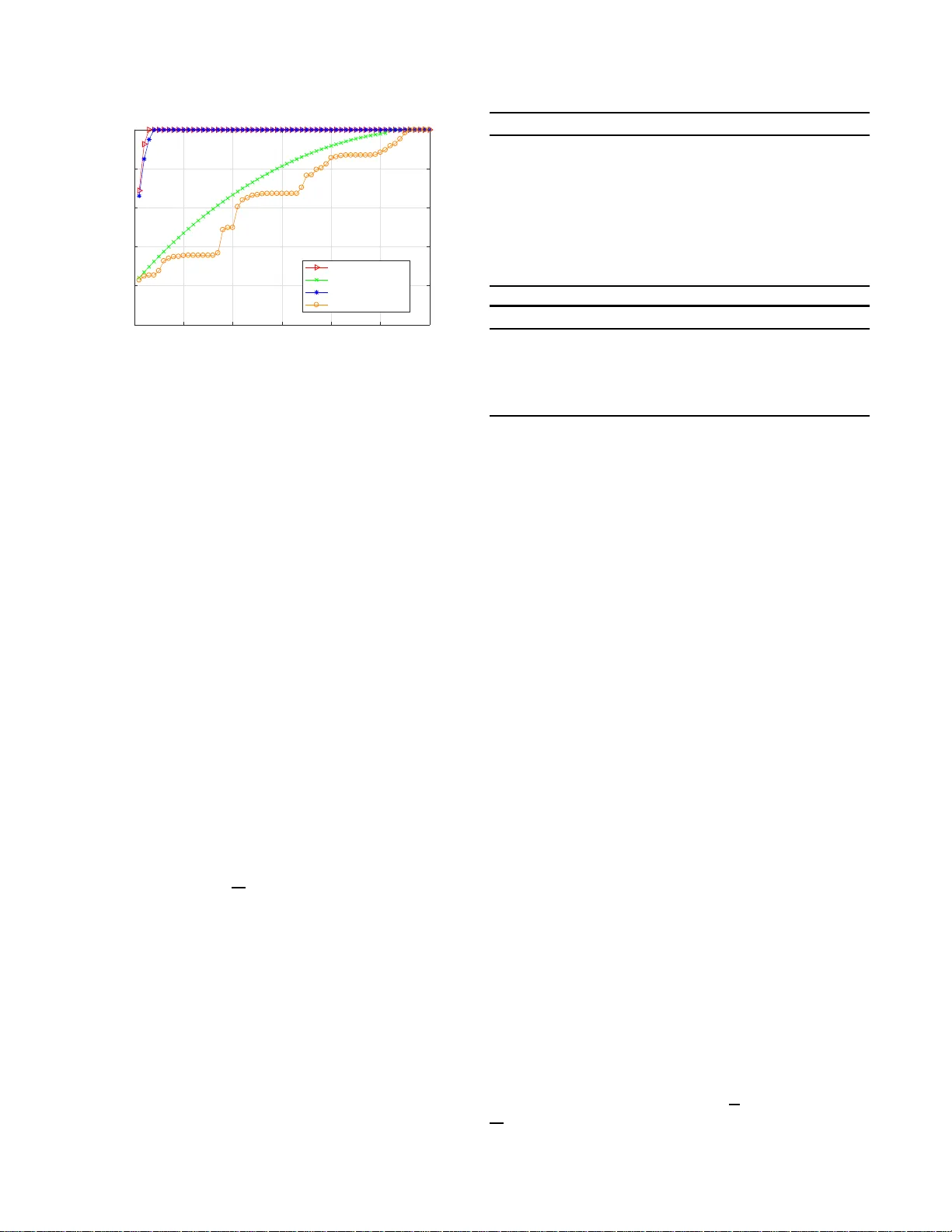
MUL TIDIMENSIONAL D A T A TENSOR SENSING FOR RF T OMOGRAPHIC IMA GING T ao Deng 1 , Xiao -Y ang Liu 2 , F eng Qian 1 and Anwar W alid 3 1 School of Comm unication and Information Engineering, Univ ersity of El ectronic Science and T echnology of China 2 Dept. of Electrical Engineering, Columbia Uni versity 3 Bell Laboratories ABSTRA CT Radio-freq uency ( RF) tomogr a phic imaging is a p romising technique for infe r ring multi-dim ensional physical space by processing RF sign a ls traversed across a region o f interest. Howe ver , conv entiona l RF tom ograp h y schemes are gen- erally based on vector co mpressed sensing, which ign ores the g eometric structures of the target spaces an d leads to low r ecovery p recision. The recently p ropo sed transform- based tensor model is mor e appr opriate for sensory data pro- cessing, as it help s exploit the geo metric structu res o f the three-dim ensional target and improve the recovery pr ecision. In this pap er , we prop ose a novel tensor sensing a pproac h that achieves highly accu rate estimation for real-world thr e e- dimensiona l spaces. First, we use the transform-ba sed ten- sor mod el to f ormulate a tensor sensing p roblem, and pro- pose a fast alter nating m inimization algorithm called Alt- Min. Secondly , we drive a n a lgorithm which is o ptimized to r educe memo ry and co mputation r equirem e nts. Finally , we present ev aluation of our Alt-Min approac h u sing IKEA 3D data and d emonstrate significant improvement in recovery error and con vergence speed compared to pr ior tensor-based compressed sensing. Index T erms — RF T omog raphic Imaging , T ransform - based T ensor, T ensor Sen sing, Alternating Minimization 1. INTR ODUCTION RF T omog raphic im aging [1, 2] is an infe r ence technique which can be used for remotely lear n ing th e lo c ations and the shapes of ob jects, as depicted in Fig. 1. RF tomograph ic imaging can be applied in smar t buildings and spaces app lica- tions [3], and in em ergencies, rescue operations a nd security breaches [4], since the ob jects being imag ed need not carry an electronic device or a cellphone. There h av e been considerable works on reconstructio n methods for RF tomo graph ic imaging which can be catego- rized into vector-based and tensor-based metho ds. In [1, 5 ], vector-based compressed sen sing approa c h es for RF to mo- graphic imaging are propo sed. These vector-based m ethods are design ed to infer two-d im ensional spaces, and they do not Fig. 1 : An illustration o f RF tomogr aphic imaging n etwork. Each node broad casts to the others, creatin g many projection s that can be u sed to reconstruct ob jects inside the network area . have the ability to estimate three- d imensional space s since spatial structures o f the d a ta a r e inherently igno red. Refer- ence [4] propo ses the tensor-based c ompressed sensing algo- rithm using tensor nuc le a r n orm (TNN) [6], which extends the RF to mograp hic imaging p roblem to th ree-dime nsional case. Ho wever , it requires computing te n sor singular value decomp o sition (t- SVD), which lea ds to h igh compu tational complexity , especially fo r large scale tensors. Moreover, the recovery er ror o f th is app roach is relatively high, an d the data size that can be h andled is to o small for realistic scenar ios. In this p aper, we aim to exp lo it the spatial structures of three- dimensiona l spaces fo r m ore efficient a nd accurate inference. In order to represent three-dimension al spa tial structures effecti vely , we adopt the recently prop osed transform- based tensor mo del [ 7], which has the following advantages: (i) compare d with other tensor m odels, only r eal-valued fast transform s are in volved, so it is appropriate f or the r e ceiv ed signal streng th (RSS) data; (ii) unlike other existing tensor models, th e tran sform-b ased tensor model allows f or diverse sampling strategies. On the other hand, we de compose the loss field tensor into the pr oduct of two tensors of sma ll sizes, so that we on ly need to iteratively u pdate two small tensors, which is much more effectiv e th a n prior tensor-based com- pressed sensing. In this pap er , we p ropose a novel RF tomo graph ic imag- ing scheme using tensor sensing to estimate th e three- dimensiona l spaces. W e f ormulate the RF tom ograp h ic ima g- ing as a tensor sensing pr oblem in a transfo rm domain, and propo se a novel Altern ating-Minim ization (Alt-Min) algo- rithm, whose implementatio n is op timized fo r memory con- sumption an d computatio n speed. W e app ly ou r algorithm to the IKEA 3D da tasets [8], and demon strate significantly lower recovery error a n d req uired nu mber of itera tions, com - pared with the appro ach in [4]. The rem a in der of the paper is organize d as follows: sys- tem model and pro blem fo rmulation are gi ven in Section II. Section III presents the solution a lgorithm, imp lementation and a lg orithm o ptimization. The ev aluation results are pre- sented in Section IV . Finally , we conclud e th is pap e r in Sec- tion V . 2. PR OBLEM ST A TEMENT AND FORMULA TION W e first revie w the RF tomogr aphic ima g ing problem [1, 3, 9], then m o del the shadowing lo ss data as a transform-ba sed tensor, and f ormulate the RF tomograph ic imaging task as a tensor sensing prob lem. Notatio ns- W e use lowercase bold face letter x ∈ R N 1 to d e- note a vector , up p ercase bo ldface letter X ∈ R N 1 × N 2 to de- note a matrix , and calligrap hic letter X ∈ R N 1 × N 2 × N 3 to denote a tensor . Let [ k ] denote the set { 1 , 2 , · · · , k } . 2.1. RF T omographic Channel Model W e consider the RF tomograph ic imaging with the space of interest be in g repre sen ted as a 3D tensor in Cartesian coor- dinates. A set of RF signal nodes are unifor mly deployed around the sides of the “tensor” , fo rming a comp le te tomog - raphy network. Any pair of nodes can establish a un ique link. The RF sign a l on a given link suf fers f rom path lo ss, which consists of three parts: (i) shadowing loss due to obstruc- tions; (ii) distant-depen dent large-scale path loss; (iii) non - shadowing loss due to mu ltipath [1]. W e use V to re present the no d e set, and assum e that v i ∈ V is a tra n smitter and v j ∈ V ( i 6 = j ) is a receiver . Let P ij be the recei ved power at v j , then we can o btain the following p ower equation: P ij = P t − P ( d ij ) − Z ij , Z ij = Z (1) ij + Z (2) ij , (1) where P t is th e tran smitted power , d ij is th e distanc e be- tween node v i and v j , an d P ( d ij ) represen ts the co rrespond - ing large-scale path loss of the link . Let Z ij be the total fading loss that in volves the non-shad owing fading loss Z (2) ij and the shadowing loss Z (1) ij . Assuming tha t the spac e of intere st X ∈ R N 1 × N 2 × N 3 is divided into a set of three- dimension al voxels of the same size. W e use ∆( n 1 , n 2 , n 3 ) ∈ R 3 ( n 1 ∈ [ N 1 ] , n 2 ∈ [ N 2 ] , n 3 ∈ [ N 3 ]) to denote a voxel at the co r respond ing coo r di- nate. When the RF signal pro pagates thro ugh th e voxels , the total value of shad owing loss Z (1) ij is equiv alent to the total attenuation that ar ises in each single voxel. Mo reover , we assume th at the intern al med ium of each voxel is homo- geneou s, and the power attenua tio n coefficient is a constant value X ( n 1 , n 2 , n 3 ) within ∆( n 1 , n 2 , n 3 ) [4]. Gi ven th ese definitions, the shadowing loss o f a unique link ( i, j ) between v i and v j can be form ulated as: Z (1) ij = X n 1 ,n 2 ,n 3 D ij ( n 1 , n 2 , n 3 ) X ( n 1 , n 2 , n 3 ) , (2) where D ij ( n 1 , n 2 , n 3 ) represen ts the overlapped distance be- tween the link ( i, j ) and voxel ∆( n 1 , n 2 , n 3 ) . The non- shadowing fading loss Z (2) ij is assumed to be a stationary Gaussian process with zero m ean and variance σ 2 [4]. 2.2. T ra nsform-based T ensor Model Let A ∈ R N 1 × N 2 × N 3 denote a third-ord er tensor . A (: , j, k ) , A ( i, : , k ) , A ( i, j, :) d enote mode-1 , m ode-2, mode- 3 tubes of A , and A (: , : , k ) , A (: , j, :) , A ( i, : , :) den o te the frontal, lat- eral, an d horizontal slices. The Froben ius no rm of A is de- fined as kAk F = q P N 1 i =1 P N 2 j =1 P N 3 k =1 A 2 ij k . The op erator vec( · ) transfo rms tensors and matrices into vector s. Let X T and A † denote the transposes of a m atrix and a tenso r , respec- ti vely . Definition 1. [7] Given an invertible discr ete transform L : R 1 × 1 × N 3 → R 1 × 1 × N 3 , the elemen twise multiplica tio n ◦ , and a , b ∈ R 1 × 1 × N 3 , th e tuba l-scalar multiplication is defi n ed as a • b = L − 1 ( L ( a ) ◦ L ( b )) , (3) wher e L − 1 is the in verse of L . Definition 2. [7] The L -pr oduct A = B • C of B ∈ R N 1 × r × N 3 and C ∈ R r × N 2 × N 3 is a tensor of size N 1 × N 2 × N 3 , A ( i, j, :) = P r s =0 B ( i, s, :) • C ( s, j, :) , for i ∈ [ N 1 ] and j ∈ [ N 2 ] . Definition 3 . [7] The transpose of A , A † ∈ R N 2 × N 1 × N 3 satisfies L  A †  ( i ) =  L ( A ) ( i )  T , i ∈ [ N 3 ] . Definition 4. [7] Identity tensor b ased on L -pr oduct is de- fined a s I ∈ R N 1 × N 1 × N 2 with L ( I ) ( i ) , i ∈ [ N 2 ] ar e N 1 × N 1 identity matrices. Definition 5. [7 ] A is L -orthogon al if A • A † = A † • A = I . Definition 6. [7] The transform d omain singu lar value de- composition L -SVD of A ∈ R N 1 × N 2 × N 3 is given by A = U • S • V † , wher e U and V ar e L -orthogo nal tensors of size N 1 × N 1 × N 3 and N 2 × N 2 × N 3 r espectively , and S is a diagonal tenso r of size N 1 × N 2 × N 3 . Th e en tries of S ar e called the singular values of A , and the nu mber of no n-zer o ones is called the L -rank of A . 0 10 20 30 40 50 60 Number of Singular Values 0 20 40 60 80 100 Percentage (%) Empirical CDF L-SVD with FFT Matrix-SVD L-SVD with DCT CP-Decomposition Fig. 2 : Th e CDFs of singular values of L -SVD with FFT , L -SVD with DCT , matrix -SVD a n d CP-Decompo sition. In order to verif y the validity o f the m odel, we use an IKEA 3D chair model to generate a g round truth tensor o f size 60 × 60 × 15 ( details are g iv en in Section 4.1), then the tensor is tr ansformed to its frequ ency domain b y fas t fourier tr ans- formation (FFT) and discrete cosine transfo rmation (DCT). Fig. 2 shows the empirical cu mulative distribution function (CDF) of th e tensor singu lar values. For L -SVD with FFT , 3 out of 60 singular values cap ture 95% of the energy , while the correspond ing number of sing ular values are 3 8 an d 54 for matrix- SVD and traditional tensor CP-Deco mposition, re- spectiv ely . For L -SVD with DCT , 4 singular values ca p- ture 95% energy . Therefo re, th e low L -ran k p roper ty of transform -based ten sor mo del is more appropriate for the RF tomogr a phy imagin g pr oblem than other metho d s; a similar conclusion is giv en in the context of fingerpr int loc alization [10]. 2.3. Problem Formulation Let K be the number of nodes within the n etwork, then the total numb er of two-way links we can obtain is S = ( K 2 − K ) / 2 . Assuming tha t we imp lement M (1 ≤ M ≤ S ) times measuremen ts, and each measuremen t in volves a unique link . Those M n o des p airs are indexed as ( v i m , v j m ) , m ∈ [ M ] . W e obtain the following linear m easuremen t: y m = P t − P i m j m − P ( d i m ,j m ) = X n 1 ,n 2 ,n 3 D i m j m ( n 1 , n 2 , n 3 ) X ( n 1 , n 2 , n 3 ) + Z (2) i m j m , (4) where y m is refe rred to as th e m - th measur ed total fading loss. Then we stack these RF signal measurements y m into a mea su rement vector y ∈ R M [11]. Giv en linear measure- ments y m = hX , A m i = ( vec ( A m )) T · vec ( X ) , 1 ≤ m ≤ M of a loss field tensor X ∈ R N 1 × N 2 × N 3 with L - rank r and the sensing tensor s A m ∈ R N 1 × N 2 × N 3 . W ith a lin ear map H ( · ) : R N 1 × N 2 × N 3 → R M [12], (4) is rewritten as f ollows: y = H ( X ) + w , (5) Algorithm 1 Alt-Min: AM( H ( · ) , y , r, L ) Input: linear map H ( · ) , measureme n t vector y , L -ran k r , iteration number L . 1: Initialize U 0 random ly; 2: for ℓ = 1 to L do 3: V ℓ ← L S ( H ( · ) , U ℓ − 1 , y , r ) ; 4: U ℓ ← LS( H ( · ) , V ℓ , y , r ) ; 5: end for Output: Pair of tensors ( U L , V L ) . Algorithm 2 Least Square s Minim ization: LS( H ( · ) , U , y , r ) Input: linear map H ( · ) , tensor U ∈ R N 1 × r × N 3 , measure- ment vector y , L -rank r . 1: V = arg min V ∈ R r × N 2 × N 3 k y − H ( U • V ) k 2 F ; Output: tensor V where w = ( Z (2) i 1 j 1 , Z (2) i 2 j 2 , · · · , Z (2) i M j M ) T denotes the noise vector . The goal of RF tomogr aphic imaging is to recover the loss field tensor X from th e measuremen t vector y . W e form ulate this problem as a low L -rank tensor sensing prob lem: b X = arg min X ∈ R N 1 × N 2 × N 3 k y − H ( X ) k 2 F , s.t. rank( X ) ≤ r. (6) 3. SOLUTION ALGO RITHM VIA AL T -MIN In this section, we present a novel iter ativ e algorithm , called Alt-Min, and revie w its optimizatio n and imp lementation . 3.1. The Alt-Min Alg orithm T o enable alternating minim ization, we re present the loss field ten sor as the L -produ c t of two smaller ten sors [ 13], i.e., X = U • V , X ∈ R N 1 × N 2 × N 3 , U ∈ R N 1 × r × N 3 and V ∈ R r × N 2 × N 3 . Then we refor mulate e quation (6) as the following non- conv ex o ptimization prob lem: b X = arg min U ∈ R N 1 × r × N 3 , V ∈ R r × N 2 × N 3 k y − H ( U • V ) k 2 F . (7) The main idea of Alt-Min is to iter ativ ely estimate two low L -rank tensors U and V , each of L -ra nk r . The key step is least squares (LS) minim ization ( see Alg . 2 ). The d etailed implementatio n of LS min im ization are given below . W e ad opt circulan t algebra [1 3, 14] to extend matrix alge- bra to third -order ten sors. A tubal scalar rep resents a vector of length N 3 , and the correspo nding space is d enoted as K . L et K N 1 × N 2 denote the space of N 1 × N 2 tubal matric e s where each elemen t is a tu bal scalar in K . Let α be a tubal scalar, and A be a tubal matrix. W e use the oper a tor circ ( · ) [14] to m ap circulants to their c orrespon ding circular matrices, which are tagged with the superscrip t c , i.e., α c , A c : α c = circ ( α ) =      α 1 α N 3 · · · α 2 α 2 α 1 · · · · · · . . . . . . . . . α N 3 α N 3 α N 3 − 1 · · · α 1      , A c = circ ( A ) =    circ ( A 1 , 1 ) · · · circ ( A 1 ,N 2 ) . . . . . . . . . circ ( A N 1 , 1 ) · · · circ ( A N 1 ,N 2 )    . For simplicity , we use A c to repr esent the circular ma tr ix of tensor A . Then the L -prod uct X = U • V has an e q uiv alent matrix-pr oduct as: X c = U c V c , (8) where X c ∈ R N 1 N 3 × N 2 N 3 , U c ∈ R N 1 N 3 × r N 3 , V c ∈ R r N 3 × N 2 N 3 . W e can transform the LS minimization in Alg. 2 to the corresp o nding circ ular matrix represen tation: b V c = arg min V c ∈ R rN 3 × N 2 N 3 k y − H c ( U c V c ) k 2 F , (9) where H c ( · ) : R N 1 N 3 × N 2 N 3 → R M is the co rrespond - ing linear map in the cir cular matrix repre sen tation, with y = H c ( X c ) . Each sensing tensor A m is tr a n sformed into its circular ma tr ix A c m ∈ R N 1 N 3 × N 2 N 3 , and y m = h X c , A c m i , 1 ≤ m ≤ M . Similarly , we can e stima te U c in the following way: b U c = arg min U c ∈ R N 1 N 3 × rN 3    y − H c T ( V c T U c T )    2 F . (1 0) W e perfor m the following steps to solve this non-conve x optimization problem : Step 1) . U c is used to form a b lo ck diagon al m a trix B 1 of size N 1 N 2 N 2 3 × r N 2 N 2 3 , and th e n umber of U c is N 2 N 3 , B 1 =      U c U c . . . U c      . (11) Step 2 ) . Stack all the colu m ns of V c , and then V c is vectorized to a vector b o f size rN 2 N 2 3 × 1 as fo llows: b = vec ( V c ) = [ V c (: , 1) T , V c (: , 2) T , . . . , V c (: , N 2 N 3 ) T ] T . (12) Step 3) . Each A c m , 1 ≤ m ≤ M is represen te d as a vector c m of size N 1 N 2 N 2 3 × 1 in the f o llowing way: c m = vec ( A c m ) = [ A c m (: , 1) T , A c m (: , 2) T , . . . , A c m (: , N 2 N 3 ) T ] T , (13) and then all the c m are transform e d into a m a tr ix B 2 of size M × N 1 N 2 N 2 3 : B 2 = [ c 1 , c 2 , . . . , c M ] T . (14) Therefo re, the estimation of V c is transformed in to the following standard least squ a res minimization prob lem: b b = a r g min b ∈ R rN 2 N 2 3 × 1 k y − B 2 B 1 b k 2 F . (15) 3.2. Algorit hm Optimization The prop osed Alt-Min requ ires large m emory consum ption and high co mputatio n al-comp lexity . W e prop ose improve- ments to resolve su ch prob lems. 3.2.1. Optimization o f Alt-Min As stated above, the loss field tensor and the sensing tensor are transformed to an unkn own circular ma trix X c ∈ R N 1 N 3 × N 2 N 3 and a sensing circular matrix A c m ∈ R N 1 N 3 × N 2 N 3 , respectively . The unk nown circular matrix X c consists of N 1 N 2 N 2 3 entries and if we set the samp lin g r ate as 5 0%, the total n u mber o f all sensing circu lar ma tr ices is 0.5 N 1 N 2 N 2 3 . In this case, the space co mplexity of all sensing matrices is O ( N 2 1 N 2 2 N 4 3 ) , and it is obvious that the memor y requirem ent increases exponentially with the size o f the ten - sor . T o alle viate this p roblem, we p r opose a mod ified versio n of the impleme n tation. In circu lant algebra, it is obvious that the first co lumn of α c already contains all the entries of itself, and there is no need to recover the redu ndant information . For recovering the loss field tensor X , we on ly need to recover th e first column of each circ ( X i,j ) , which we set as the i -th tube of the j -th lateral slice: X ( i, j, :) . W e use the Matlab function squeeze ( · ) to get a new definition: X s =    squeeze ( X (1 , 1 , :)) · · · squeeze ( X (1 , N 2 , :)) . . . . . . . . . squeeze ( X ( N 1 , 1 , :)) · · · squeeze ( X ( N 1 , N 2 , :))    , where squeeze ( X ( i, j, :)) transforms th e i -th tube o f the j -th lateral slice of X into a vector of size N 3 × 1 . W e use the notation ⇔ to denote a new m apping for L - produ ct as follows: X = U • V ⇔ X s = U c V s , (16) where X s ∈ R N 1 N 3 × N 2 , U c ∈ R N 1 N 3 × r N 3 , V s ∈ R r N 3 × N 2 . W e c a n transfo rm the LS minimization in A lg . 2 to the following r epresentation : b V s = arg min V s ∈ R rN 3 × N 2 k y − H s ( U c V s ) k 2 F , (17) (a) (b) (c) (d) Fig. 3 : (a) an d (c) are the 3D v isu a lizations of two IKEA models, (b) and ( d) are the correspo nding rec overy results. where H s ( · ) : R N 1 N 3 × N 2 → R M is the correspond ing linear map, with y = H s ( X s ) , y m = h X s , A s m i , 1 ≤ m ≤ M . Similarly , we can estimate U c in the fo llowing way: b U c = ar g min U c ∈ R N 1 N 3 × rN 3    y − H s T ( V s T U c T )    2 F . (18) 3.2.2. Complexity A nalysis As stated above, if we use 50% sampling rate, the original s pace complexity is O ( N 2 1 N 2 2 N 4 3 ) . In the modified version, we transform X , A m to X s ∈ R N 1 N 3 × N 2 , A s m ∈ R N 1 N 3 × N 2 , and the space complexity de- creases to O ( N 2 1 N 2 2 N 2 3 ) , wh ich is 1 / N 2 3 of the fo rmer value. Note that we only calcu late the reduction of space complex- ity for the sensing matrices, but there are addition ally large reduction in inter mediate variables. Therefo re, the above al- gorithm o ptimization is a key enabler in our appro a ch for in- ferring large thre e -dimension al phy sical space. 4. PERFORMANCE EV ALU A TION 4.1. Data Sets And Model V erificatio n W e compar e the pr oposed algorithm Alt-M in with tenso r- based compr e ssed sensin g [ 4] on the IKEA 3D datasets. W e adopt an IKEA 3D ch air m odel and tab le mod el to generate two groun d truth tensor s of th e sam e size 60 × 60 × 15 . The L -rank of the chair model is 3, and that of the table model is 4. E ach 3D m o del is placed in the middle of the “ten sor” and occupies a par t of the space. In this task, we mainly focus on the loc ation and outline information , while th e texture and color informa tion are ign ored. 4.2. Algorit hm Comparison Metrics W e comp are the Alt-Min a g ainst the re cently prop osed tensor- based compr essed sensing [4] on the IKEA 3D d atasets. Note that we carry out two versions of the Alt-Min: Alt-M in with FFT an d Alt-M in with DCT . The tensor-based c ompressed sensing uses TNN as the regularization, in which th e t-SVD is condu c te d in every iteration. Our alg orithm is based on th e bi- linear factorization, and we only need to iteratively upd ate the two smaller tensors. For quantitative co mparison, we adopt two m etrics: the recovery error and the conver gence speed. • For r e covery e r ror, we u se th e m e tric relative square error, defined as RSE = || b X − X || F / ||X || F . • For the convergence sp e e d, we linear ly fitting the mea- sured RSEs across iteration s, and then compar e th e d e- creasing rate of eac h method. 4.3. Perf ormance Results Fig. 3 shows the 3D visualizatio ns of an IKEA chair, an IKEA table, and our correspond in g recovery results using Alt-Min with DCT . For all methods, we use 50% samplin g r ate, and the maximum iteration number is set to 20. The final recovery error (RSE in log -scale) o f the chair mo del is 10 − 8 in mag- nitude, a n d that of the table model is 10 − 7 . W e can ob serve that Alt-M in with DCT successfu lly recovers th e outlines of two mod e ls. Note that we focus on the outline s o f the mod- els instead of the whole space, and the r ecovery results are artificially coloured for a b etter visualization . Th e following analysis is based on th e expe r iments of th e ch air model. T o examine recovery er ror perform ance, we fix the max - imum iteration numbers o f three methods to be 2 0. Then we vary the samplin g rate from 20% to 80% by selecting wire- less links randomly [ 15]. Each sampling rate is measured 5 times, and the a verage rec overy er ror results are compu ted. Fig. 4 depicts the RSEs of Alt-Min with FFT , Alt-Min with DCT and tensor-based compressed sensing for varying sam- pling rates. For low sampling rates ( 20% ∼ 25%), tensor- based comp r essed sensing perfo rms better than Alt-M in with FFT and Alt-Min with DCT . For sampling rates varying from 30% to 80%, the RSEs of two Alt-Min me thods decrease significantly , while that of tensor -based compressed sensing decreases very slowly . For 80% sampling ra te, th e RSE of Alt-Min with FFT is aro und 10 − 13 in m agnitud e , and that of Alt-Min with DCT is a little high er , while the th e RSE of tensor-based comp ressed sensing is at arou nd 1 0 − 3 . Fig. 5 an d Fig. 6 show the co nvergence rates o f Alt-Min with FFT and with DCT , r espectively . The sampling rate is fixed to be 50% , the maximu m iteration number is set at 30. 20 30 40 50 60 70 80 Sampling Rate (x 100%) 10 -14 10 -12 10 -10 10 -8 10 -6 10 -4 10 -2 10 0 10 2 RSE in log-scale Alt-Min with FFT Alt-Min with DCT Tensor-based CS Fig. 4 : RSEs vs samp ling rates. 0 5 10 15 20 25 30 Iterations (No.) -12 -10 -8 -6 -4 -2 0 RSE in log-scale Linear Equation: y=-0.354*x - 0.272 Fig. 5 : Alt-Min with FFT . 0 5 10 15 20 25 30 Iterations (No.) -12 -10 -8 -6 -4 -2 0 RSE in log-scale Linear Equation: y=-0.359*x - 0.408 Fig. 6 : Alt-Min with DCT . A linear fit to the data is also shown. Note that if we set the RSE th reshold to be 10 − 10 , we only n eed approximately 27 iterations for both method s. 5. CONCLUSION In this paper, we use the tr ansform- based tensor mod el to for- mulate the RF tom ograp hic im aging as a te n sor sensing prob- lem, which can fully exp lo it the geome tric structures of the three-dim ensional loss field tensor . The n we pro pose a fast iterativ e alg orithm Alt-Min for the low L -rank tensor sens- ing. The loss field ten so r is factorized as the L -product of two smaller ten so rs, and then Alt-Min alternately estimates those two tensor s by LS minimiza tio n. The ev aluation results on IKEA 3 D datasets h av e demon strated that Alt-Min signif - icantly imp roves the recovery error an d convergence speed compare d to prior tensor-based compressed sensing. 6. REFERENCES [1] M.A. Kanso and M.G. Rabb a t, “Compr essed RF tomog - raphy for wireless sensor networks: Centralized and de- centralized app roaches, ” in Int. Con. D istributed Com- puting in Se n sor S ystems . Spring er , 20 0 9, pp . 173– 1 86. [2] A. Liutkus, D. Martina, S. Po poff, and etc., “Ima g ing with natur e: compressive imaging using a multiply scat- tering mediu m, ” Scientific Reports , vol. 4, 2 014. [3] J. Wilson and N. P atwari, “Radio tomo graph ic imaging with wireless networks, ” IEEE T ransactions on Mobile Computing , vol. 9, no. 5, pp. 62 1–632 , 2010. [4] T . Matsuda, K. Y okota, K. T akemoto , S. Hara, F . Ono, K. T akizawa, and R. Miura, “Multi-d imensional wir e- less tomog raphy using tensor-based compressed sens- ing, ” W ir eless P ersonal Communications , vol. 9 6, no. 3, pp. 336 1–33 8 4, 2017. [5] Y . Mostofi, “Compressive cooperative sensing an d m ap- ping in mobile networks, ” IEEE T ransactions on Mo bile Computing , vol. 10, no. 12, pp. 17 69–17 84, 2011. [6] Q. Li, D. Schon feld, an d S. Friedland, “Generalized tensor compressive sensing, ” in IEEE Int. Con. o n Mul- timedia and Expo (ICME) . IE E E, 2013, pp. 1–6. [7] X.-Y . Liu and X. W ang , “Fourth-or der tensors with multidimen sio n al discrete transforms, ” arXiv pr eprint arXiv:170 5.015 76 , 2 017. [8] Joseph J.L., Hamed P ., and Antonio T ., “Parsing IKEA objects: fine pose estimation, ” In ternationa l Confer ence on Computer V ision , 20 13. [9] F . Ad ib, Z. K a belac, D. Katabi, and R.C. Miller, “3D tracking via bod y radio reflection s, ” in Networked sys- tems Design an d Implementation , 201 4, vol. 14, pp. 317–3 29. [10] X.-Y . Liu, S. Aero n, V . Aggarwal, X. W ang , and M.- Y . W u, “ Ada ptiv e sampling of RF fingerprin ts for fine- grained indoo r lo calization, ” IEEE T ransactions on Mo- bile Computing , vol. 15 , no. 10, pp. 2 411– 2 423, 2016 . [11] L. Kong, M. Xia, X.- Y . Liu, G. Chen, Y . Gu, M.- Y . W u, and X. Liu, “Data loss a n d re construction in wireless sensor n etworks, ” IE E E T r ansactio ns on P arallel an d Distrib uted Systems , vol. 25, no . 11, pp. 2818 –282 8, 2014. [12] P . Jain, P . Netrapalli, a n d S. Sanghavi, “Low-rank matr ix completion u sing alternating minim ization, ” in Pr oc. AC M symposium on Theory of Compu ting . ACM, 20 13, pp. 665–6 74. [13] X.-Y . Liu, S. Aero n , V . Agg arwal, an d X. W an g, “Low- tubal-ran k tensor completion using alternating mini- mization, ” arXiv pr eprint arXiv:16 1 0.016 90 , 2 016. [14] D.F . Gleich, C. Greif, a n d J.M. V arah, “The power and arnoldi metho d s in an algebra of cir culants, ” Numeri- cal Lin ear Algebra with Application s , vol. 20, no. 5, pp. 809–8 31, 201 3. [15] X.-Y . Liu, Y . Zh u, L. K ong, C. Liu, Y . Gu, A . V . V asi- lakos, and M.-Y . W u , “Cdc: Compressiv e d ata co llec- tion for wireless sensor networks, ” IEE E T ransactions on P arallel and Distributed Systems , vol. 26, no . 8, pp. 2188– 2197 , 20 15.