The Partially Observable Hidden Markov Model and its Application to Keystroke Dynamics

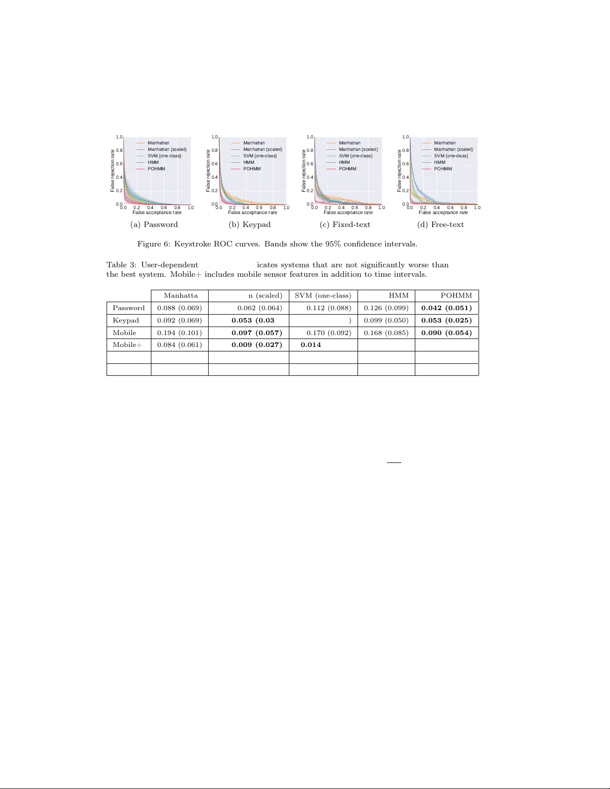
The P artially Observ able Hidden Mark o v Mo del and its Application to Keystrok e Dynamics John V. Monaco a, ∗ , Charles C. T appert b a U.S. Army R ese ar ch L ab oratory, A b er deen Pr oving Gr ound, MD 21005, USA b Pac e University, Ple asantvil le, NY 10570, USA Abstract The partially observ able hidden Marko v mo del is an extension of the hidden Mark ov Model in which the hidden state is conditioned on an independent Mark ov c hain. This structure is motiv ated by the presence of discrete metadata, suc h as an even t type, that ma y partially rev eal the hidden state but itself emanates from a separate pro cess. Suc h a scenario is encoun tered in k eystroke dynamics whereb y a user’s t yping b eha vior is dep enden t on the text that is t yp ed. Under the assumption that the user can b e in either an active or passive state of typing, the keyboard key names are even t t yp es that partially rev eal the hidden state due to the presence of relatively longer time in terv als b et ween w ords and sen tences than b et ween letters of a word. Using ﬁv e public datasets, the prop osed mo del is shown to consistently outp erform other anomaly detectors, including the standard HMM, in biometric identiﬁcation and veriﬁcation tasks and is generally preferred ov er the HMM in a Monte Carlo go o dness of ﬁt test. Keywor ds: hidden Mark ov mo del, keystrok e biometrics, b eha vioral biometrics, time in terv als, anomaly detection 1. In tro duction The hidden Marko v mo del (HMM), which dates back ov er 50 y ears [1], has seen numerous applications in the recognition of human b ehavior, such as sp eec h [2], gesture [3], and handwriting [4]. Recent successes ha ve leveraged the expres- siv e p o w er of connectionist mo dels by combining the HMM with feed-forward deep neural net w orks, which are used to estimate emission probabilities [5, 6, 7]. Despite the increasing in terest in sequen tial deep learning techniques, e.g., re- curren t neural netw orks, HMMs remain tried-and-true for time series analyses. The p opularity and endurance of the HMM can b e at least partially attributed ∗ Corresponding author Email addr ess: john.v.monaco2.civ@mail.mil (John V. Monaco) URL: http://www.vmonaco.com (John V. Monaco) Pattern R e c ognition (ac c epte d manuscript) Novemb er 21, 2017 2 to the tractability of core problems (parameter estimation and lik eliho o d calcu- lation), ability to b e combined with other metho ds, and the level of insight it pro vides to the data. A t least part its success can also b e attributed to its ﬂexibility , with man y HMM v arian ts ha ving b een developed for sp eciﬁc applications. This usually in volv es in tro ducing a dep endence, whether it b e on time [8], previous obser- v ations [9], or a semantic context [10]. The motiv ation for doing so is often to b etter reﬂect the structure of the underlying problem. Although man y of these v ariations hav e increased complexity and num ber of parameters ov er the standard HMM, their estimation remains tractable. In this work, w e introduce the partially observ able hidden Mark ov mo del (POHMM), an extension of the HMM in tended for keystrok e dynamics. W e are in terested in mo deling the temp oral b ehavior of a user typing on a keyboard, and note that certain keyboard keys are thought to inﬂuence typing sp eed. Non- letter keys, such as punctuation and the Space key , indicate a greater probability of b eing in a p assive state of typing, as opp osed to an active state, since the t ypist often pauses b etw een w ords and sen tences as opp osed to b et ween letters in a word [11]. The POHMM reﬂects this scenario b y introducing a dep endency on the key names whic h are observed alongside the time interv als, and in this w ay , the keys provide a context for the time in terv als. The idea of introducing a context up on whic h some behavior dep ends is not new. Often, an observ ation depends not only on a latent v ariable but on the observ ations that preceded it. F or example, the neigh b oring elements in a protein secondary structure can pro vide con text for the element under consideration, which is though t to dep end on both the previous element and a hidden state [9]; nearby phonemes can aid in the recognition of phonemes [12]; and the recognition of h uman activities can b e achiev ed with greater accuracy b y considering b oth a spatial con text (e.g., where the activity o ccurred) and temp oral context (e.g., the duration of the activity) [13]. Handwriting recognition has generally seen increased p erformance with mo d- els that consider the surrounding context of a handwritten character. The ra- tionale for suc h an approach is that a character ma y b e written with diﬀeren t st yle or strok es dep ending on its neighboring c haracters in the sequence. Un- der this assumption, the neighboring pixels or feature vectors of neighboring c haracters can provide additional context for the c haracter under consideration. Alternativ ely , a separate mo del can be trained for each context in whic h the c haracter app ears, e.g., “t” follow ed by “e” versus “t” follow ed b y “h” [10]. This same principle motiv ates the developmen t of the POHMM, with the diﬀerence b eing that the con text is provided not b y the observ ations themselves, but b y a separate sequence. W e apply the POHMM to address the problems of user iden tiﬁcation, veri- ﬁcation, and contin uous v eriﬁcation, leveraging keystrok e dynamics as a b ehav- ioral biometric. Eac h of these problems requires estimating the POHMM pa- rameters for each individual user. Iden tiﬁcation is p erformed with the maximum a p osteriori (MAP) approach, choosing the mo del with maximum a p osterior probabilit y; v eriﬁcation, a binary classiﬁcation problem, is achiev ed b y using 3 the model log-lik eliho od as a biometric score; and con tin uous v eriﬁcation is ac hieved b y accum ulating the scores within a sliding window ov er the sequence. Ev aluated on ﬁve public datasets, the prop osed mo del is shown to consisten tly outp erform other leading anomaly detectors, including the standard HMM, in biometric iden tiﬁcation and v eriﬁcation tasks and is generally preferred o ver the HMM in a Mon te Carlo go o dness of ﬁt test. All of the core HMM problems remain tractable for the POHMM, includ- ing parameter estimation, hidden state prediction, and likelihoo d calculation. Ho wev er, the dep endency on even t types in tro duces many more parameters to the POHMM than its HMM counterpart. Therefore, we address the problem of parameter smo othing, which acts as a kind of regularization and av oids ov erﬁt- ting [14]. In doing so, we deriv e explicit marginal distributions, with ev ent t yp e marginalized out, and demonstrate the equiv alence b etw een the marginalized POHMM and the standard HMM. The marginal distributions con venien tly act as a kind of back oﬀ, or fallback, mechanism in case of missing data, a technique ro oted in linguistics [15]. The rest of this article is organized as follo ws. Section 2 brieﬂy describ es k eystroke dynamics as a b eha vioral biometric. Section 3 introduces the POHMM, follo wed b y a simulation study in Section 4 and a case study of the POHMM applied to k eystroke dynamics in Section 5. Section 6 reviews previous mo deling eﬀorts for latent pro cesses with partial observ ability and contains a di scussion. Finally , Section 7 concludes the article. The POHMM is implemen ted in the pohmm Python pac k age and source co de is publicly av ailable 1 . 2. Keystrok e dynamics Keystrok e dynamics refers to the wa y a p erson t yp es. Prominen tly , this includes the timings of key press and release even ts, where each k eystroke is comprised of a press time t n and a duration d n . The time in terv al b et ween k ey presses, τ n = t n − t n − 1 , is of interest. Compared to random time interv als (R TIs) in which a user presses only a single key [16], key press time interv als o ccur b etw een diﬀerent keys and are thought to be dep enden t on key distance [11]. A user’s k eystroke dynamics is also thought to b e relativ ely unique to the user, which enable biometric applications, suc h as user identiﬁcation and v eriﬁcation [17]. As a b eha vioral biometric, k eystrok e dynamics enables low-cost and non- in trusive user iden tiﬁcation and veriﬁcation. Keystroke dynamics-based veriﬁ- cation can b e deploy ed remotely , often as a second factor to username-password v eriﬁcation. Some of the same attributes that make keystrok e dynamics at- tractiv e as a b eha vioral biometric also presen t priv acy concerns [18], as there exist n umerous metho ds of detecting k eystrokes without running softw are on the victim’s computer. Recently , it has b een demonstrated that keystrok es can 1 A v ailable at https://gith ub.com/vmonaco/p ohmm and through PyPI. 4 b e detected through a wide range of mo dalities including motion [19], acoustics [20], net work traﬃc [21], and even WiFi signal distortion [22]. Due to the keyboard b eing one of the primary h uman-computer interfaces, it is also natural to consider k eystrok e dynamics as a modality for c ontinu- ous veriﬁc ation in which a v eriﬁcation decision is made up on each k ey pressed throughout a session [23]. Con tin uous veriﬁcation holds the promise of greater securit y , as users are veriﬁed contin uously throughout a session b ey ond the ini- tial login, which is considered a form of static veriﬁc ation . Being a sequential mo del, the POHMM is straightforw ard to use for contin uous veriﬁcation in ad- dition to iden tiﬁcation and static veriﬁcation. Keystrok e time interv als emanate from a combination of physiology (e.g., age, gender, and handedness [24]), motor b eha vior (e.g., typing skill [11]), and higher-lev el cognitive pro cesses [25], highligh ting the diﬃculty in capturing a user’s typing b ehavior in a succinct mo del. Typing behavior generally ev olves o ver time, with highly-practiced sequences able to b e t yp ed muc h quick er [26]. In biometrics, this is referred to as template aging . A user’s keystrok e dynamics is also generally dep endent on the typing task. F or example, the time interv als observ ed during passw ord entry are m uch diﬀerent than those observed during email comp osition. 3. P artially observ able hidden Marko v mo del The POHMM is in tended for applications in which a sequence of event typ es pro vides context for an observed sequence of time intervals . This reasoning extends activities other than keystrok e dynamics, such as email, in whic h a user might b e more lik ely to tak e an extended break after sending an email instead of receiving an email, and programming, in whic h a user ma y ﬁx bugs quic ker than making feature additions. The even ts types form an indep endent Mark ov chain and are observed alongside the sequence of time in terv als. This is in contrast to HMM v ariants where the neigh b oring observ ations themselves pro vide a context, such as the adjacent characters in a handwritten segment [10]. Instead, the even t t yp es are indep enden t of the dynamics of the mo del. With this structure, a distinction can b e made b etw een user b ehavior and task : the time in terv als comprise the b ehavior , and the sequence of even t t yp es, (e.g., the k eys pressed) comprise the task. While the time interv als reﬂect how the user behav es, the sequence of even ts c haracterize what the user is doing. This distinction is appropriate for keystrok e dynamics, in which the aim is to capture typing b ehavior but not the text itself whic h may more appropriately mo deled by linguistic analysis. Alternativ ely , in case the user transcrib es a sequence, such as in typing a password, the task is clearly deﬁned, i.e. the user is instructed to type a particular sequence of characters. The POHMM aims to capture the temp oral b ehavior, which dep ends on the task. 3.1. Description The HMM is a ﬁnite-state mo del in which observ ed v alues at time t dep end on an underlying latent pro cess [2]. At the n th time step t n , a feature vector 3.1 Description 5 z 1 z 2 z N − 1 z N ω 1 ω 2 ω N − 1 ω N 0 1 2 N − 1 N x 1 x 2 x N − 1 x N Eve n t t yp e (o b se rve d ) S t a t e (h i d d e n ) Emi ssi o n ( o b se rve d ) t Figure 1: P artially observ able hidden Marko v model structure. Observed v alues (emission and even t type) are shown in gray , hidden v alues (system state) are shown in white. x n is emitted and the system can b e in any one of M hidden states, z n . Let x N 1 b e the sequence of observ ed emission v ectors and z N 1 the sequence of hidden states, where N is the total num ber of observ ations. The basic HMM is deﬁned b y the recurrence relation, P  x n +1 1 , z n +1 1  = P ( x n 1 , z n 1 ) P ( x n +1 | z n +1 ) P ( z n +1 | z n ) . (1) The POHMM is an extension of the HMM in which the hidden state and emis- sion dep end on an observ ed independent Marko v chain. Starting with the HMM axiom in Equation 1, the POHMM is deriv ed through following assumptions: 1. An indep enden t Mark ov chain of even t types is given, denoted by Ω N 1 . 2. The emission x n +1 dep ends on even t type Ω n +1 in addition to z n +1 . 3. The hidden state z n +1 dep ends on Ω n and Ω n +1 in addition to z n . Applying the ab ov e assumptions to the HMM axiom, the conditional emission probabilit y P ( x n +1 | z n +1 ) b ecomes P ( x n +1 | z n +1 , Ω n +1 ) ; the conditional hidden state probability P ( z n +1 | z n ) b ecomes P ( z n +1 | z n , Ω n , Ω n +1 ) ; and the recurrence relation still holds. The complete POHMM axiom is given by the formula, P  x n +1 1 , z n +1 1  = P ( x n 1 , z n 1 ) P ( x n +1 | z n +1 , Ω n +1 ) P ( z n +1 | z n , Ω n , Ω n +1 ) (2) where Ω n and Ω n +1 are the observ ed even t types at times t n and t n +1 . The POHMM structure is sho wn in Figure 1. The even t t yp es come from a ﬁnite alphab et of size m . Thus, while the HMM has M hidden states, a POHMM with m ev ent types has M hidden states p er ev ent type, for a total of m × M unique hidden states. The even t t yp e can b e viewed as a partial indexing to a muc h larger state space. Eac h observed even t type restricts the mo del to a particular subset of M hidden states with diﬀering probabilities of b eing in eac h hidden state, hence the partial observ ability . Th e POHMM starting and emission probabilities can b e view ed as an HMM for each ev ent t yp e, and the POHMM transition probabilities as an HMM for eac h p air of even t types. 3.1 Description 6 1a 2a 1 b 2 b 1c 2c T i m e 1 2 1a 2a 1 b 2 b 1c 2c O bs er v e d ev ent t y pe P os s i bl e t r ans i t i ons b a H i dd en s t at e b a O b s er v ed em i s s i on b a x 1 x 2 3 1a 2a 1b 2b 1c 2c a c a x 3 Figure 2: POHMM even t types index a muc h larger state space. In this example, there are tw o hidden states and three even t types. Given observ ed even t type b at time 1 , the system must b e in one of the hidden states { 1 b, 2 b } . The a observed at the next time step limits the possible transitions from { 1 b, 2 b } to { 1 a, 2 a } . T o illustrate this concept, consider a POHMM with tw o hidden states and three even t types, where Ω 3 1 = [ b, a, c ] . A t each time step, the observed ev ent t yp e limits the system to hidden states that hav e b een conditioned on that even t t yp e, as demonstrated in Figure 2. Beginning at time 1 , given observ ed even t t yp e Ω 1 = b , the system m ust b e in one of the hidden states { 1 b, 2 b } . Even t type Ω 2 = a observed at time 2 then restricts the p ossible transitions from { 1 b, 2 b } to { 1 a, 2 a } . Generally , given an y even t type, the POHMM must b e in one of M hidden states conditioned on that even t t yp e. Section 3.6 deals with situations where the even t type is missing or has not b een previously observed in which case the marginal distributions (with the even t t yp e marginalized out) are used. The POHMM parameters are deriv ed from the HMM. Mo del parameters include π [ j | ω ] , the probability of starting in state j given even t t yp e ω , and a [ i, j | ψ , ω ] , the probabilit y of transitioning from state i to state j , giv en ev en t t yp es ψ and ω b efore and after the transition, resp ectiv ely 2 . Let f ( · ; b [ j | ω ]) b e the emission distribution that dep ends on hidden state j and even t type ω , where b [ j | ω ] parametrizes density function f ( · ) . The complete set of parameters is denoted by θ = { π , a, b } , where a is the m 2 M 2 transition matrix. While the total n umber of parameters in the HMM is M + M 2 + M K , where K is the n um b er of free parameters in the emission distribution, the POHMM con tains mM + m 2 M 2 + mM K parameters. After accounting for normalization constrain ts, the degrees of freedom ( dof ) is m ( M − 1) + m 2 M ( M − 1) + mM K . Marginal distributions, in whic h the ev en t t yp e is marginalized out, are also deﬁned. Let π [ j ] and f ( · ; b [ j ]) b e the marginalized starting and emission probabilities, respectively . Similarly , the parameters a [ i, j | ω ] , a [ i, j | ψ ] , and a [ i, j ] are deﬁned as the transition probabilities after marginalizing out the ﬁrst, second, and b oth even t types, resp ectively . The POHMM mar ginal distributions ar e exactly e qual to the c orr esp onding HMM that ignor es the event typ es . This 2 When a transition is involv ed, i and ψ always refer to the hidden state and even t type, respectively , b efore the transition; j and ω refer to those after the transition. 3.2 Mo del likelihoo d 7 ensures that the POHMM is no worse than the HMM in case the even t types pro vide little or no information as to the pro cess b eing mo deled. Computation of POHMM marginal distributions is cov ered in Section 3.6 and simulation results demonstrating this equiv alence are in Section 4. It may seem that POHMM parameter estimation b ecomes in tractable, as the n umber of p ossible transitions betw een hidden states increases b y a factor of m 2 o ver the HMM and all other parameters by a factor of m . In fact, al l of the algorithms use d for the POHMM ar e natur al extensions of those use d for the HMM : the POHMM parameters and v ariables are adapted from the HMM by introducing the dep endence on even t types, and parameter estimation and likelihoo d calculation follo w the same basic deriv ations as those for the HMM. POHMM parameter estimation remains linearly b ounded in the n umber of obse rv ations, similar to the HMM, p erformed through a mo diﬁcation of the Baum-W elch (BW) algorithm. The conv ergence prop ert y of the mo diﬁed BW algorithm is demonstrated analytically in Section 3.4 and empirically in Section 4. The rest of this section addresses the three main problems of the POHMM, tak en analogously as the three main problems of the HMM: 1. Determine P ( x N 1 | Ω N 1 , θ ) , the lik eliho o d of an emission sequence given the mo del parameters and the observed even t types. 2. Determine z N 1 , the maximum likelihoo d sequence of hidden states, giv en the emissions x N 1 and ev ent types Ω N 1 . 3. Determine arg max θ ∈ Θ P ( x N 1 | Ω N 1 , θ ) , the maximum likelihoo d parameters θ for observed emission sequence x N 1 , giv en the even t type sequence. The ﬁrst and third problems are necessary for iden tifying and verifying users in biometric applications, while the second problem is use ful for understanding user b eha vior. The rest of this section reviews the solutions to eac h of these problems and other aspects of parameter estimation, including parameter initialization and smo othing. 3.2. Mo del likeliho o d Since w e assume Ω N 1 is giv en, it does not hav e a prior distribution. There- fore, we consider only the likelihoo d of an emission sequence given the mo del parameters θ and the observed even t type sequence Ω N 1 , denoted by P ( x N 1 | Ω N 1 ) 3 , lea ving the joint mo del likelihoo d P ( x N 1 , Ω N 1 ) as an item for future w ork. In the HMM, P ( x N 1 ) can b e computed eﬃciently by the forward pro cedure whic h deﬁnes a recurrence b eginning at the start of the sequence. This pro cedure diﬀers slightly for the POHMM due to the dep endence on even t types. Notably , the starting, transition, and emission parameters are all conditioned on the given ev ent type. Let α n [ z n , Ω n ] ≡ P ( x n 1 , z n | Ω n ) , i.e., the joint probability of emission subse- quence x n 1 and hidden state z n , given even t type Ω n . Then, by the POHMM axiom (Equation 2), α n [ z n , Ω n ] can b e computed recursively by the formula, 3 F or brevity , the dep endence on θ is implied, writing P ( x N 1 | Ω N 1 , θ ) as P ( x N 1 | Ω N 1 ) . 3.3 Hidden state prediction 8 α n +1 [ z n +1 , Ω n +1 ] = P ( x n +1 | z n +1 , Ω n +1 ) (3) × X z n P ( z n +1 | z n , Ω n , Ω n +1 ) α n [ z n , Ω n ] α 1 [ z 1 , Ω 1 ] = P ( x 1 | z 1 , Ω 1 ) P ( z 1 | Ω 1 ) (4) where Equation 4 provides the initial condition. The mo diﬁed forward algorithm is obtained by substituting the mo del parameters into Equations 3 and 4, where π [ j | ω ] ≡ P ( z 1 = j | Ω 1 = ω ) (5) f ( x n ; b [ j , ω ]) ≡ P ( x n | z n = j, Ω n = ω ) (6) a [ i, j | ψ , ω ] ≡ P ( z n +1 = j | z n = i, Ω n = ψ , Ω n +1 = ω ) (7) and α n [ j, ω ] is the sequence obtained after substituting the model parameters. The mo del likelihoo d is easily computed up on termination, since P ( x N 1 | Ω N 1 ) = P M j =1 α N [ j, ω ] where ω = Ω N . A mo diﬁed bac kward pro cedure is similarly deﬁned through a bac kwards recurrence. Let β n [ z n , Ω n ] ≡ P  x N n +1 | z n , Ω n  . Then under the POHMM axiom, β n [ z n , Ω n ] = X z n +1 P ( x n +1 | z n +1 , Ω n +1 ) (8) × P ( z n +1 | z n , Ω n , Ω n +1 ) β n +1 [ z n +1 , Ω n +1 ] β N [ z N , Ω N ] = 1 . (9) where β n [ j, ω ] is the sequence obtained after making the same substitutions. Note that at eac h n , α n [ j, ω ] and β n [ j, ω ] need only be computed for the observ ed ω = Ω n , i.e., w e don’t care ab out even t t yp es ω 6 = Ω n . Therefore, only the hidden states (and not the even t t yp es) are enumerated in Equations 3 and 8 at each time step. Like the HMM, the mo diﬁed forward and backw ard algorithms hav e time complexit y O ( M 2 N ) and can b e stored in a N × M matrix. 3.3. Hidden state pr e diction The maxim um likelihoo d sequence of hidden states is eﬃciently computed using the even t type-dep enden t forward and backw ard v ariables deﬁned ab o ve. First, let the POHMM forward-bac kward v ariable γ n [ z n , Ω n ] ≡ P  z n | Ω n , x N 1  , i.e., the p osterior probability of hidden state z n , giv en even t type Ω n and the emission sequence x N 1 . Let γ n [ j, ω ] b e the estimate obtained using the mo del parameters, making the same substitutions as ab o ve. Then γ n [ j, ω ] is straight- forw ard to compute using the forward and backw ard v ariables, giv en by γ n [ j, ω ] = α n [ j | ω ] β n [ j | ω ] P ( x N 1 | Ω N 1 ) (10) 3.4 P arameter estimation 9 Algorithm 1 Mo diﬁed Baum-W elch for POHMM parameter estimation. 1. Initialization Cho ose initial parameters θ o and let θ ← θ o . 2. Exp ectation Use θ , x N 1 , Ω N 1 to compute α n [ j | ω ] , β n [ j | ω ] , γ n [ j, ω ] , ξ n [ i, j | ψ, ω ] . 3. Maximization Up date θ using the re-estimation formulae (Eqs. 12, 14, 15) to get ˙ θ =  ˙ π , ˙ a, ˙ b  . 4. Regularization Calculate marginal distributions and apply parameter smo othing formulae. 5. T ermination If ln P  x N 1 | Ω N 1 , ˙ θ  − ln P  x N 1 | Ω N 1 , θ  <  , stop; else let θ ← ˙ θ and go to step 2. = α n [ j | ω ] β n [ j | ω ] P M i =1 α n [ i | ω ] β n [ i | ω ] where ω = Ω n . The sequence of maximum likelihoo d hidden states is taken as, z n = arg max 1 ≤ j ≤ M γ n [ j, ω ] . (11) Similar to α n [ j | ω ] and β n [ j | ω ] , γ n [ j, ω ] can b e stored in a N × M matrix and tak es O  M 2 N  time to compute. This is due to the fact that the ev ent types are not enumerated at each step; the dep endency on the even t type propagates all the w ay to the re-estimated parameters, deﬁned b elo w. 3.4. Par ameter estimation P arameter estimation is p erformed iteratively , up dating the starting, transi- tion, and emission parameters using the current mo del parameters and observ ed sequences. In each iteration of the mo diﬁed Baum-W elch algorithm, summarized in Algorithm 1, the mo del parameters are re-estimated using the POHMM for- w ard, backw ard, and forward-bac kw ard v ariables. Parameters are set to initial v alues b efore the ﬁrst iteration, and con vergence is reached upon a loglikelihoo d increase of less than  . 3.4.1. Starting p ar ameters Using the mo diﬁed forw ard-backw ard v ariable given by Equation 10, the re-estimated POHMM starting probabilities are obtained directly b y ˙ π [ j | ω ] = γ 1 [ j | ω ] (12) where ω = Ω 1 and re-estimated parameters are denoted b y a dot. Generally , it may not b e p ossible to estimate ˙ π [ j | ω ] for many ω due to there only b eing one Ω 1 (or several Ω 1 for multiple observ ation sequences). P arameter smo oth- ing, introduced in Section 3.7, addresses this issue of missing and infrequent observ ations. 3.4 P arameter estimation 10 3.4.2. T r ansition p ar ameters In contrast to the HMM, which has M 2 transition probabilities, there are m 2 M 2 unique transition probabilities in the POHMM. Let ξ n [ z n , z n +1 | Ω n , Ω n +1 ] ≡ P  z n +1 | z n , Ω n , Ω n +1 , x N 1  , i.e., the probability of transitioning from state z n to z n +1 , giv en even t types Ω n and Ω n +1 as w ell as the emission sequence. Substi- tuting the forw ard and backw ard v ariable estimates based on model parameters, this b ecomes ξ n [ i, j | ψ , ω ] , given by ξ n [ i, j | ψ , ω ] = α n [ i, ω ] a [ i, j | ψ , ω ] f ( x n +1 ; b [ j | ω ]) β n [ j | ω ] P ( x N 1 | Ω N 1 ) . (13) for 1 ≤ n ≤ N − 1 , ψ = Ω n and ω = Ω n +1 . The up dated transition parameters are then calculated b y ˙ a [ i, j | ψ, ω ] = P N − 1 n =1 ξ n [ i, j | ψ , ω ] δ ( ψ , Ω n ) δ ( ω, Ω n +1 ) P N − 1 n =1 γ n [ i | ψ ] δ ( ψ , Ω n ) δ ( ω, Ω n +1 ) (14) where δ ( ω, Ω n ) = 1 if ω = Ω n and 0 otherwise. Note that ˙ a [ i, j | ψ , ω ] dep ends only on the transitions b etw een even t types ψ and ω in Ω N 1 , i.e., where Ω n = ψ and Ω n +1 = ω , as the summand in the n umerator equals 0 otherwise. As a result, the up dated transition probabilities can b e computed in O ( M 2 N ) time, the same as the HMM, despite there b eing m 2 M 2 unique transitions. 3.4.3. Emission p ar ameters F or eac h hidden state and even t t yp e, the emission distribution parameters are re-estimated through the optimization problem, ˙ b [ j | ω ] = arg max b ∈B N X n =1 γ n [ j | ω ] ln f ( x n ; b ) δ ( ω , Ω n ) . (15) Closed-form expressions exist for a v ariety of emission distributions. In this w ork, we use the log-normal densit y for time interv als. The log-normal has previously been demonstrated as a strong candidate for mo deling k eystrok e time interv als, which resemble a heavy-tailed distribution [27]. The log-normal densit y is given by f ( x ; η , ρ ) = 1 xρ √ 2 π exp " − (ln x − η ) 2 2 ρ 2 # (16) where η and ρ are the log-mean and log-standard deviation, resp ectiv ely . The emission parameter re-estimates are giv en by ˙ η [ j | ω ] = P N n =1 γ n [ j | ω ] ln τ n δ ( ω, Ω n ) P N n =1 γ n [ j | ω ] δ ( ψ , Ω n ) (17) 3.5 P arameter initialization 11 and ˙ ρ 2 [ j | ω ] = P N n =1 γ n [ j | ω ] (ln τ n − ˙ η j | ω ) 2 δ ( ω, Ω n ) P N n =1 γ n [ j | ω ] δ ( ψ , Ω n ) (18) for hidden state j , giv en ev ent type ω . Note that the estimates for ˙ η [ j | ω ] and ˙ ρ [ j | ω ] dep end only on the elements of γ n [ j | ω ] where Ω n = ω . 3.4.4. Conver genc e pr op erties The mo diﬁed Baum-W elch algorithm for POHMM parameter estimation (Algorithm 1) relies on the principles of exp ectation maximization (EM) and is guaran teed to conv erge to a lo cal maximum. The re-estimation formula (Equa- tions 12, 14, and 15) are derived from inserting the model parameters from t wo successiv e iterations, θ and ˙ θ , in to Baum’s auxiliary function, Q  θ , ˙ θ  , and maximizing Q  θ , ˙ θ  with resp ect to the up dated parameters. Con vergence prop erties are ev aluated empirically in Section 4, and App endix B contains a pro of of conv ergence, which follows that of the HMM. 3.5. Par ameter initialization P arameter estimation b egins with parameter initialization, whic h plays an imp ortan t role in the BW algorithm and may ultimately determine the quality of the estimated mo del since EM guarantees only lo cally maximum lik eliho o d estimates. This work uses an observ ation-based parameter initialization pro- cedure that ensures repro ducible parameter estimates, as opp osed to random initialization. The starting and transition probabilities are simply initialized as π [ j | ω ] = 1 M (19) a [ i, j | ψ , ω ] = 1 M (20) for all i , j , ψ , and ω . This reﬂects maximum entrop y , i.e., uniform distribution, in the absence of an y starting or transition priors. Next, the emission distribution parameters are initialized. The strategy pro- p osed here is to initialize parameters in such a wa y that there is a corresp ondence b et w een hidden states from t wo diﬀerent mo dels. That is, for an y t wo mo dels with M = 2 , hidden state j = 1 corresp onds to the active state and j = 2 corresp onds to the passive state. Using a log-normal e mission distribution, this is accomplished b y spreading the log-mean initial parameters. Let η [ ω ] = P N n =1 ln x n δ ( ω, Ω n ) P N n =1 δ ( ω, Ω n ) (21) and ρ 2 [ ω ] = P N n =1 (ln x n − η [ ω ]) 2 δ ( ω, Ω n ) P N n =1 δ ( ω, Ω n ) (22) 3.6 Marginal distributions 12 b e the observ ed log-mean and log-v ariance for even t type ω . The mo del param- eters are then initialized as η [ j | ω ] = η [ ω ] +  2 h ( j − 1) M − 1 − h  ρ [ ω ] (23) and ρ 2 [ j | ω ] = ρ 2 [ ω ] (24) for 1 ≤ j ≤ M , where h is a bandwidth parameter. Using h = 2 , initial states are spread o v er the in terv al [ η [ ω ] − 2 ρ [ ω ] , η [ ω ] + 2 ρ [ ω ]] , i.e., 2 log-standard deviations around the log-mean. This ensures that j = 1 corresponds to the state with the smaller log-mean, i.e., the activ e state. 3.6. Mar ginal distributions When computing the likelihoo d of a nov el sequence, it is p ossible that some ev ent t yp es were not encoun tered during parameter estimation. This situation arises when even t types corresp ond to key names of freely-typed text and nov el k ey sequences are observed during testing. A fallback mec hanism (sometimes referred to as a “bac koﬀ ” model) is typically em plo y ed to handle missing or sparse data, suc h as that used linguistics [15]. In order for the POHMM to handle missing or nov el even t types during lik eliho od calculation, the marginal distributions are used. This creates a t w o-level fallback hierarc h y in whic h missing or nov el even t types fall bac k to the distribution in which the even t t yp e is marginalized out. Note also that while we assume Ω N 1 is giv en (i.e., has no prior), the individual Ω n do hav e a prior deﬁned by their occurrence in Ω N 1 . It is this feature that enables the even t t yp e to b e marginalized out to obtain the equiv alent HMM. Let the probability of even t t yp e ω at time t 1 b e π [ ω ] , and the probability of transitioning from ev ent type ψ to ω b e denoted by a [ ψ , ω ] . Both can b e computed directly from the even t type sequence Ω N 1 , whic h is assumed to be a ﬁrst-order Mark o v chain. The marginal π [ j ] is the probabilit y of starting in hidden state j in which the even t type has b een marginalized out, π [ j ] = X ω ∈ Ω π [ j | ω ] π [ ω ] (25) where Ω is the set of unique ev ent types in Ω N 1 . Marginal transition probabilities are also b e deﬁned. Let a [ i, j | ψ ] b e the probabilit y of transitioning from hidden state i to hidden state j , given ev ent t yp e ψ while in hidden state i . The second ev ent type for hidde n state j has b een marginalized out. This probability is given b y a [ i, j | ψ ] = X ω ∈ Ω a [ i, j | ψ , ω ] a [ ψ , ω ] . (26) 3.7 P arameter smo othing 13 The marginal probabilit y a [ i, j | ω ] is deﬁned similarly by a [ i, j | ω ] = P ψ ∈ Ω a [ i, j | ψ , ω ] a [ ψ , ω ] P ψ ∈ Ω a [ ψ , ω ] . (27) Finally , the marginal a [ i, j ] is the probability of transitioning from i to j , a [ i, j ] = 1 m X ψ ∈ Ω X ω ∈ Ω a [ i, j | ψ , ω ] a [ ψ , ω ] . (28) No denominator is needed in Equation 26 since the normalization constraints of b oth transition matrices carry ov er to the left-hand side. Equation 28 is normalized b y 1 m since P ψ ∈ Ω P ω ∈ Ω a [ ψ , ω ] = m . The marginal emission distribution is a conv ex combination of the emission distributions conditioned on eac h of the ev ent types. F or normal and log-normal emissions, the marginal emission is simply a mixture of normals or log-normals, resp ectiv ely . Let η [ j ] and ρ 2 [ j ] be the log-mean and log-v ariance of the marginal distribution for hidden state j . The marginal log-mean is a weigh ted sum of the conditional distributions, giv en by η [ j ] = X ω ∈ Ω Π [ ω ] µ [ j | ω ] (29) where Π [ ω ] is the stationary probability of even t type ω . This can b e calculated directly from the ev ent type sequence Ω N 1 , Π [ ω ] = 1 N N X n =1 δ ( ω, Ω n ) . (30) Similarly , the marginal log-v ariance is a mixture of log-normals given by ρ 2 [ j ] = X ω ∈ Ω Π [ ω ] h ( η [ j | ω ] − η [ j ]) 2 + ρ 2 [ j | ω ] i . (31) Marginalized distribution parameters for normal emission is exactly the same. 3.7. Par ameter smo othing HMMs with many hidden states (and parametric mo dels in general) are plagued by ov erﬁtting and p oor generalization, esp ecially when the sample size is small. This has to due with there b eing a high dof in the mo del compared to the num ber of observ ations. Previous attempts at HMM parameter smoothing ha ve pushed the emission and transition parameters tow ards a higher entrop y distribution [14] or b orro w ed the shape of the emission PDF from states that ap- p ear in a similar context [12]. Instead, our parameter smo othing approac h uses the marginal distributions, which can b e estimated with higher conﬁdence due to there b eing more observ ations, to eliminate the sparseness in the ev ent type- 3.7 P arameter smo othing 14 dep enden t parameters. Note that parameter smo othing goes hand-in-hand with con text-dep enden t mo dels, at least in part due to the curse of dimensionality whic h is introduced by the context dep endence [12]. The purp ose of parameter smo othing is tw ofold. First, it acts as a kind of regularization to a void ov erﬁtting, a problem often encountered when there is a large n um b er of parameters and small num b er of observ ations. Second, parame- ter smo othing provides sup erior estimates in case of missing or infrequen t data. F or motiv ation, consider a k eystroke sequence of length N . Including English letters and the Space key , there are at most 27 unique keys and 729 unique digrams (subsequences of length 2). Most of these will rarely , or never, b e ob- serv ed in a sequence of English text. Parameter smo othing addresses this issue b y re-estimating the parameters that dep end on lo w-frequency observ ations us- ing a mixture of the marginal distribution. The eﬀect is to bias parameters that dep end on even t types with lo w frequency tow ard the marginals, for which there exist more observ ations and higher conﬁdence, while parameters that dep end on ev ent types with high frequency will remain unchanged. Smo othing weigh ts for the starting and emission parameters are deﬁned as w ω = 1 − 1 1 + f ( ω ) (32) where f ( ω ) = P N t =1 δ ( ω, Ω n ) is the frequency of even t type ω in the sequence Ω N 1 . The POHMM starting probabilities are then smo othed by ˜ π [ j | ω ] = w ω π [ j | ω ] + (1 − w ω ) π [ j ] (33) where smo othed parameter estimates denoted by a tilde, and emission parame- ters are smo othed by ˜ b [ j | ω ] = w ω b [ j | ω ] + (1 − w ω ) b [ j ] . (34) As N increases, ev en t t ype frequencies increase and the eﬀect of parameter smo othing is diminished, while parameters conditioned on infrequen t or missing ev ent types are biased tow ard the marginal. This ensures that the conditional parameters remain asymptotically un biased as N → ∞ . The smo othing weigh ts for transition probabilities follow similar formulae. Let f ( ψ , ω ) = P N − 1 t =1 δ ( ψ, Ω n ) δ ( ω, Ω n +1 ) , i.e., the frequency of even t type ψ follo wed by ω in the sequence Ω N 1 . W eights for the conditional and marginal transition probabilities are deﬁned as w ψ = 1 f ( ψ , ω ) + f ( ω ) w ω = 1 f ( ψ , ω ) + f ( ψ ) w ψ ,ω = 1 − ( w ψ + w ω ) w = 0 (35) 15 where w ψ ,ω + w ψ + w ω + w = 1 . The smo othed transition matrix is given by ˜ a [ i, j | ψ , ω ] = w ψ ,ω a [ i, j | ψ , ω ] + w ψ a [ i, j | ψ ] + w ω a [ i, j | ω ] + w a [ i, j ] . (36) In this strategy , the w eight for the marginal a [ i, j ] is 0, although in other weigh t- ing sc hemes, w could b e non-zero. 4. Sim ulation study It is important for statistical models and their implementations to b e consis- ten t. This requires that parameter estimation be b oth con vergen t and asymp- totically unbiased. The POHMM algorithms include the parameter estimation pro cedure and equations, and the implementation consists of the POHMM algo- rithms expressed in a programming language. While consistency of the POHMM algorithms is theoretically guaranteed (pro of in App endix B), consistency of the POHMM implemen tation under sev eral diﬀeren t scenarios is v alidated in this section using computational metho ds. First, a mo del is initialized with parameters θ o . F rom this mo del, S sam- ples are generated, eac h containing N time in terv als. F or each sample, the b est-estimate parameters ˆ θ are computed using the modiﬁed BW algorithm (Algorithm 1). Let ˆ θ N b e the parameters determined b y the mo diﬁed BW al- gorithm for an observed sequence of length N generated from a POHMM with true parameters θ o . Consistency requires that lim N →∞ | ˆ θ N − θ o | max ˆ θ | ˆ θ N − θ o | = 0 (37) insensitiv e to the choice of θ o . As N increases, parameter estimation should b e able to recov er the true mo del parameters from the observed data. F our diﬀeren t scenarios are considered: 1. T rain a POHMM (without smo othing) on POHMM-generated data. 2. T rain a POHMM (with smo othing) on POHMM-generated data. 3. T rain a POHMM (without smo othing) using emissions generated from an HMM and random ev ent types. 4. T rain an HMM using emissions from a POHMM (ignore even t t yp es). Con vergence is theoretically guaranteed for scenarios 1 and 2. The ﬁrst scenario tests the POHMM implementation without parameter smo othing and should yield unbiased estimates. Scenario 2 ev aluates the POHMM implementation with parameter smoothing, whose eﬀect diminishes as N increases. Conse- quen tly , the smoothed POHMM estimates approac h that of the unsmo othed POHMM, and results should also indicate consistency . Scenario 3 is a POHMM trained on an HMM, and scenario 4 is an HMM trained on a POHMM. In scenario 3, the underlying pro cess is an HMM with the same n um b er of hidden states as the POHMM, and the observ ed even t t yp es are completely decorrelated from the HMM. As a result, the even t types 16 1. POHMM 2. POHMM (smoothed) 3. POHMM ( r a n d o m  N 1 ) 4. HMM 3 2 1 0 1 2 3 Mean studentized residual N 10 50 100 500 1000 (a) Studentized emission residuals. 0 250 500 750 1000 N 0.0 0.2 0.4 0.6 0.8 1.0 Accuracy 1. POHMM 2. POHMM smoothed 3 .  P O H M M  ( r a n d o m  N 1 ) 4. HMM (b) Hidden state classiﬁcation accuracy . Figure 3: Simulation study results. In 1 and 2, a POHMM is trained on data generated from a POHMM; in 3, a POHMM is trained on data generated from an HMM (u sing random event types); in 4, an HMM is trained on data generated from a POHMM (ignoring even t t yp es). do not partially reveal the hidden state. In this case, the POHMM marginal distributions, in which the even t type is marginalized out, should conv erge to the HMM. Finally , scenario 4 simply demonstrates the inability of the HMM to capture the dep endence on even t types, and results should indicate biased estimates. F or scenarios 1, 2 and 4, a POHMM with 3 even t types and 2 hidden states is initialized to generate the training data. The emission distribution is a uni- v ariate Gaussian with parameters c hosen to b e comparable to human key-press time interv als, and transition probabilities are uniformly distributed. The emis- sion and even t t yp e sequences are sampled from the POHMM and used to ﬁt the mo del. In scenario 3, an HMM generates the emission sequence x N 1 , and the ev ent t yp e sequence Ω N 1 is chosen randomly from the set of 3 even t types, re- ﬂecting no dep endence on even t types. In this case, only the POHMM marginal distribution parameter residuals are ev aluated, as these should approximate the underlying HMM. F or each v alue of N in eac h scenario, 400 length- N samples are generated and used to train the corresp onding mo del. Figure 3a contains the mean studentized residuals for emission parameters of each mo del, and Figure 3b shows the hidden state classiﬁcation accuracies (where chance accuracy is 1 2 N ). Both the unsmo othed and smo othed POHMM residuals tend tow ard 0 as N increases, indicating consistency . The marginal residuals for the POHMM with random even t types also app ear unbiased, an indication that the POHMM marginals, in which the even t type is marginalized out, are asymptotically equiv alen t to the HMM. Finally , the HMM residuals, when trained on data generated from a POHMM, appear biased as expected when the even t types are ignored. Similar results in all scenarios are seen for the transition probability residuals (not sho wn), and w e conﬁrmed that these results are insensitiv e to the choice of θ o . 17 T able 1: Keystrok e dataset summary . Columns 4-7 indicate: num ber of users, samples p er user, keystrok es per sample, and ¯ τ =mean press-press latency (ms). Dataset Source Category Users Samples/user Keys/sample ¯ τ (ms) Passw ord [29] Short ﬁxed 51 400 11 249 Keypad [30] Short ﬁxed 30 20 11 376 Mobile [31] Short ﬁxed 51 20 11 366 F able [33] Long constrained 60 4 100 264 Essay [34] Long free 55 6 500 284 5. Case study: k eystroke dynamics Fiv e publicly-a v ailable keystrok e datasets are analyzed in this work, sum- marized in T able 1. W e categorize the input type as follows: • Fixed-text : The keystrok es exactly follow a relativ ely short predeﬁned sequence, e.g., passw ords and phone num bers. • Constrained-text : The keystrok es roughly follow a predeﬁned sequence, e.g., case-insensitive passphrases and transcriptions. Some massively op en online course (MOOC) pro viders require the student to copy several sen- tences for the purp ose of keystrok e dynamics-based v eriﬁcation [28]. • F ree-text : The keystrok es do not follow a predeﬁned sequence, e.g., re- sp onding to an op en-ended question in an online exam. The p asswor d , keyp ad , and mobile datasets contain short ﬁxed-text input in whic h all the users in each dataset typed the same 10-character string follow ed b y the Enter key: “.tie5Roanl” for the password dataset [29] and “9141937761” for the keypad [30] and mobile datasets [31]. Samples that contained errors or more than 11 k eystrok es were discarded. The password dataset was collected on a laptop keyboard equipp ed with a high-resolution clo c k (esti mated resolution to within ± 200 μ s [32]), while the timestamps in all other datasets w ere recorded with millisecond resolution (see discussion in Section 2 on timestamp resolution). The keypad dataset used only the 10-digit numeric k eypad lo cated on the right side a standard desktop k eyb oard, and the mobile dataset used an Android touc hscreen keypad with similar lay out. In addition to timestamps, the mobile dataset con tains accelerometer, gyroscop e, screen lo cation, and pressure sensor features measured on eac h key press and release. The fable dataset contains long constrained-text input from 60 users who eac h copied 4 diﬀerent fables or nursery rhymes [33, 34]. Since mistakes were p ermitted, the keystrok es for each copy task v aried, unlik e the short ﬁxed-text datasets ab o ve. The essay dataset con tains long free-text input from 55 users who each answered 6 essay-st yle questions as part of a class exercise [34]. Both the fable and essay datasets w ere collected on standard desktop and laptop key- b oards. F or this work, the fable samples were truncated to each con tain exactly 100 k eystrokes and the essay samples to each contain exactly 500 keystrok es. 18 0 250 500 750 1000 τ   ( m s ) 0.000 0.001 0.002 0.003 0.004 0.005 0.006 0.007 0.008 Density Active state Passive state (a) Fixed-text 0 250 500 750 1000 τ   ( m s ) 0.000 0.001 0.002 0.003 0.004 0.005 0.006 0.007 Density Active state Passive state (b) F ree-text Figure 4: POHMM marginal distributions showing a separation b et ween active and passive typing states. The marginal distributions are mixtures of log-normals conditioned on the k ey names. Histograms show the empirical time interv al distributions in eac h hidden state. Eac h keystrok e even t con tains tw o timing features, τ n = t P n − t P n − 1 (38) d n = t R n − t P n (39) where t P n and t R n are the press and release timestamps of the n th k eystroke, resp ectiv ely; τ n is the press-press time interv al and d n is the key-hold dura- tion. Note that other timing features, such as release-release and release-press in terv als, can b e calculated by a linear combination of the ab o ve tw o features. Eac h user’s k eystroke dynamics are mo deled by a POHMM with log-normal emission and t wo hidden states, all conditioned on the keyboard k eys as the ob- serv ed even t types. A tw o-state mo del is the simplest mo del of non-homogeneous b eha vior, as one state implies a sequence of indep enden t and identically dis- tributed (i.i.d.) observ ations. The tw o hidden states corresp ond to the active and passive states of the user, in which relatively longer time interv als are ob- serv ed in the passiv e state. Given the hidden state and the observ ed ev ent t yp e, the keystrok e time interv als τ n and d n are each mo deled by a log-normal distribution (Equation 16), where η [ j | ω ] and ρ [ j | ω ] are the log-mean and log- standard deviation, resp ectiv ely , in hidden state j given observed key ω . The POHMM parameters are determined using Algorithm 1, and con ver- gence is achiev ed after a loglik eliho o d increase less than 10 − 6 or 1000 iterations, whic hever is reached ﬁrst. As an example, the marginal key-press time interv al distributions for eac h hidden state are shown in Figure 4 for tw o randomly se- lected samples. The passive state in the free-text mo del has a heavier tail than the ﬁxed-text, while the active state distributions in both models are compa- rable. The rest of this section presen ts exp erimen tal results for a go o dness of ﬁt test, iden tiﬁcation, v eriﬁcation, and contin uous veriﬁcation. Source co de to repro duce the exp eriments in this article is av ailable 4 . 4 Code to repro duce experiments: https://gith ub.com/vmonaco/pohmm-keystrok e 5.1 Go odness of ﬁt 19 5.1. Go o dness of ﬁt T o determine whether the POHMM is consisten t with observ ed data, a Mon te Carlo go o dness of ﬁt test is p erformed. The test proceeds as follo ws. F or eac h keystrok e sample (using the key-press time interv als only), the mo del parameters ˆ θ m are determined. The area test statistic b etw een the mo del and empirical distribution is then taken. The area test statistic is a compromise b et w een the K olmogorov-Smirno v (KS) test and CramÃ © r-von Mises test [35], A = ˆ | P D ( τ ) − P M  τ | ˆ θ m  | d τ (40) where P D is the empirical cum ulative distribution and P M is the mo del cumu- lativ e distribution. The POHMM marginal emission density is given by g ( x ; θ ) = X ω ∈ Ω M X j =1 Π [ ω ] Π [ j ] f ( x ; b [ j | ω ]) (41) where Π [ j ] is the stationary probabilit y of hidden state j and Π [ ω ] is the sta- tionary probabilit y of even t type ω . Using the ﬁtted mo del with parameters ˆ θ m , a surrogate data sample the same size as the empirical sample is generated. Estimated parameters ˆ θ s are determined using the surrogate sample in a similar fashion as the empirical sample. The area test statistic b et ween the surrogate- data-trained mo del and surrogate data is computed, given by A s . This pro cess rep eats until enough surrogate statistics ha ve accumulated to reliably determine P ( | A s − h A s i| > | A − h A s i| ) . The biased p-v alue is giv en by I ( | A s − h A s i| > | A − h A s i| ) + 1 S + 1 (42) where I ( · ) is the indicator function. T esting the null hypothesis, that the mo del is consisten t with the data, requires ﬁtting S + 1 mo dels (1 empirical and S surrogate samples). The test is performed for b oth the HMM and the POHMM for each user in the fable and essa y datasets, using the key-press time interv als only . The resulting p-v alue distributions are shown in Figure 5. The shaded area represen ts a 0.05 signiﬁcance level in which the null hypothesis is rejected. In the fable dataset, the HMM is rejected for 45% of users, while the POHMM is rejected for 22% of users. The HMM is rejected for 100% of users in the essay dataset, and the POHMM is rejected for 40% of users. If the POHMM truly reﬂected typing b eha vior (i.e., the null hypothesis was actually true), the p-v alues would follow a uniform distribution sho wn by the dashed blac k line. In b oth exp erimen ts, the POHMM is largely preferred o ver the HMM. 5.2. Identiﬁc ation and veriﬁc ation W e use the POHMM to perform b oth user iden tiﬁcation and v eriﬁcation, and compare the results to other leading methods. Identiﬁcation, a m ulticlass 5.2 Iden tiﬁcation and veriﬁcation 20 0.0 0.2 0.4 0.6 0.8 1.0 pvalue 0.0 0.2 0.4 0.6 0.8 1.0 Cumulative distribution HMM (0.45) POHMM (0.22) (a) Constrained-text 0.0 0.2 0.4 0.6 0.8 1.0 pvalue 0.0 0.2 0.4 0.6 0.8 1.0 Cumulative distribution HMM (1.00) POHMM (0.40) (b) F ree-text Figure 5: Keystroke goo dness of ﬁt p-v alue distributions testing the null h yp othesis that the model is consistent with the data. Prop ortions of rejected samples at the 0.05 signiﬁcance level are shown in parentheses. If the null hypothesis was true, i.e., the mo del was actually consistent with the keystrok e data, then p-v alues would follow a uniform distribution shown by the dashed blac k line. classiﬁcation problem, is performed by the MAP approac h in which the mo del with maximum a p osterior probabilit y is chosen as the class label. This ap- proac h is typical in using a generative mo del to p erform classiﬁcation. Better p erformance could, perhaps, b e achiev ed through parameter estimation with a discriminative criterion [36], or a hybrid discriminative/generativ e mo del in whic h the POHMM parameters provide features for a discriminative classiﬁer [37]. V eriﬁcation, a binary classiﬁcation problem, is achiev ed by comparing the claimed user’s mo del loglikelihoo d to a threshold. Iden tiﬁcation and v eriﬁcation results are obtained for each keystrok e dataset and four b enchmark anomaly detectors in addition to the POHMM. The pass- w ord dataset uses a v alidation pro cedure similar to Killourhy and Maxion [29], except only samples from the 4th session (rep etitions 150-200) are used for train- ing and sessions 5-8 (rep etitions 201-400) for testing. F or the other datasets, results are obtained through a stratiﬁed cross-fold v alidation pro cedure with the n umber of folds equal to the num b er of samples per user: 20 for keypad and mobile, 4 for fable, and 6 for essay . In each fold, one sample from each user is retained as a query and the remaining samples are used for training. Iden tiﬁcation accuracy (ACC) is measured by the prop ortion of correctly classiﬁed query samples. V eriﬁcation p erformance is measured b y the user- dep enden t equal error rate (EER), the point on the receiver op erating c harac- teristic (ROC) curve at which the false rejection rate (FRR) and false acceptance rate (F AR) are equal. Each query sample is compared against every mo del in the p opulation, only one of which will b e genuine. The resulting loglik eliho o d is normalized using the minim um and maxim um loglikelihoo ds from ev ery mo del in the p opulation to obtain a normalized score betw een 0 and 1. Conﬁdence in terv als for b oth the ACC and EER are obtained ov er users in each dataset, similar to [29]. 5.2 Iden tiﬁcation and veriﬁcation 21 T able 2: Identiﬁcation accuracy rates. Bold indicates systems that are not signiﬁcantly worse than the b est system. Mobile+ includes mobile sensor features in addition to time interv als. Manhattan Manhattan (Scaled) SVM (One-class) HMM POHMM Passw ord 0.510 (0.307) 0.662 (0.282) 0.465 (0.293) 0.467 (0.295) 0.789 (0.209) Keypad 0.623 (0.256) 0.713 (0.200) 0.500 (0.293) 0.478 (0.287) 0.748 (0.151) Mobile 0.290 (0.230) 0.528 (0.237) 0.267 (0.229) 0.303 (0.265) 0.607 (0.189) Mobile+ 0.647 (0.250) 0.947 (0.104) 0.857 (0.232) 0.937 (0.085) 0.971 (0.039) F able 0.492 (0.332) 0.613 (0.314) 0.571 (0.235) 0.392 (0.355) 0.887 (0.175) Essay 0.730 (0.320) 0.839 (0.242) 0.342 (0.302) 0.303 (0.351) 0.909 (0.128) Benc hmark anomaly detectors include Manhattan distance, scaled Manhat- tan distance, one-class supp ort v ector machine (SVM), and a tw o-state HMM. The Manhattan, scaled Manhattan, and one-class SVM op erate on ﬁxed-length feature vectors, unlike the HMM and POHMM. Timing feature v ectors for the passw ord, keypad, and mobile datasets are formed by the 11 press-press latencies and 10 durations of eac h 11-keystrok e sample for a total of 21 timing features. The mobile sensors pro vide an additional 10 features for each k eystroke even t for a total of 131 features. F or each even t, the sensor features include: acceleration (meters/second 2 ) and rotation (radians/second) along three orthogonal axes (6 features), screen co ordinates (2 features), pressure (1 feature), and the length of the ma jor axis of an ellipse ﬁt to the p ointing device (1 feature). F eature v ectors for the fable and essay datasets are eac h comprised of a set of 218 de- scriptiv e statistics for v arious keystrok e timings. Suc h timing features include the sample mean and standard deviation of v arious sets of key durations, e.g., consonan ts, and latency b et w een sets of keys, e.g., from consonants to vo wels. F or a complete list of features see [33, 38]. The feature extraction also includes a rigorous outlier remov al step that excludes observ ations outside a sp eciﬁed conﬁdence interv al and a hierarchical fallback scheme that accoun ts for missing or infrequen t observ ations. The Manhattan anomaly detector uses the negative Manhattan distance to the mean template vector as a conﬁdence score. F or the scaled Manhattan detector, features are ﬁrst scaled b y the mean absolute deviation o ver the en tire dataset. This diﬀers slightly from the scaled Manhattan in [29], whic h uses the mean absolute deviation of each user template. The global (ov er the entire dataset) mean absolute deviation is used in this work due to the low n umber of samples p er user in some datasets. The one-class SVM uses a radial basis function (RBF) kernel and 0.5 tolerance of training errors, i.e., half the samples will b ecome supp ort vectors. The HMM is exactly the same as the POHMM (t wo hidden states and log-normal emissions), except even t types are ignored. Iden tiﬁcation and veriﬁcation results are shown in T ables 2 and 3, resp ec- tiv ely , and ROC curv es are sho wn in Figure 6. The b est-p erforming anomaly detectors in T ables 2 and 3 are shown in bold. The set of b est-p erforming detectors contains those that are not signiﬁcantly w orse than the POHMM, whic h achiev es the highest p erformance in every exp erimen t. The Wilcoxon 5.3 Con tinuous veriﬁcation 22 0.0 0.2 0.4 0.6 0.8 1.0 False acceptance rate 0.0 0.2 0.4 0.6 0.8 1.0 False rejection rate Manhattan Manhattan (scaled) SVM (oneclass) HMM POHMM (a) Passw ord 0.0 0.2 0.4 0.6 0.8 1.0 False acceptance rate 0.0 0.2 0.4 0.6 0.8 1.0 False rejection rate Manhattan Manhattan (scaled) SVM (oneclass) HMM POHMM (b) Keypad 0.0 0.2 0.4 0.6 0.8 1.0 False acceptance rate 0.0 0.2 0.4 0.6 0.8 1.0 False rejection rate Manhattan Manhattan (scaled) SVM (oneclass) HMM POHMM (c) Fixed-text 0.0 0.2 0.4 0.6 0.8 1.0 False acceptance rate 0.0 0.2 0.4 0.6 0.8 1.0 False rejection rate Manhattan Manhattan (scaled) SVM (oneclass) HMM POHMM (d) F ree-text Figure 6: Keystroke R OC curves. Bands show the 95% conﬁdence interv als. T able 3: User-dep endent EER. Bold indicates systems that are not signiﬁcantly worse than the b est system. Mobile+ includes mobile sensor features in addition to time interv als. Manhattan Manhattan (scaled) SVM (one-class) HMM POHMM Passw ord 0.088 (0.069) 0.062 (0.064) 0.112 (0.088) 0.126 (0.099) 0.042 (0.051) Keypad 0.092 (0.069) 0.053 (0.030) 0.110 (0.054) 0.099 (0.050) 0.053 (0.025) Mobile 0.194 (0.101) 0.097 (0.057) 0.170 (0.092) 0.168 (0.085) 0.090 (0.054) Mobile+ 0.084 (0.061) 0.009 (0.027) 0.014 (0.033) 0.013 (0.021) 0.006 (0.014) F able 0.085 (0.091) 0.049 (0.060) 0.099 (0.106) 0.105 (0.092) 0.031 (0.077) Essay 0.061 (0.092) 0.028 (0.052) 0.098 (0.091) 0.145 (0.107) 0.020 (0.046) signed-rank test is used to determine whether a detector is signiﬁcantly w orse than the b est detector, testing the null hypothesis that a detector has the same p erformance as the POHMM. A Bonferroni correction is applied to con trol the family-wise error rate, i.e., the probability of falsely rejecting a detector that is actually in the set of b est-performing detectors [39]. At a 0.05 signiﬁcance lev el, the n ull hypothesis is rejected with a p-v alue not greater than 0 . 05 4 since four tests are applied in eac h row. The POHMM achiev es the highest iden tiﬁcation accuracy and low est equal error rate for each dataset. F or 3 out of 6 datasets in b oth sets of exp erimen ts, all other detectors are found to b e signiﬁcan tly w orse than the POHMM. 5.3. Continuous veriﬁc ation Con tinuous v eriﬁcation has been recognized as a problem in biometrics whereb y a resource is con tinuously monitored to detect the presence of a gen- uine user or imp ostor [40]. It is natural to consider the contin uous veriﬁcation of k eystroke dynamics, and most b eha vioral biometrics, since even ts are contin u- ously generated as the user interacts with the system. In this case, it is desirable to detect an imp ostor within as few keystrok es as p ossible. This diﬀers from the static veriﬁcation scenario in the previous section in which veriﬁcation p er- formance is ev aluated ov er an en tire session. Instead, contin uous v eriﬁcation requires a v eriﬁcation decision to b e made up on each new keystrok e [23]. Con tinuous veriﬁcation is enforced through a p enalt y function in which eac h new k eystrok e incurs a non-negativ e penalty within a sliding windo w. The 5.3 Con tinuous veriﬁcation 23 0 100 200 300 400 500 Event 0 100 200 300 400 500 600 700 800 Penalty Impostor Genuine Threshold Figure 7: Contin uous veriﬁcation example. Bands show the 95% conﬁdence interv al. In this example, imp ostors are detected after an av erage of 81 keystrok es. p enalt y at any given time can b e thought of as the in verse of trust. As b eha vior b ecomes more consistent with the mo del, the cumulativ e p enalty within the windo w can decrease, and as it b ecomes more dissimilar, the p enalty increases. The user is rejected if the cumulativ e penalty within the sliding windo w exceeds a threshold. The threshold is chosen for each sample suc h that the genuine user is never rejected, analogous to a 0% FRR in static veriﬁcation. An alternative to the p enalty function is the penalty-and-rew ard function in whic h keystrok es incur either a p enalt y or a reward (i.e., a negative p enalt y) [41]. In this work, the sliding window replaces the reward since p enalties outside the window do not con tribute tow ards the cumulativ e p enalt y . The p enalt y of eac h new ev en t is determined as follows. The marginal proba- bilit y of each new even t, given the preceding even ts, is obtained from the forw ard lattice, α , given b y P ( x n +1 | x n 1 ) = P  x n +1 1  − P ( x n 1 ) (43) When a new even t is observed, the likelihoo d is obtained under every mo del in a p opulation of U models. The likelihoo ds are ranked, with the highest mo del giv en a rank of 0, and the low est a rank of U − 1 . The rank of the claimed user’s mo del is the incurred p enalt y . Thus, if a single even t is correctly matched to the gen uine user’s mo del, a p enalty of 0 is incurred; if it scores the second highest lik eliho o d, a p enalt y of 1 is incurred, etc. The rank penalty is added to the cum ulative p enalt y in the sliding window, while p enalties outside the window are discarded. A window of length 25 is used in this work. Con tinuous veriﬁcation p erformance is rep orted as the num b er of even ts (up to the sample length) that can o ccur b efore an imp ostor is detected. This is determined b y increasing the penalty threshold until the genuine user is never rejected by the system. Since the genuine user’s p enalt y is alwa ys b elow the threshold, this is the maxim um num b er of even ts that an imp ostor can execute b efore b eing rejected by the system while the genuine user is never rejected. An example of the p enalty function for gen uine and imp ostor users is sho wn in Figure 7. The decision threshold is set to the maximum p enalt y incurred by 24 T able 4: Con tinuous veriﬁcation av erage maxim um rejection time: the n umber of even ts that occur before an imp ostor is detected given the genuine user is not falsely rejected. HMM POHMM Passw ord 5.64 (2.04) 3.42 (2.04) Keypad 4.54 (2.09) 3.45 (1.73) Mobile 5.63 (2.18) 4.29 (2.02) Mobile+ 0.15 (0.65) 0.12 (0.57) F able 33.63 (15.47) 20.81 (9.07) Essay 129.36 (95.45) 55.18 (68.31) the gen uine user so that a false rejection do es not o ccur. The a verage p enalt y for imp ostor users with 95% conﬁdence interv al is shown. In this example, the imp ostor p enalties exceed the decision threshold after 81 keystrok es on av erage. Note that this is diﬀerent than the av erage imp oster p enalt y , which exceeds the threshold after 23 k eystrokes. F or each dataset, the a verage maxim um rejection time (AMR T) is deter- mined, shown in T able 4. The maxim um rejection time (MR T) is the maximum n umber of keystrok es needed to detect an imp ostor without rejecting the gen- uine user, or the time to correct reject (TCR) with p erfect usabilit y [40]. The MR T is determined for each combination of imp ostor query sample and user mo del in the dataset to get the AMR T. The POHMM has a low er AMR T than the HMM for every dataset, and less than half that of the HMM for free-text input. 6. Discussion There hav e b een several generalizations of the standard HMM to deal with hidden states that are partially observ able in some w a y . These models are referred to as partly-HMM [42], partially-HMM [43], and con text-HMM [44]. The partly-HMM is a second order mo del in which the ﬁrst state is hidden and the second state is observ able [42]. In the partly-HMM, b oth the hidden state and emission at time t n dep end on the observ ation at time t n − 1 . The partly-HMM can be applied to problems that hav e a transien t underlying pro- cess, such as gesture and sp eech recognition, as opp osed to a piecewise stationary pro cess that the HMM assumes [45]. Parameter estimation is p erformed by the EM algorithm, similar to the HMM. P artially observ able states can also come in the form of partial and uncertain ground truth regarding the hidden state at each time step. The partially-HMM addresses this scenario, in whic h an uncertain hidden state lab el ma y b e observed at eac h time step [43]. The probability of observing the uncertain lab el and the probabilit y of the lab el b eing correct, were the true hidden state kno wn, are con trolled by parameters p obs and p true , resp ectiv ely . Th us, the probability of observing a correct lab el is p obs × p true . This mo del is motiv ated b y language mo deling applications in whic h man ually labeling data is expensive and time 25 consuming. Similar to the HMM, the EM algorithm can b e used for estimating the parameters of the partially-HMM [43]. P ast observ ations can also provide con text for the emission and hidden state transition probabilities in an HMM. F orchhammer and Rissanen [44] prop osed the con text-HMM, in which the emission and hidden state probabilities at time t n +1 are conditioned on contexts r n and s n , resp ectively . Each context is given b y a function of the previous observ ations up to time t n . The con text-HMM has information theoretic motiv ations, with applications such as image compression [46]. Used in this wa y , the neighboring pixels in an image can pro vide con text for the emission and transition probabilities. There are tw o scenarios in which previous mo dels of partial observ abilit y fall short. The ﬁrst is when there is missing data during parameter estimation, suc h missing context, and the second is when there is missing or nov el data during lik eliho o d calculation. A p ossible solution to these problems uses the explicit marginal emission and transition distributions, where, e.g., the context is marginalized out. While none of the ab ov e mo dels p ossess this prop ert y , the POHMM, described in Section 3, has explicit marginal distributions that are used when missing or no vel data are encountered. A dditionally , parameter smo othing uses the marginal distributions to regularize the mo del and improv e parameter estimates. The POHMM is diﬀeren t from the partly-HMM [42], b eing a ﬁrst order mo del, and diﬀerent from the partially-HMM [43], since it do esn’t assume a partial lab eling. The POHMM is most similar to the con text-HMM [44] in the sense that emission and transition probabilities are conditioned on some observ ed v alues. Despite this, there are several imp ortan t diﬀerences b et ween the POHMM and con text-HMM: 1. The context is not a function of the previous emissions; instead it is a separate observ ed v alue (called an event typ e in this work). 2. The con text for hidden state and emission is the same, i.e., s n = r n . 3. The emission at time n + 1 is conditioned on a con text observ ed at time n + 1 instead of time n . 4. An additional context s n +1 is av ailable at time n + 1 , upon whic h the hidden state is also conditioned. The ﬁrst diﬀerence enables the POHMM to characterize system b ehavior that dep ends on an indep enden t Marko v chain which emanates from a completely separate pro cess. Such a scenario is encountered in k eystroke dynamics, whereby t yping b ehavior dep ends on the te xt that is b eing typed, but the text itself is not considered part of the k eystroke dynamics. This distinction is not made in the con text-HMM, as the context is based on the previously-observ ed emissions. A dditionally , the con text-HMM, as original describ ed, con tains only discrete distributions and lacks explicit marginal distributions; therefore it is unable to accoun t for missing or nov el data during lik eliho o d calculation, as would b e needed in free-text k eystroke dynamics. 26 7. Conclusions This work introduced the POHMM, an extension of the HMM in which the hidden states are partially observ able through an indep enden t Mark ov c hain. Computational complexities of POHMM parameter estimation and lik eliho od calculation are comparable to that of the HMM, which are linear in the n um- b er of observ ations. POHMM parameter estimation also inherits the desirable prop erties of exp ectation maximization, as a modiﬁed Baum-W elch algorithm is emplo yed. A case study of the POHMM applied to keystrok e dynamics demon- strates sup eriorit y ov er leading alternative mo dels on a v ariety of tasks, includ- ing iden tiﬁcation, veriﬁcation, and contin uous veriﬁcation. Since w e assumed the even t t yp e is given, w e considered only the conditional lik eliho o d P  x N 1 | Ω N 1  . Consideration of the joint lik eliho od P  x N 1 , Ω N 1  remains an item for future w ork. Applied to k eystroke dynamics, the join t lik eliho o d P  x N 1 , Ω N 1  w ould reﬂect b oth the k eystroke timings and keys typed enabling the mo del to capture b oth t yping b ehavior and text generation. Alternatively , the consideration of P  Ω N 1 | x N 1  w ould enable the POHMM to recov er the key names from k eystroke timings, also an item for future work. References [1] L. E. Baum, T. Petrie, Statistical inference for probabilistic functions of ﬁnite state Mark ov c hains, The annals of mathematical statistics 37 (6) (1966) 1554–1563. [2] L. Rabiner, A tutorial on hidden Marko v mo dels and selected applications in sp eec h recognition, Pro ceedings of the IEEE 77 (2) (1989) 257–286. [3] J. Y amato, J. Ohy a, K. Ishii, Recognizing h uman action in time-sequential images using hidden mark o v mo del, in: Pro c. IEEE Computer Society Conference on Computer Vision and Pattern Recognition (CVPR), IEEE, 379–385, 1992. [4] J. Hu, M. K. Brown, W. T urin, HMM based online handwriting recognition, IEEE T ransactions on pattern analysis and machine in telligence 18 (10) (1996) 1039–1045. [5] S. Espana-Boquera, M. J. Castro-Bleda, J. Gorbe-Moy a, F. Zamora- Martinez, Improving oﬄine handwritten text recognition with hybrid HMM/ANN mo dels, IEEE transactions on pattern analysis and machine in telligence 33 (4) (2011) 767–779. [6] G. Hinton, L. Deng, D. Y u, G. E. Dahl, A.-r. Mohamed, N. Jaitly , A. Senior, V. V anhouck e, P . Nguyen, T. N. Sainath, et al., Deep neural netw orks for acoustic mo deling in sp eec h recognition: The shared views of four research groups, IEEE Signal Pro cessing Magazine 29 (6) (2012) 82–97. REFERENCES 27 [7] D. W u, L. Pigou, P .-J. Kindermans, N. D.-H. Le, L. Shao, J. Dam bre, J.-M. Odob ez, Deep dynamic neural netw orks for multimodal gesture segmenta- tion and recognition, IEEE transactions on pattern analysis and machine in telligence 38 (8) (2016) 1583–1597. [8] S.-Z. Y u, Hidden semi-Mark ov mo dels, Artiﬁcial In telligence 174 (2) (2010) 215–243. [9] Y. Li, Hidden Marko v mo dels with states dep ending on observ ations, Pat- tern Recognition Letters 26 (7) (2005) 977 – 984, ISSN 0167-8655. [10] A.-L. Bianne-Bernard, F. Menasri, R. A.-H. Mohamad, C. Mokbel, C. Ker- morv ant, L. Likforman-Sulem, Dynamic and con textual information in HMM mo deling for handwritten word recognition, IEEE transactions on pattern analysis and mac hine intelligence 33 (10) (2011) 2066–2080. [11] T. A. Salthouse, Perceptual, cognitive, and motoric asp ects of transcription t yping., Psychological bulletin 99 (3) (1986) 303. [12] K.-F. Lee, H.-W. Hon, Sp eak er-indep enden t phone recognition using hid- den Mark ov mo dels, IEEE T ransactions on A coustics, Sp eech, and Signal Pro cessing 37 (11) (1989) 1641–1648. [13] P .-C. Chung, C.-D. Liu, A daily b ehavior enabled hidden Marko v mo del for h uman behavior understanding, P attern Recognition 41 (5) (2008) 1572 – 1580, ISSN 0031-3203. [14] O. Samanta, U. Bhattachary a, S. P arui, Smo othing of HMM parameters for eﬃcient recognition of online handwriting, P attern Recognition 47 (11) (2014) 3614 – 3629, ISSN 0031-3203. [15] D. Jurafsky , J. H. Martin, A. Kehler, K. V ander Linden, N. W ard, Sp eech and language processing: An in tro duction to natural language pro cessing, computational linguistics, and sp eec h recognition, vol. 2, MIT Press, 2000. [16] N. A. Las k aris, S. P . Zafeiriou, L. Garefa, Use of random time-interv als (R TIs) generation for biometric veriﬁcation, Pattern Recognition 42 (11) (2009) 2787–2796. [17] S. P . Banerjee, D. L. W o o dard, Biometric authentication and identiﬁca- tion using keystrok e dynamics: A survey , Journal of Pattern Recognition Researc h 7 (1) (2012) 116–139. [18] J. V. Monaco, C. C. T app ert, Obfuscating Keystroke Time Interv als to A v oid Identiﬁcation and Imp ersonation, arXiv preprin t arXiv:1609.07612 . [19] H. W ang, T. T sung-T e Lai, R. R. Choudhury , MoLe: Motion Leaks through Smart watc h Sensors, in: Pro c. 21st Annual International Conference on Mobile Computing and Net working (MobiCom), ACM, 2015. REFERENCES 28 [20] D. Asonov, R. Agraw al, Keyb oard acoustic emanations, in: Pro c. IEEE Symp osium on Security and Priv acy (SP), IEEE, 3–11, 2004. [21] D. X. Song, D. W agner, X. Tian, Timing Analysis of Keystrok es and Timing A ttacks on SSH., in: Pro c. USENIX Security Symp osium, vol. 2001, 2001. [22] K. Ali, A. X. Liu, W. W ang, M. Shahzad, Keystroke recognition using wiﬁ signals, in: Pro c. 21st Annual International Conference on Mobile Com- puting and Net working (MobiCom), ACM, 90–102, 2015. [23] P . Bours, S. Mondal, P erformance ev aluation of contin uous authentication systems, IET Biometrics 4 (4) (2015) 220–226. [24] S. Z. S. Idrus, E. Cherrier, C. Rosenberger, P . Bours, Soft biometrics for k eystroke dynamics: Proﬁling individuals while typing passwords, Com- puters & Securit y 45 (2014) 147–155. [25] D. G. Brizan, A. Go o dkind, P . Koch, K. Balagani, V. V. Phoha, A. Rosen- b erg, Utilizing linguistically-enhanced keystrok e dynamics to predict typ- ist cognition and demographics, In ternational Journal of Human-Computer Studies . [26] J. Mon talvão, E. O. F reire, M. A. B. Jr., R. Garcia, Con tributions to empirical analysis of k eystroke dynamics in passw ords, P attern Recognition Letters 52 (Supplemen t C) (2015) 80 – 86, ISSN 0167-8655. [27] J. R. M. Filho, E. O. F reire, On the equalization of keystrok e timing his- tograms, P attern Recognition Letters 27 (13) (2006) 1440 – 1446, ISSN 0167-8655. [28] A. Maas, C. Heather, C. T. Do, R. Brandman, D. K oller, A. Ng, Oﬀering V eriﬁed Credentials in Massive Open Online Courses: MOOCs and tech- nology to adv ance learning and learning research (Ubiquity symp osium), Ubiquit y 2014 (May) (2014) 2. [29] K. S. Killourhy , R. A. Maxion, Comparing anomaly-detection algorithms for keystrok e dynamics, in: Proc. IEEE/IFIP In ternational Conference on Dep endable Systems & Netw orks (DSN), IEEE, 125–134, 2009. [30] N. Bak elman, J. V. Monaco, S.-H. Cha, C. C. T app ert, Keystroke Biomet- ric Studies on Passw ord and Numeric Keypad Input, in: Pro c. Europ ean In telligence and Security Informatics Conference (EISIC), IEEE, 204–207, 2013. [31] M. J. Coakley , J. V. Monaco, C. C. T app ert, Keystrok e Biometric Stud- ies with Short Numeric Input on Smartphones, in: Pro c. IEEE 8th In- ternational Conference on Biometrics Theory , Applications and Systems (BT AS), IEEE, 2016. REFERENCES 29 [32] K. Killourhy , R. Maxion, The eﬀect of clo c k resolution on keystrok e dy- namics, in: Pro c. International W orkshop on Recent A dv ances in Intrusion Detection (RAID), Springer, 331–350, 2008. [33] J. V. Monaco, N. Bak elman, S.-H. Cha, C. C. T appert, Recent A dv ances in the Developmen t of a Long-T ext-Input Keystrok e Biometric Authen ti- cation System for Arbitrary T ext Input, in: Pro c. Europ ean Intelligence and Securit y Informatics Conference (EISIC), IEEE, 60–66, 2013. [34] M. Villani, C. T app ert, G. Ngo, J. Simone, H. S. F ort, S.-H. Cha, Keystrok e biometric recognition studies on long-text input under ideal and application-orien ted conditions, in: Proc. Conference on Computer Vision and P attern Recognition W orkshop (CVPR W), IEEE, 39–39, 2006. [35] R. D. Malmgren, D. B. Stouﬀer, A. E. Motter, L. A. Amaral, A Poissonian explanation for heavy tails in e-mail communication, Pro ceedings of the National A cademy of Sciences 105 (47) (2008) 18153–18158. [36] N. Mutsam, F. Pernk opf, Maximum margin hidden Marko v mo dels for sequence classiﬁcation, Pattern Recognition Letters 77 (Supplemen t C) (2016) 14 – 20, ISSN 0167-8655. [37] M. Bicego, E. P e,k alsk a, D. M. T ax, R. P . Duin, Component-based dis- criminativ e classiﬁcation for hidden Marko v mo dels, P attern Recognition 42 (11) (2009) 2637 – 2648, ISSN 0031-3203. [38] C. C. T app ert, M. Villani, S.-H. Cha, Keystroke biometric iden tiﬁcation and authentication on long-text input, Beha vioral biometrics for h uman iden tiﬁcation: In telligent applications (2009) 342–367. [39] G. Rup ert Jr, et al., Simultaneous statistical inference, Springer Science & Business Media, 2012. [40] T. Sim, S. Zhang, R. Janakiraman, S. Kumar, Contin uous v eriﬁcation using m ultimo dal biometrics, IEEE transactions on pattern analysis and machine in telligence 29 (4) (2007) 687–700. [41] P . Bours, Con tinuous keystrok e dynamics: A diﬀerent p erspective tow ards biometric ev aluation, Information Security T echnical Rep ort 17 (1) (2012) 36–43. [42] T. K obay ashi, S. Haruyama, Partly-hidden Marko v model and its appli- cation to gesture recognition, in: Proc. IEEE International Conference on A coustics, Sp eec h, and Signal Pro cessing (ICASSP), vol. 4, IEEE, 3081– 3084, 1997. [43] H. Ozk an, A. Akman, S. S. Kozat, A no vel and robust parameter train- ing approac h for HMMs under noisy and partial access to states, Signal Pro cessing 94 (2014) 490–497. REFERENCES 30 [44] S. O. F orchhammer, J. Rissanen, P artially hidden Marko v mo dels, IEEE T ransactions on Information Theory 42 (4) (1996) 1253–1256. [45] T. Iobay ashi, J. F uruy ama, K. Mas, Partly hidden Mark ov mo del and its application to sp eech recognition, in: Pro c. IEEE International Conference on Acoustics, Sp eech, and Signal Pro cessing (ICASSP), v ol. 1, IEEE, 121– 124, 1999. [46] S. F orchhammer, T. S. Rasm ussen, A daptiv e partially hidden Marko v mo d- els with application to bilevel image co ding, Image Pro cessing, IEEE T rans- actions on 8 (11) (1999) 1516–1526. [47] S. E. Levinson, L. R. Rabiner, M. M. Sondhi, An introduction to the ap- plication of the theory of probabilistic functions of a Marko v pro cess to automatic speech recognition, The Bell System T ec hnical Journal 62 (4) (1983) 1035–1074. [48] L. E. Baum, T. P etrie, G. Soules, N. W eiss, A maximization technique o ccurring in the statistical analysis of probabilistic functions of Marko v c hains, The annals of mathematical statistics 41 (1) (1970) 164–171. 31 App endix A. Summary of POHMM parameters and v ariables T able A.5: Summary of POHMM parameters and v ariables. P arameter Description ψ , ω Even t t yp es i , j Hidden states x N 1 Observ ation sequence; x n is the feature vector observed at time t n Ω N 1 Even t type sequence; Ω n is the even t type observ ed at time t n z N 1 Sequence of hidden (unobserved) states; z n is the hidden state at time t n M Number of hidden states m Num b er of unique even t types in Ω N 1 a [ i, j | ψ, ω ] Probability of transitioning from state i to j , given even t t yp es ψ while in state i and ω in state j π [ j | ω ] Probability of state j at time t 1 , giv en even t type ω Π [ j | ω ] Stationary probability of state j , giv en even t type ω b [ j | ω ] Emission distribution parameters of state j , given ev ent type ω γ n [ j | ω ] Probability of state j at time t n , giv en even t type ω ξ n [ i, j | ψ, ω ] Probability of transitioning from state i at time t n to state j at time t n +1 , giv en even t types ψ and ω at times t n and t n +1 , respectively App endix B. Pro of of con v ergence The pro of of conv ergence follows that of Levinson et al. [47] whic h is based on Baum et al. [48]. Only the parts relev ant to the POHMM are describ ed. Let Q  θ , ˙ θ  b e Baum’s auxiliary function, Q  θ , ˙ θ  = X z N 1 ∈ Z ln u z N 1 ln v z N 1 (B.1) where u z N 1 = P  x N 1 , z N 1 | Ω N 1 , θ  , v Z = P  x N 1 , z N 1 | Ω N 1 , ˙ θ  , and Z is the set of all state sequences of length N . By Theorem 2.1 in Baum’s pro of [48], maximizing Q  θ , ˙ θ  leads to increased likelihoo d, unless at a critical p oint, in which case there is no c hange. Using the POHMM parameters ˙ θ , ln v z N 1 can b e written as ln v z N 1 = ln P  z N 1 , x N 1 | Ω N 1 , ˙ θ  = ln ˙ π [ z 1 | Ω 1 ] + N − 1 X n =1 ln ˙ a [ z n , z n +1 | Ω n , Ω n +1 ] + (B.2) 32 N X n =1 ln f  x n ; ˙ b [ z n | Ω n ]  (B.3) and similarly for ln u z N 1 . Then, Q  θ , ˙ θ  = X z N 1 ∈ Z  ln ˙ π [ z 1 | Ω 1 ] + N − 1 X n =1 ln ˙ a [ z n , z n +1 | Ω n , Ω n +1 ] + N X n =1 ln f  x n ; ˙ b [ z n | Ω n ]   P  z N 1 | x N 1 , Ω N 1 , θ  (B.4) and regrouping terms, Q  θ , ˙ θ  = X z 1 ∈ Z ln ˙ π [ z 1 | Ω 1 ] P  z 1 | x N 1 , Ω N 1 , θ  + X z n +1 n ∈ Z N − 1 X n =1 ln ˙ a [ z n , z n +1 | Ω n , Ω n +1 ] P  z n +1 n | x N 1 , Ω N 1 , θ  + X z n ∈ Z N X n =1 ln f  x n ; ˙ b [ z n | Ω n ]  P  z n | x N 1 , Ω N 1 , θ  . (B.5) Finally , substituting in the mo del parameters and v ariables gives, Q  θ , ˙ θ  = M X j =1 γ 1 [ j | Ω 1 ] ln ˙ π [ j | Ω 1 ] + M X j =1 M X i =1 N − 1 X n =1 ξ n [ i, j | Ω n , Ω n +1 ] ln ˙ a [ i, j | Ω n | Ω n +1 ] + M X j =1 N X n =1 γ n [ j | Ω n ] ln f  x n ; ˙ b [ z n | Ω n ]  (B.6) The POHMM re-estimation formulae (Equations 12, 14, 15) follow directly from the optimization of each term in Equation B.6. Even when parameter smo othing is used, con vergence is still guaranteed. This is due to the diminishing eﬀect of the marginal for each parameter, lim N →∞ ˜ θ = θ , where ˜ θ are the smo othed parameters.

The Partially Observable Hidden Markov Model and its Application to Keystroke Dynamics

Original Paper

Comments & Academic Discussion

Leave a Comment

Original Paper

Related Papers

Comments & Academic Discussion

Leave a Comment