Hinge-Loss Markov Random Fields and Probabilistic Soft Logic

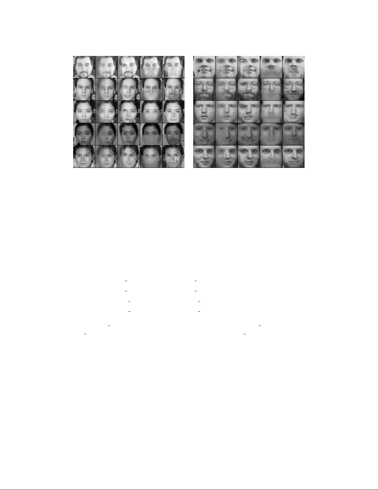
Journal of Machine Learning Research 18 (2017) 1-67 Submitted 12/15; Revised 12/16; Published 10/17 Hinge-Loss Mark o v Random Fields and Probabilistic Soft Logic Stephen H. Bac h bach@cs.st anford.edu Computer Scienc e Dep artment Stanfor d University Stanfor d, CA 94305, USA Matthias Bro ec heler ma tthias@da t ast ax.com DataStax Bert Huang bhuang@vt.edu Computer Scienc e Dep artment Vir ginia T e ch Blacksbur g, V A 24061, USA Lise Geto or getoor@soe.ucsc.edu Computer Scienc e Dep artment University of California, Santa Cruz Santa Cruz, CA 95064, USA Editor: Luc De Raedt Abstract A fundamen tal challenge in developing high-impact machine learning technologies is bal- ancing the need to mo del rich, structured domains with the abilit y to scale to big data. Man y important problem areas are b oth richly structured and large scale, from so cial and biological net w orks, to kno wledge graphs and the W eb, to images, video, and natural lan- guage. In this pap er, w e in tro duce t w o new formalisms for modeling structured data, and sho w that they can b oth capture ric h structure and scale to big data. The ﬁrst, hinge- loss Marko v random ﬁelds (HL-MRFs), is a new kind of probabilistic graphical model that generalizes diﬀeren t approac hes to conv ex inference. W e unite three approaches from the randomized algorithms, probabilistic graphical mo dels, and fuzzy logic communities, sho wing that all three lead to the same inference ob jectiv e. W e then deﬁne HL-MRFs b y generalizing this uniﬁed ob jective. The second new formalism, probabilistic soft logic (PSL), is a probabilistic programming language that makes HL-MRFs easy to deﬁne using a syntax based on ﬁrst-order logic. W e introduce an algorithm for inferring most-probable v ariable assignments (MAP inference) that is m uch more scalable than general-purp ose con vex optimization metho ds, b ecause it uses message passing to tak e adv an tage of sparse dep endency structures. W e then sho w ho w to learn the parameters of HL- MRFs. The learned HL-MRFs are as accurate as analogous discrete mo dels, but muc h more scalable. T ogether, these algorithms enable HL-MRFs and PSL to mo del rich, structured data at scales not previously p ossible. Keyw ords: Probabilistic graphical mo dels, statistical relational learning, structured prediction c  2017 Stephen H. Bach, Matthias Bro echeler, Bert Huang, and Lise Getoor. License: CC-BY 4.0, see https://creativecommons.org/licenses/by/4.0/ . Attribution requiremen ts are provided at http://jmlr.org/papers/v18/15- 631.html . Bach, Broecheler, Huang, and Getoor 1. In tro duction In man y problems in machine learning, the domains are rich and structured, with man y in terdep endent elements that are best mo deled jointly . Examples include so cial netw orks, biological net works, the W eb, natural language, computer vision, sensor netw orks, and so on. Mac hine learning subﬁelds suc h as statistical relational learning (Geto or and T ask ar, 2007), inductiv e logic programming (Muggleton and De Raedt, 1994), and structured prediction (Bakir et al., 2007) all seek to represent dependencies in data induced b y relational structure. With the ev er-increasing size of av ailable data, there is a gro wing need for mo dels that are highly scalable while still able to capture rich structure. In this paper, w e introduce hinge-loss Markov r andom ﬁelds (HL-MRFs), a new class of probabilistic graphical models designed to enable scalable mo deling of rich, structured data. HL-MRFs are analogous to discrete MRFs, which are undirected probabilistic graphical mo dels in whic h probabilit y mass is log-prop ortional to a w eigh ted sum of feature functions. Unlik e discrete MRFs, how ev er, HL-MRFs are deﬁned ov er con tin uous v ariables in the [0 , 1] unit interv al. T o mo del dep endencies among these contin uous v ariables, w e use linear and quadratic hinge functions, so that probability densit y is lost according to a weigh ted sum of hinge losses. As we will sho w, hinge-loss features capture man y common modeling patterns for structured data. When designing classes of models, there is generally a trade oﬀ b et ween scalabilit y and expressivit y: the more complex the t yp es and connectivit y structure of the dep endencies, the more computationally c hallenging inference and learning become. HL-MRFs address a crucial gap b et ween the tw o extremes. By using hinge-loss functions to model the de- p endencies among the v ariables, which admit highly scalable inference without restrictions on their connectivity structure, HL-MRFs can capture a wide range of useful relationships. One reason they are so expressiv e is that hinge-loss dep endencies are at the core of a n um b er of scalable techniques for mo deling b oth discrete and contin uous structured data. T o motiv ate HL-MRFs, w e unify three diﬀerent approaches for scalable inference in structured mo dels: (1) randomized algorithms for MAX SA T (Goemans and Williamson, 1994), (2) lo cal consistency relaxation (W ainwrigh t and Jordan, 2008) for discrete Marko v random ﬁelds deﬁned using Boolean logic, and (3) reasoning about contin uous information with fuzzy logic. W e sho w that all three approac hes lead to the same con v ex programming ob jectiv e. W e then deﬁne HL-MRFs by generalizing this uniﬁed inference ob jective as a w eighted sum of hinge-loss features and using them as the w eighted features of graphical mo dels. Since HL-MRFs generalize approac hes that reason ab out relational data with w eighted logical kno wledge bases, they retain the same high lev el of expressivit y . As w e sho w in Section 6.4, they are eﬀectiv e for mo deling b oth discrete and con tinuous data. W e also introduce pr ob abilistic soft lo gic (PSL), a new probabilistic programming lan- guage that mak es HL-MRFs easy to deﬁne and use for large, relational data sets. 1 This idea has b een explored for other classes of models, suc h as Marko v logic netw orks (Richard- son and Domingos, 2006) for discrete MRFs, relational dep endency netw orks (Neville and Jensen, 2007) for dep endency netw orks, and probabilistic relational mo dels (Geto or et al., 2002) for Bay esian net works. W e build on these previous approac hes, as well as the con- nection b etw een hinge-loss p otentials and logical clauses, to deﬁne PSL. In addition to 1. An op en source implementation, tutorials, and data sets are av ailable at http://psl.linqs.org . 2 Hinge-Loss Markov Random Fields and Probabilistic Soft Logic probabilistic rules, PSL pro vides syn tax that enables users to easily apply many common mo deling tec hniques, suc h as domain and range constraints, blo cking and canop y functions, and aggregate v ariables deﬁned ov er other random v ariables. Our next contribution is to introduce a num b er of inference and learning algorithms. First, we examine MAP inference, i.e., the problem of ﬁnding a most probable assignment to the unobserv ed random v ariables. MAP inference in HL-MRFs is alwa ys a con vex op- timization. Although any oﬀ-the-shelf optimization to olkit could b e used, such methods t ypically do not leverage the sparse dep endency structures common in graphical models. W e in troduce a consensus-optimization approach to MAP inference for HL-MRFs, showing ho w the problem can b e decomp osed using the alternating direction metho d of multipliers (ADMM) and ho w the resulting subproblems can b e solved analytically for hinge-loss poten- tials. Our approac h enables HL-MRFs to easily scale b eyond the capabilities of oﬀ-the-shelf optimization softw are or sampling-based inference in discrete MRFs. W e then sho w ho w to learn HL-MRFs from training data using a v ariet y of metho ds: structured p erceptron, maxim um pseudolikelihoo d, and large margin estimation. Since structured p erceptron and large margin estimation rely on inference as subroutines, and maxim um pseudolikelihoo d estimation is eﬃcient by design, all of these metho ds are highly scalable for HL-MRFs. W e ev aluate them on core relational learning and structured prediction tasks, suc h as collec- tiv e classiﬁcation and link prediction. W e sho w that HL-MRFs oﬀer predictiv e accuracy comparable to analogous discrete mo dels while scaling muc h b etter to large data sets. This pap er brings together and expands w ork on scalable models for structured data that can be either discrete, contin uous, or a mixture of both (Broecheler et al., 2010a; Bac h et al., 2012, 2013, 2015b). The eﬀectiv eness of HL-MRFs and PSL has b een demonstrated on many problems, including information extraction (Liu et al., 2016) and automatic knowledge base construction (Pujara et al., 2013), extracting and ev aluating natural-language arguments on the W eb (Samadi et al., 2016), high-lev el computer vision (London et al., 2013), drug disco very (F akhraei et al., 2014) and predicting drug-drug interactions (Sridhar et al., 2016), natural language semantics (Beltagy et al., 2014; Sridhar et al., 2015; Deng and Wieb e, 2015; Ebrahimi et al., 2016), automobile-traﬃc modeling (Chen et al., 2014), recommender systems (Kouki et al., 2015), information retriev al (Alsh uk aili et al., 2016), and predicting attributes (Li et al., 2014) and trust (Huang et al., 2013; W est et al., 2014) in so cial netw orks. The abilit y to easily incorporate latent v ariables into HL-MRFs and PSL (Bach et al., 2015a) has enabled further applications, including mo deling latent topics in text (F oulds et al., 2015), and predicting studen t outcomes in massiv e open online courses (MOOCs) (Ramesh et al., 2014, 2015). Researchers ha ve also studied ho w to mak e HL-MRFs and PSL ev en more scalable by dev eloping distributed implementations (Miao et al., 2013; Magliacane et al., 2015). That they are already b eing widely applied indicates HL-MRFs and PSL address an op en need in the machine learning comm unity . The pap er is organized as follo ws. In Section 2, w e ﬁrst consider mo dels for structured prediction that are deﬁned using logical clauses. W e unify three diﬀerent approac hes to scalable inference in suc h mo dels, sho wing that they all optimize the same con vex ob jec- tiv e. W e then generalize this ob jectiv e in Section 3 to deﬁne HL-MRFs. In Section 4, w e in tro duce PSL, specifying the language and giving many examples of common usage. Next w e in tro duce a scalable message-passing algorithm for MAP inference in Section 5 and a 3 Bach, Broecheler, Huang, and Getoor n umber of learning algorithms in Section 6, ev aluating them on a range of tasks. Finally , in Section 7, we discuss related work. 2. Unifying Con v ex Inference for Logic-Based Graphical Models In man y structured domains, prop ositional and ﬁrst-order logics are useful to ols for describ- ing the in tricate dependencies that connect the unkno wn v ariables. How ev er, these domains are usually noisy; dep endencies among the v ariables do not alw ays hold. T o address this, logical seman tics can b e incorp orated in to probability distributions to create mo dels that capture both the structure and the uncertain ty in mac hine learning tasks. One common w ay to do this is to use logic to deﬁne feature functions in a probabilistic model. W e focus on Mark ov random ﬁelds (MRFs), a p opular class of probabilistic graphical mo dels. Infor- mally , an MRF is a distribution that assigns probabilit y mass using a scoring function that is a weigh ted com bination of feature functions called p oten tials. W e will use logical clauses to deﬁne these p otentials. W e ﬁrst deﬁne MRFs more formally to introduce necessary notation: Deﬁnition 1 L et x = ( x 1 , . . . , x n ) b e a ve ctor of r andom variables and let φ = ( φ 1 , . . . , φ m ) b e a ve ctor of p otentials wher e e ach p otential φ j ( x ) assigns c onﬁgur ations of the variables a r e al-value d sc or e. Also, let w = ( w 1 , . . . , w m ) b e a ve ctor of r e al-value d weights. Then, a Mark o v random ﬁeld is a pr ob ability distribution of the form P ( x ) ∝ exp  w > φ ( x )  . (1) In an MRF, the p oten tials should capture ho w the domain behav es, assigning higher scores to more probable conﬁgurations of the v ariables. If a mo deler do es not kno w how the domain b eha v es, the p oten tials should capture ho w it migh t b eha ve, so that a learning algorithm can ﬁnd w eigh ts that lead to accurate predictions. Logic provides an excellent formalism for deﬁning such p oten tials in structured and relational domains. W e no w introduce some notation to make this logic-based approac h more formal. Con- sider a set of logical clauses C = { C 1 , . . . , C m } , i.e., a kno wledge base, where each clause C j ∈ C is a disjunction of literals and each literal is a v ariable x or its negation ¬ x drawn from the v ariables x such that each v ariable x i ∈ x app ears at most once in C j . Let I + j (resp. I − j ) ⊂ { 1 , . . . , n } be the set of indices of the v ariables that are not negated (resp. negated) in C j . Then C j can b e written as    _ i ∈ I + j x i    _    _ i ∈ I − j ¬ x i    . (2) Logical clauses of this form are expressive b ecause they can b e viewed equiv alen tly as implications from conditions to consequences: ^ i ∈ I − j x i = ⇒ _ i ∈ I + j x i . (3) This “if-then” reasoning is intui tive and can describ e man y dependencies in structured data. 4 Hinge-Loss Markov Random Fields and Probabilistic Soft Logic Assuming w e hav e a logical kno wledge base C describing a structured domain, we can em b ed it in an MRF by deﬁning eac h potential φ j using a corresponding clause C j . If an assignmen t to the v ariables x satisﬁes C j , then we let φ j ( x ) equal 1, and we let it equal 0 otherwise. F or our subsequen t analysis we assume w j ≥ 0 ( ∀ j = 1 , . . . , m ). The resulting MRF preserves the structured dep endencies described in C but enables muc h more ﬂexible mo deling. Clauses no longer m ust alwa ys hold, and the model can express uncertaint y o ver diﬀerent p ossible worlds. The w eights express how strongly the mo del expects eac h corresp onding clause to hold; the higher the weigh t, the more probable that it is true according to the mo del. This notion of embedding weigh ted, logical knowledge bases in MRFs is an app ealing one. F or example, Marko v logic (Richardson and Domingos, 2006) is a popular formalism that induces MRFs from weigh ted ﬁrst-order knowledge bases. Given a data set, the ﬁrst- order clauses are grounded using the constants in the data to create the set of prop ositional clauses C . Each prop ositional clause has the weigh t of the ﬁrst-order clause from which it w as grounded. In this w a y , a w eighted, ﬁrst-order knowledge base can compactly sp ecify an entire family of MRFs for a structured mac hine-learning task. Although we now ha ve a metho d for easily deﬁning rich, structured mo dels for a wide range of problems, there is a new c hallenge: ﬁnding a most probable assignmen t to the v ariables, i.e., MAP inference, is NP-hard (Shimon y, 1994; Garey et al., 1976). This means that (unless P=NP) our only hop e for p erforming tractable inference is to p erform it ap- pro ximately . Observ e that MAP inference for an MRF deﬁned by C is the integer linear program arg max x ∈{ 0 , 1 } n P ( x ) ≡ arg max x ∈{ 0 , 1 } n w > φ ( x ) ≡ arg max x ∈{ 0 , 1 } n X C j ∈ C w j min      X i ∈ I + j x i + X i ∈ I − j (1 − x i ) , 1      . (4) While this program is in tractable, it do es admit conv ex programming relaxations. In this section, w e show how con v ex programming can b e used to p erform tractable inference in MRFs deﬁned b y w eighted kno wledge bases. W e ﬁrst discuss in Section 2.1 an approac h developed by Go emans and Williamson (1994) that views MAP inference as an instance of the classic MAX SA T problem and relaxes it to a conv ex program from that p ersp ectiv e. This approach has the adv antage of pro viding strong guaran tees on the quality of the discrete solutions it obtains. Ho wev er, it has the disadv an tage that general-purp ose con vex programming to olkits do not scale w ell to relaxed MAP inference for large graphical mo dels (Y ano ver et al., 2006). In Section 2.2 w e then discuss a seemingly distinct approach, lo cal consistency relaxation, with complementary adv antages and disadv an tages: it oﬀers highly scalable message-passing algorithms but comes with no qualit y guaran tees. W e then unite these approaches b y pro ving that they solv e equiv alen t optimization problems with iden tical solutions. Then, in Section 2.3, w e show that the uniﬁed inference ob jectiv e is also equiv alen t to exact MAP inference if the kno wledge base C is interpreted using Luk asiewicz logic, an inﬁnite-v alued logic for reasoning ab out naturally contin uous quan tities such as similarit y , v ague or fuzzy concepts, and real-v alued data. 5 Bach, Broecheler, Huang, and Getoor That these three interpretations all lead to the same inference ob jectiv e—whether rea- soning ab out discrete or con tin uous information—is useful. T o the b est of our kno wledge, w e are the ﬁrst to show their equiv alence. This equiv alence indicates that the same mo del- ing formalism, inference algorithms, and learning algorithms can b e used to reason scalably and accurately about b oth discrete and contin uous information in structured domains. W e generalize the uniﬁed inference ob jectiv e in Section 3.1 to deﬁne hinge-loss MRFs, and in the rest of the paper w e develop a probabilistic programming language and algorithms that realize the goal of a scalable and accurate framework for structured data, b oth discrete and con tinuous. 2.1 MAX SA T Relaxation One approach to appro ximating ob jective (4) is to use relaxation techniques developed in the randomized algorithms communit y for the MAX SA T problem. F ormally , the MAX SA T problem is to ﬁnd a Bo olean assignmen t to a set of v ariables that maximizes the total w eight of satisﬁed clauses in a kno wledge base comp osed of disjunctive clauses annotated with nonnegative weigh ts. In other words, ob jectiv e (4) is an instance of MAX SA T. Randomized approximation algorithms can b e constructed for MAX SA T by indep enden tly rounding each Boolean v ariable x i to true with probability p i . Then, the expected weigh ted satisfaction ˆ w j of a clause C j is ˆ w j = w j    1 − Y i ∈ I + j (1 − p i ) Y i ∈ I − j p i    , (5) also known as a (w eighted) noisy-or function, and the exp ected total score ˆ W is ˆ W = X C j ∈ C w j    1 − Y i ∈ I + j (1 − p i ) Y i ∈ I − j p i    . (6) Optimizing ˆ W with resp ect to the rounding probabilities w ould giv e the exact MAX SA T so- lution, so this randomized approac h has not made the problem any easier y et, but Go emans and Williamson (1994) show ed how to b ound ˆ W b elow with a tractable linear program. T o approximately optimize ˆ W , asso ciate with eac h Boolean v ariable x i a corresponding con tinuous v ariable ˆ y i with domain [0 , 1]. Then let ˆ y ? b e the optim um of the linear program arg max ˆ y ∈ [0 , 1] n X C j ∈ C w j min      X i ∈ I + j ˆ y i + X i ∈ I − j (1 − ˆ y i ) , 1      . (7) Observ e that ob jectiv es (4) and (7) are of the same form, except that the v ariables are relaxed to the unit h yp ercube in ob jectiv e (7). Go emans and Williamson (1994) pro ved that if p i is set to ˆ y ? i for all i , then ˆ W ≥ . 632 Z ? , where Z ? is the optimal total weigh t for the MAX SA T problem. If each p i is set using an y function in a sp ecial class, then this 6 Hinge-Loss Markov Random Fields and Probabilistic Soft Logic lo wer bound impro ves to a .75 approximation. One simple example of such a function is p i = 1 2 ˆ y ? i + 1 4 . (8) In this w ay , ob jectiv e (7) leads to an exp ected .75 appro ximation of the MAX SA T solution. The follo wing metho d of conditional probabilities (Alon and Spencer, 2008) can ﬁnd a single Bo olean assignment that achiev es at least the exp ected score from a set of rounding probabilities, and therefore at least .75 of the MAX SA T solution when ob jectiv e (7) and function (8) are used to obtain them. Each v ariable x i is greedily set to the v alue that maximizes the expected w eight ov er the unassigned v ariables, conditioned on either p ossible v alue of x i and the previously assigned v ariables. This greedy maximization can b e applied quic kly because, in many models, v ariables only participate in a small fraction of the clauses, making the change in exp ectation quic k to compute for eac h v ariable. Sp eciﬁcally , referring to the deﬁnition of ˆ W (6), the assignmen t to x i only needs to maximize o ver the clauses C j in which x i participates, i.e., i ∈ I + j ∪ I − j , which is usually a small set. This approximation is p ow erful b ecause it is a tractable linear program that comes with strong guaran tees on solution quality . Ho w ever, even though it is tractable, general- purp ose con vex optimization to olkits do not scale w ell to large MAP problems. In the follo wing subsection, we unify this approximation with a complementary one dev elop ed in the probabilistic graphical mo dels communit y . 2.2 Lo cal Consistency Relaxation Another approach to approximating ob jectiv e (4) is to apply a relaxation developed for Mark ov random ﬁelds called lo cal consistency relaxation (W ainwrigh t and Jordan, 2008). This approac h starts by viewing MAP inference as an equiv alent optimization o ver marginal probabilities. 2 F or eac h φ j ∈ φ , let θ j b e a marginal distribution o ver join t assignmen ts x j . F or example, θ j ( x j ) is the probability that the subset of v ariables associated with p otential φ j is in a particular joint state x j . Also, let x j ( i ) denote the setting of the v ariable with index i in the state x j . With this v ariational formulation, inference can b e relaxed to an optimization o ver the ﬁrst-or der lo c al p olytop e L . Let µ = ( µ 1 , . . . , µ n ) b e a vector of probability distributions, where µ i ( k ) is the marginal probability that x i is in state k . The ﬁrst-order local p olytop e is L ,        ( θ , µ ) ≥ 0         P x j | x j ( i )= k θ j ( x j ) = µ i ( k ) ∀ i, j, k P x j θ j ( x j ) = 1 ∀ j P K i − 1 k =0 µ i ( k ) = 1 ∀ i        , (9) whic h constrains eac h marginal distribution θ j o ver joint states x j to be consisten t only with the marginal distributions µ o v er individual v ariables that participate in the potential φ j . MAP inference can then be appro ximated with the ﬁrst-or der lo c al c onsistency r elax- ation : arg max ( θ , µ ) ∈ L m X j =1 w j X x j θ j ( x j ) φ j ( x j ) , (10) 2. This treatment is for discrete MRFs. W e hav e omitted a discussion of contin uous MRFs for conciseness. 7 Bach, Broecheler, Huang, and Getoor whic h is an upp er b ound on the true MAP ob jectiv e. Much work has focused on solving the ﬁrst-order lo cal consistency relaxation for large-scale MRFs, which we discuss further in Section 7. These algorithms are app ealing because they are w ell-suited to the sparse dep endency structures common in MRFs, so they can scale to large problems. Ho wev er, in general, the solutions can b e fractional, and there are no guarantees on the approximation qualit y of a tractable discretization of these fractional solutions. W e sho w that for MRFs with p otentials deﬁned by C and nonnegative weigh ts, local consistency relaxation is equiv alen t to MAX SA T relaxation. Theorem 2 F or an MRF with p otentials c orr esp onding to disjunctive lo gic al clauses and asso ciate d nonne gative weights, the ﬁrst-or der lo c al c onsistency r elaxation of MAP infer enc e is e quivalent to the MAX SA T r elaxation of Go emans and Wil liamson (1994). Sp e ciﬁc al ly, any p artial optimum µ ? of obje ctive (10) is an optimum ˆ y ? of obje ctive (7), and vic e versa. W e pro v e Theorem 2 in App endix A. Our pro of analyzes the lo cal consistency relaxation to deriv e an equiv alent, more compact optimization o ver only the v ariable pseudomarginals µ that is iden tical to the MAX SA T relaxation. Theorem 2 is signiﬁcan t b ecause it sho ws that the rounding guaran tees of MAX SA T relaxation also apply to lo cal consistency relaxation, and the scalable message-passing algorithms dev elop ed for lo cal consistency relaxation also apply to MAX SA T relaxation. 2.3 Luk asiewicz Logic The previous t wo subsections sho w ed that the same conv ex program can approximate MAP inference in discrete, logic-based mo dels, whether view ed from the p ersp ectiv e of randomized algorithms or v ariational metho ds. In this subsection, we show that this conv ex program can also b e used to reason ab out naturally con tin uous information, suc h as similarit y , v ague or fuzzy concepts, and real-v alued data. Instead of in terpreting the clauses C using Boolean logic, we can interpret them using Luk asiewicz logic (Klir and Y uan, 1995), which extends Bo olean logic to inﬁnite-v alued logic in whic h the propositions x can tak e truth v alues in the con tinuous interv al [0 , 1]. Extending truth v alues to a con tin uous domain enables them to represen t concepts that are v ague, in the sense that they are often neither completely true nor completely false. F or example, the prop ositions that a sensor v alue is high, t wo entities are similar, or a protein is highly expressed can all be captured in a more nuanced manner in Luk asiewicz logic. W e can also use the now con tinuous v alued x to represent quantities that are naturally con tinuous (scaled to [0,1]), suc h as actual sensor v alues, similarit y scores, and protein expression lev els. The ability to reason about con tinuous v alues is v aluable, as man y imp ortant applications are not entirely discrete. The extension to con tinuous v alues requires a corresp onding extended in terpretation of the logical op erators ∧ (conjunction), ∨ (disjunction), and ¬ (negation). The Luk asiewicz t-norm and t-co-norm are ∧ and ∨ op erators that corresp ond to the Bo olean logic operators for integer inputs (along with the negation op erator ¬ ): x 1 ∧ x 2 = max { x 1 + x 2 − 1 , 0 } (11) x 1 ∨ x 2 = min { x 1 + x 2 , 1 } (12) ¬ x = 1 − x . (13) 8 Hinge-Loss Markov Random Fields and Probabilistic Soft Logic The analogous MAX SA T problem for Luk asiewicz logic is therefore arg max x ∈ [0 , 1] n X C j ∈ C w j min      X i ∈ I + j x i + X i ∈ I − j (1 − x i ) , 1      , (14) whic h is iden tical in form to the relaxed MAX SA T ob jectiv e (7). Therefore, if an MRF is deﬁned o ver contin uous v ariables with domain [0 , 1] n and the logical knowledge base C deﬁning the p otentials is interpreted using Luk asiewicz logic, then exact MAP inference is iden tical to ﬁnding the optim um using the uniﬁed, relaxed inference ob jective deriv ed for Bo olean logic in the previous tw o subsections. This result shows the equiv alence of all three approaches: MAX SA T relaxation, lo cal consistency relaxation, and MAX SA T using Luk asiewicz logic. 3. Hinge-Loss Mark o v Random Fields W e hav e sho wn that a sp eciﬁc family of con v ex programs can b e used to reason scalably and accurately about b oth discrete and contin uous information. In this section, w e generalize this family to deﬁne hinge-loss Markov r andom ﬁelds (HL-MRFs), a new kind of probabilis- tic graphical mo del. HL-MRFs retain the con vexit y and expressivity of conv ex programs discussed in Section 2, and additionally supp ort an ev en richer space of dep endencies. T o begin, we deﬁne HL-MRFs as density functions o v er contin uous v ariables y = ( y 1 , . . . , y n ) with join t domain [0 , 1] n . These v ariables ha v e diﬀeren t p ossible in terpreta- tions dep ending on the application. Since w e are generalizing the interpretations explored in Section 2, HL-MRF MAP states can b e view ed as rounding probabilities or pseudo- marginals, or they can represen t naturally con tinuous information. More generally , they can b e view ed simply as degrees of belief, conﬁdences, or rankings of p ossible states; and they can describ e discrete, con tinuous, or mixed domains. The application domain typi- cally determines which in terpretation is most appropriate. The formalisms and algorithms describ ed in the rest of this pap er are general with resp ect to such in terpretations. 3.1 Generalized Inference Ob jectiv e T o deﬁne HL-MRFs, w e will ﬁrst generalize the uniﬁed inference ob jectiv e of Section 2 in sev eral wa ys, which w e ﬁrst restate in terms of the HL-MRF v ariables y : arg max y ∈ [0 , 1] n X C j ∈ C w j min      X i ∈ I + j y i + X i ∈ I − j (1 − y i ) , 1      . (15) F or no w, w e are still assuming that the ob jectiv e terms are deﬁned using a weigh ted knowl- edge base C , but w e will quickly drop this requiremen t. T o do so, we examine one term in isolation. Observe that the maxim um v alue of any un w eighted term is 1, which is ac hiev ed when a linear function of the v ariables is at least 1. W e sa y that the term is satisﬁe d when- ev er this o ccurs. When a term is unsatisﬁed, w e can refer to its distanc e to satisfaction , whic h is how far it is from achieving its maxim um v alue. Also observ e that we can rewrite 9 Bach, Broecheler, Huang, and Getoor the optimization explicitly in terms of distances to satisfaction: arg min y ∈ [0 , 1] n X C j ∈ C w j max      1 − X i ∈ I + j y i − X i ∈ I − j (1 − y i ) , 0      , (16) so that the ob jective is equiv alen tly to minimize the total w eigh ted distance to satisfaction. Eac h unw eigh ted ob jectiv e term now measures ho w far the linear constraint 1 − X i ∈ I + j y i − X i ∈ I − j (1 − y i ) ≤ 0 (17) is from b eing satisﬁed. 3.1.1 Relaxed Linear Constraints With this view of each term as a relaxed linear constrain t, w e can easily generalize them to arbitrary linear constraints. W e no longer require that the inference ob jective b e deﬁned using only logical clauses, and instead eac h term can b e deﬁned using an y function ` j ( y ) that is linear in y . These functions can capture more general dep endencies, such as b eliefs ab out the range of v alues a v ariable can tak e and arithmetic relationships among v ariables. The new inference ob jective is arg min y ∈ [0 , 1] n m X j =1 w j max { ` j ( y ) , 0 } . (18) In this form, each term represe n ts the distance to satisfaction of a linear constrain t ` j ( y ) ≤ 0. That constrain t could b e deﬁned using logical clauses as discussed ab ov e, or it could b e deﬁned using other kno wledge ab out the domain. The weigh t w j indicates ho w imp ortant it is to satisfy a constraint relativ e to others by scaling the distance to satisfaction. The higher the weigh t, the more distance to satisfaction is p enalized. Additionally , tw o relaxed inequalit y constrain ts, ` j ( y ) ≤ 0 and − ` j ( y ) ≤ 0, can b e combined to represent a relaxed equalit y constraint ` j ( y ) = 0. 3.1.2 Hard Linear Constraints No w that our inference ob jectiv e admits arbitrary relaxed linear constrain ts, it is natural to also allow hard constraints that m ust b e satisﬁed at all times. Hard constrain ts are imp ortan t mo deling to ols. They enable groups of v ariables to represen t m utually exclusive p ossibilities, suc h as a multinomial or categorical v ariable, and functional or partial func- tional relationships. Hard constraints can also represen t background knowledge ab out the domain, restricting the domain to regions that are feasible in the real world. Additionally , they can encode more complex model components suc h as deﬁning a random v ariable as an aggregate ov er other unobserv ed v ariables, whic h we discuss further in Section 4.3.5. W e can think of including hard constrain ts as allowing a weigh t w j to take an inﬁnite v alue. Again, t wo inequality constrain ts can b e com bined to represent an equalit y con- strain t. Ho wev er, when w e introduce an inference algorithm for HL-MRFs in Section 5, it 10 Hinge-Loss Markov Random Fields and Probabilistic Soft Logic will b e useful to treat hard constrain ts separately from relaxed ones, and further, treat hard inequalit y constrain ts separately from hard equality constraints. Therefore, in the deﬁnition of HL-MRFs, we will deﬁne these three comp onents separately . 3.1.3 Generalized Hinge-Loss Functions The ob jectiv e terms measuring each constrain t’s distance to satisfaction are hinge losses. There is a ﬂat region, on which the distance to satisfaction is 0, and an angled region, on whic h the distance to satisfaction gro ws linearly a w ay from the h yp erplane ` j ( y ) = 0. This loss function is useful—as w e discuss in the previous section, it is a b ound on the exp ected loss in the discrete setting, among other things—but it is not appropriate for all mo deling situations. A piecewise-linear loss function makes MAP inference “winner tak e all,” in the sense that it is preferable to fully satisfy the most highly w eighted ob jectiv e terms completely b efore reducing the distance to satisfaction of terms with lo w er w eights. F or example, consider the following optimization problem: arg min y 1 ∈ [0 , 1] w 1 max { y 1 , 0 } + w 2 max { 1 − y 1 , 0 } . (19) If w 1 > w 2 ≥ 0, then the optimizer is y 1 = 0 because the term that prefers y 1 = 0 o v errules the term that prefers y 1 = 1. The result does not indicate an y am biguit y or uncertain t y , but if the t wo ob jectiv e terms are p oten tials in a probabilistic mo del, it is sometimes preferable that the result reﬂect the conﬂicting preferences. W e can change the inference problem so that it smo othly trades oﬀ satisfying c onﬂicting ob jective terms by squaring the hinge losses. Observe that in the mo diﬁed problem arg m in y 1 ∈ [0 , 1] w 1 (max { y 1 , 0 } ) 2 + w 2 (max { 1 − y 1 , 0 } ) 2 (20) the optimizer is now y 1 = w 2 w 1 + w 2 , reﬂecting the relative inﬂuence of the tw o loss functions. Another adv antage of squared hinge-loss functions is that they can behav e more in tu- itiv ely in the presence of hard constrain ts. Consider the problem arg m in ( y 1 ,y 2 ) ∈ [0 , 1] 2 max { 0 . 9 − y 1 , 0 } + max { 0 . 6 − y 2 , 0 } suc h that y 1 + y 2 ≤ 1 . (21) The ﬁrst term prefers y 1 ≥ 0 . 9, the second term prefers y 2 ≥ 0 . 6, and the constrain t requires that y 1 and y 2 are m utually exclusiv e. Such problems are very common and arise when conﬂicting evidence of diﬀerent strengths supp ort tw o m utually exclusiv e possibilities. The evidence v alues 0.9 and 0.6 could come from man y sources, including base mo dels trained to mak e independent predictions on individual random v ariables, domain-specialized similarit y functions, or sensor readings. F or this problem, an y solution y 1 ∈ [0 . 4 , 0 . 9] and y 2 = 1 − y 1 is an optimizer. This solution set includes coun terintuitiv e optimizers like y 1 = 0 . 4 and y 2 = 0 . 6, even though the evidence supp orting y 1 is stronger. Again, squared hinge losses 11 Bach, Broecheler, Huang, and Getoor ensure the optimizers b etter reﬂect the relative strength of evidence. F or the problem arg min ( y 1 ,y 2 ) ∈ [0 , 1] 2 (max { 0 . 9 − y 1 , 0 } ) 2 + (max { 0 . 6 − y 2 , 0 } ) 2 suc h that y 1 + y 2 ≤ 1 , (22) the only optimizer is y 1 = 0 . 65 and y 2 = 0 . 35, which is a more informativ e solution. W e therefore complete our generalized inference ob jective b y allowing either hinge-loss or squared hinge-loss functions. Users of HL-MRFs ha ve the c hoice of either one for each p oten tial, dep ending on whic h is appropriate for their task. 3.2 Deﬁnition W e can now formally state the full deﬁnition of HL-MRFs. They are deﬁned so that a MAP state is a solution to the generalized inference ob jective prop osed in the previous subsection. W e state the deﬁnition in a conditional form for later con venience, but this deﬁnition is fully general since the vector of conditioning v ariables ma y b e empt y . Deﬁnition 3 L et y = ( y 1 , . . . , y n ) b e a ve ctor of n variables and x = ( x 1 , . . . , x n 0 ) a ve ctor of n 0 variables with joint domain D = [0 , 1] n + n 0 . L et φ = ( φ 1 , . . . , φ m ) b e a ve ctor of m c ontinuous p otentials of the form φ j ( y , x ) = (max { ` j ( y , x ) , 0 } ) p j (23) wher e ` j is a line ar function of y and x and p j ∈ { 1 , 2 } . L et c = ( c 1 , . . . , c r ) b e a ve ctor of r line ar c onstr aint functions asso ciate d with index sets denoting e quality c onstr aints E and ine quality c onstr aints I , which deﬁne the fe asible set ˜ D =  ( y , x ) ∈ D     c k ( y , x ) = 0 , ∀ k ∈ E c k ( y , x ) ≤ 0 , ∀ k ∈ I  . (24) F or ( y , x ) ∈ D , given a ve ctor of m nonne gative fr e e p ar ameters, i.e., weights, w = ( w 1 , . . . , w m ) , a constrained hinge-loss energy function f w is deﬁne d as f w ( y , x ) = m X j =1 w j φ j ( y , x ) . (25) W e now deﬁne HL-MRFs by placing a probability densit y o ver the inputs to a con- strained hinge-loss energy function. Note that we negate the hinge-loss energy function so that states with lo wer energy are more probable, in con trast with Deﬁnition 1. This c hange is made for later notational conv enience. Deﬁnition 4 A hinge-loss Mark ov random ﬁeld P over r andom variables y and c on- ditione d on r andom variables x is a pr ob ability density deﬁne d as fol lows: if ( y , x ) / ∈ ˜ D , then P ( y | x ) = 0 ; if ( y , x ) ∈ ˜ D , then P ( y | x ) = 1 Z ( w , x ) exp ( − f w ( y , x )) (26) 12 Hinge-Loss Markov Random Fields and Probabilistic Soft Logic wher e Z ( w , x ) = Z y | ( y , x ) ∈ ˜ D exp ( − f w ( y , x )) d y . (27) In the rest of this paper, we will explore ho w to use HL-MRFs to solv e a wide range of structured mac hine learning problems. W e ﬁrst in tro duce a probabilistic programming language that makes HL-MRFs easy to deﬁne for large, rich domains. 4. Probabilistic Soft Logic In this section we introduce a general-purpose probabilistic programming language, pr ob- abilistic soft lo gic (PSL). PSL allows HL-MRFs to b e easily applied to a broad range of structured mac hine learning problems b y deﬁning templates for potentials and constrain ts. In mo dels for structured data, there are v ery often rep eated patterns of probabilistic de- p endencies. A few of the many examples include the strength of ties betw een similar p eople in so cial net works, the preference for triadic closure when predicting transitive relation- ships, and the “exactly one active” constrain ts on functional relationships. Often, to make graphical models b oth easy to deﬁne and able to generalize across diﬀeren t data sets, these rep eated dep endencies are deﬁned using templates. Eac h template deﬁnes an abstract de- p endency , such as the form of a p otential function or constraint, along with any necessary parameters, such as the weigh t of the p oten tial, each of which has a single v alue across all dep endencies deﬁned by that template. Given input data, an undirected graphical mo del is constructed from a set of templates by ﬁrst iden tifying the random v ariables in the data and then “grounding out” eac h template b y introducing a p oten tial or constrain t into the graphical mo del for each subset of random v ariables to which the template applies. A PSL program is written in a declarative, ﬁrst-order syn tax and deﬁnes a class of HL-MRFs that are parameterized by the input data. PSL provides a natural interface to represen t hinge-loss potential templates using tw o t yp es of rules: logical rules and arithmetic rules. Logical rules are based on the mapping from logical clauses to hinge-loss p otentials in tro duced in Section 2. Arithmetic rules provide additional syn tax for deﬁning an even wider range of hinge-loss p oten tials and hard constraints. 4.1 Deﬁnition In this subsection we deﬁne PSL. Our deﬁnition cov ers the essen tial functionalit y that should b e supp orted by all implementations, but man y extensions are p ossible. The PSL syn tax we describ e can capture a wide range of HL-MRFs, but new settings and scenarios could motiv ate the developmen t of additional syntax to make the construction of diﬀerent kinds of HL-MRFs more con venien t. 4.1.1 Preliminaries W e b egin with a high-level deﬁnition of PSL programs. Deﬁnition 5 A PSL program is a set of rules, e ach of which is a template for hinge-loss p otentials or har d line ar c onstr aints. When gr ounde d over a b ase of gr ound atoms, a PSL pr o gr am induc es a HL-MRF c onditione d on any sp e ciﬁe d observations. 13 Bach, Broecheler, Huang, and Getoor In the PSL syn tax, man y comp onen ts are named using identiﬁers , whic h are strings that b egin with a letter (from the set { A , . . . , Z , a , . . . , z } ), follow ed b y zero or more letters, n umeric digits, or underscores. PSL programs are grounded out o v er data, so the universe ov er which to ground must b e deﬁned. Deﬁnition 6 A constant is a string that denotes an element in the universe over which a PSL pr o gr am is gr ounde d. Constan ts are the elements in a univ erse of discourse. They can b e en tities or attributes. F or example, the constant "person1" can denote a p erson, the constan t "Adam" can denote a p erson’s name, and the constant "30" can denote a p erson’s age. In PSL programs, constan ts are written as strings in double or single quotes. Constants use backslashes as escap e c haracters, so they can be used to enco de quotes within constan ts. It is assumed that constan ts are unam biguous, i.e., diﬀeren t constants refer to diﬀerent en tities and attributes. 3 Groups of constants can b e represen ted using v ariables. Deﬁnition 7 A v ariable is an identiﬁer for which c onstants c an b e substitute d. V ariables and constan ts are the argumen ts to logical predicates. T ogether, they are generi- cally referred to as terms. Deﬁnition 8 A term is either a c onstant or a variable. T erms are connected by relationships called predicates. Deﬁnition 9 A predicate is a r elation deﬁne d by a unique identiﬁer and a p ositive inte ger c al le d its arity, which denotes the numb er of terms it ac c epts as ar guments. Every pr e dic ate in a PSL pr o gr am must have a unique identiﬁer as its name. W e refer to a predicate using its identiﬁer and arit y app ended with a slash. F or example, the predicate Friends/2 is a binary predicate, i.e., taking tw o argumen ts, which represents whether tw o constants are friends. As another example, the predicate Name/2 can relate a p erson to the string that is that p erson’s name. As a third example, the predicate EnrolledInClass/3 can relate t wo en tities, a student and professor, with an additional attribute, the sub ject of the class. Predicates and terms are com bined to create atoms. Deﬁnition 10 An atom is a pr e dic ate c ombine d with a se quenc e of terms of length e qual to the pr e dic ate’s arity. This se quenc e is c al le d the atom’s ar guments. A n atom with only c onstants for ar guments is c al le d a gr ound atom. Ground atoms are the basic units of reasoning in PSL. Each represents an unkno wn or observ ation of interest and can tak e an y v alue in [0 , 1]. F or example, the ground atom Friends("person1", "person2") represen ts whether "person1" and "person2" are friends. A toms that are not ground are placeholders for sets of ground atoms. F or example, the atom Friends(X, Y) stands for all ground atoms that can be obtained by substituting constan ts for v ariables X and Y . 3. Note that am biguous references to underlying en tities can be mo deled b y using diﬀerent constan ts for diﬀeren t references and representing whether they refer to the same underlying entit y as a predicate. 14 Hinge-Loss Markov Random Fields and Probabilistic Soft Logic 4.1.2 Inputs As we ha ve already stated, PSL deﬁnes templates for hinge-loss p otentials and hard linear constrain ts that are grounded out o v er a data set to induce a HL-MRF. W e now describ e ho w that data set is represen ted and pro vided as the inputs to a PSL program. The ﬁrst inputs are tw o sets of predicates: a set C of close d predicates, the atoms of which are completely observ ed, and a set O of op en predicates, the atoms of which ma y be unobserved. The third input is the b ase A , whic h is the set of all ground atoms under consideration. All atoms in A must ha v e a predicate in either C or O . These are the atoms that can b e substituted into the rules and constrain ts of a PSL program, and each will later be asso ciated with a HL- MRF random v ariable with domain [0 , 1]. The ﬁnal input is a function O : A → [0 , 1] ∪ {∅} that maps the ground atoms in the base to either an observ ed v alue in [0 , 1] or a sym b ol ∅ indicating that it is unobserv ed. The function O is only v alid if all atoms with a predicate in C are mapped to a [0 , 1] v alue. Note that this deﬁnition makes the sets C and O redundan t in a sense, since they can b e derived from A and O , but it will b e conv enien t later to hav e C and O explicitly deﬁned. Ultimately , the method for specifying PSL’s inputs is implemen tation-sp eciﬁc, since diﬀeren t c hoices make it more or less con venien t for diﬀeren t scenarios. In this paper, w e will assume that C , O , A , and O exist, and we remain agnostic ab out ho w they were sp eciﬁed. How ever, to mak e this asp ect of using PSL more concrete, w e will describ e one p ossible metho d for deﬁning them here. Our example metho d for sp ecifying PSL’s inputs is text-based. The ﬁrst section of the text input is a deﬁnition of the constan ts in the universe, which are group ed in to types. An example universe deﬁnition follo ws. Person = { "alexis", "bob", "claudia", "david" } Professor = { "alexis", "bob" } Student = { "claudia", "david" } Subject = { "computer science", "statistics" } This univ erse includes six constan ts, four with tw o t yp es ( "alexis" , "bob" , "claudia" , and "david" ) and tw o with one t yp e ( "computer science" and "statistics" ). The next section of input is the deﬁnition of predicates. Each predicate includes the t yp es of constants it tak es as argumen ts and whether it is closed. F or example, we can deﬁne predicates for an advisor-studen t relationship prediction task as follo ws: Advises(Professor, Student) Department(Person, Subject) (closed) EnrolledInClass(Student, Subject, Professor) (closed) In this case, there is one op en predicate ( Advises ) and t wo closed predicates ( Department and EnrolledInClass ). 15 Bach, Broecheler, Huang, and Getoor The ﬁnal section of input is an y associated observ ations. They can b e sp eciﬁed in a list, for example: Advises("alexis", "david") = 1 Department("alexis", "computer science") = 1 Department("bob", "computer science") = 1 Department("claudia", "statistics") = 1 Department("david", "statistics") = 1 In addition, v alues for atoms with the EnrolledInClass predicate could also b e sp eciﬁed. If a ground atom do es not hav e a sp eciﬁed v alue, it will hav e a default observed v alue of 0 if its predicate is closed or remain unobserved if its predicate is op en. W e no w describ e how this text input is pro cessed into the formal inputs C , O , A , and O . First, each predicate is added to either C or O based on whether it is annotated with the (closed) tag. Then, for each predicate in C or O , ground atoms of that predicate are added to A with each sequence of constants as argumen ts that can b e created by selecting a constan t of each of the predicate’s argument types. F or example, assume that the input ﬁle contains a single predicate deﬁnition Category(Document, Cat Name) where the univ erse is Document = { "d1" , "d2" } and Cat Name = { "politics" , "sports" } . Then, A =        Category("d1", "politics") , Category("d1", "sports") , Category("d2", "politics") , Category("d2", "sports")        . (28) Finally , w e deﬁne the function O . An y atom in the explicit list of observ ations is mapped to the giv en v alue. Then, any remaining atoms in A with a predicate in C are mapp ed to 0, and any with a predicate in O are mapp ed to ∅ . Before moving on, we also note that PSL implementations can supp ort predicates and atoms that are deﬁned functionally . Such predicates can b e though t of as a type of closed predicate. Their observed v alues are deﬁned as a function of their argumen ts. One of the most common examples is inequalit y , atoms of whic h can be represen ted with the shorthand inﬁx op erator != . F or example, the follo wing atom has a v alue of 1 when tw o v ariables A and B are replaced with diﬀerent constan ts and 0 when replaced with the same constant. A != B Suc h functionally deﬁned predicates can be implemented without requiring their v alues ov er all arguments to be sp eciﬁed b y the user. 4.1.3 R ules and Grounding Before in tro ducing the syntax and semantics of sp eciﬁc PSL rules, we deﬁne the grounding pro cedure that induces HL-MRFs in general. Giv en the inputs C , O , A , and O , PSL induces 16 Hinge-Loss Markov Random Fields and Probabilistic Soft Logic a HL-MRF P ( y | x ) as follows. First, eac h ground atom a ∈ A is asso ciated with a random v ariable with domain [0 , 1]. If O ( a ) = ∅ , then the v ariable is included in the free v ariables y , and otherwise it is included in the observ ations x with a v alue of O ( a ). With the v ariables in the distribution deﬁned, each rule in the PSL program is applied to the inputs and produces hinge-loss potentials or hard linear constraints, which are added to the HL-MRF. In the rest of this subsection, we describe tw o kinds of PSL rules: logical rules and arithmetic rules. 4.1.4 Logical Rules The ﬁrst kind of PSL rule is a logical rule, which is made up of literals. Deﬁnition 11 A literal is an atom or a ne gate d atom. In PSL, the preﬁx operator ! or ~ is used for negation. A negated atom has a v alue of one min us the v alue of the unmodiﬁed atom. F or example, if Friends("person1", "person2") has a v alue of 0.7, then !Friends("person1", "person2") has a v alue of 0.3. Deﬁnition 12 A logical rule is a disjunctive clause of liter als. L o gic al rules ar e either weighte d or unweighte d. If a lo gic al rule is weighte d, it is annotate d with a nonne gative weight and optional ly a p ower of two. Logical rules express logical dep endencies in the mo del. As in Bo olean logic, the negation, disjunction (written as || or | ), and conjunction (written as && or & ) operators obey De Morgan’s Laws. Also, an implication (written as -> or <- ) can b e rewritten as the negation of the b o dy disjuncted with the head. F or example P1(A, B) && P2(A, B) -> P3(A, B) || P4(A, B) ≡ !(P1(A, B) && P2(A, B)) || P3(A, B) || P4(A, B) ≡ !P1(A, B) || !P2(A, B) || P3(A, B) || P4(A, B) Therefore, an y formula written as an implication with (1) a literal or conjunction of literals in the b o dy and (2) a literal or disjunction of literals in the head is also a v alid logical rule, b ecause it is equiv alen t to a disjunctive clause. There are tw o kinds of logical rules: weigh ted or unw eigh ted. A w eighted logical rule is a template for a hinge-loss p otential that p enalizes ho w far the rule is from b eing satisﬁed. A w eighted logical rule begins with a nonnegativ e weigh t and optionally ends with an exp onen t of tw o ( ^2 ). F or example, the weigh ted logical rule 1 : Advisor(Prof, S) && Department(Prof, Sub) -> Department(S, Sub) has a w eigh t of 1 and induces potentials propagating departmen t mem b ership from advisors to advisees. An un w eighted logical rule is a template for a hard linear constrain t that requires that the rule alw ays be satisﬁed. F or example, the unw eigh ted logical rule Friends(X, Y) && Friends(Y, Z) -> Friends(X, Z) . induces hard linear constrain ts enforcing the transitivity of the Friends/2 predicate. Note the p erio d ( . ) that is used to emphasize that this rule is alwa ys enforced and disam biguate it from weigh ted rules. 17 Bach, Broecheler, Huang, and Getoor A logical rule is grounded out b y p erforming all distinct substitutions from v ariables to constan ts suc h that the resulting ground atoms are in the base A . This pro cedure produces a set of gr ound rules , which are rules con taining only ground atoms. Each ground rule will then b e in terpreted as either a potential or hard constraint in the induced HL-MRF. F or notational conv enience, w e assume without loss of generalit y that all the random v ariables are unobserv ed, i.e., O ( a ) = ∅ , ∀ a ∈ A . If the input data contain an y observ ations, the follo wing description still applies, except that some free v ariables will b e replaced with observ ations from x . The ﬁrst step in interpreting a ground rule is to map its disjunctiv e clause to a linear constraint. This mapping is based on the uniﬁed inference ob jective deriv ed in Section 2. An y ground PSL rule is a disjunction of literals, some of whic h are negated. Let I + b e the set of indices of the v ariables that correspond to atoms that are not negated in the ground rule, when expressed as a disjunctiv e clause, and, lik ewise, let I − b e the indices of the v ariables corresp onding to atoms that are negated. Then, the clause is mapp ed to the inequality 1 − X i ∈ I + y i − X i ∈ I − (1 − y i ) ≤ 0 . (29) If the logical rule that templated the ground rule is weigh ted with a weigh t of w and is not annotated with ^2 , then the p oten tial φ ( y , x ) = max    1 − X i ∈ I + y i − X i ∈ I − (1 − y i ) , 0    (30) is added to the HL-MRF with a parameter of w . If the rule is weigh ted with a weigh t w and annotated with ^2 , then the p otential φ ( y , x ) =   max    1 − X i ∈ I + y i − X i ∈ I − (1 − y i ) , 0      2 (31) is added to the HL-MRF with a parameter of w . If the rule is un weigh ted, then the function c ( y , x ) = 1 − X i ∈ I + y i − X i ∈ I − (1 − y i ) (32) is added to the set of constraint functions and its index is included in the set I to deﬁne a hard inequality constrain t c ( y , x ) ≤ 0. As an example of the grounding pro cess, consider the follo wing logical rule. As part of a program for link prediction, it is often helpful to mo del the transitivity of a relationship. 3 : Friends(A, B) && Friends(B, C) -> Friends(C, A) ^2 Imagine that the input data are C = {} , O = { Friends/2 } , A =                Friends("p1", "p2") , Friends("p1", "p3") , Friends("p2", "p1") , Friends("p2", "p3") , Friends("p3", "p1") , Friends("p3", "p2")                , (33) 18 Hinge-Loss Markov Random Fields and Probabilistic Soft Logic and O ( a ) = ∅ , ∀ a ∈ A . Then, the rule will induce six ground rules. One suc h ground rule is 3 : Friends("p1", "p2") && Friends("p2", "p3") -> Friends("p3", "p1") ^2 whic h is equiv alen t to the following. 3 : !Friends("p1", "p2") || !Friends("p2", "p3") || Friends("p3", "p1") ^2 If the atoms Friends("p1", "p2") , Friends("p2", "p3") , and Friends("p3", "p1") corresp ond to the random v ariables y 1 , y 2 , and y 3 , resp ectively , then this ground rule is in terpreted as the weigh ted hinge-loss p oten tial 3 (max { y 1 + y 2 − y 3 − 1 , 0 } ) 2 . (34) Since the grounding pro cess uses the mapping from Section 2, logical rules can b e used to reason accurately and eﬃciently ab out b oth discrete and contin uous information. They are a conv enient method for constructing HL-MRFs with the uniﬁed inference ob jectiv e for weigh ted logical knowledge bases as their MAP inference ob jective. They also allo w the user to seamlessly incorp orate some of the additional features of HL-MRFs, suc h as squared p otentials and hard constraints. Next, we in tro duce an even more ﬂexible class of PSL rules. 4.1.5 Arithmetic Rules Arithmetic rules in PSL are more general templates for hinge-loss p oten tials and hard linear constraints. Lik e logical rules, they come in weigh ted and un weigh ted v arian ts, but instead of using logical op erators they use arithmetic op erators. In general, an arithmetic rule relates tw o linear combinations of atoms with an inequality or an equality . A simple example enforces the mutual exclusivit y of lib eral and conserv ativ e ideologies. Liberal(P) + Conservative(P) = 1 . Just like logical rules, arithmetic rules are grounded out by p erforming all p ossible substi- tutions of constan ts for v ariables to mak e ground atoms in the base A . In this example, eac h substitution for Liberal(P) and Conservative(P) is constrained to sum to 1. Since the rule is unw eighted and arithmetic, it deﬁnes a hard constrain t c ( y , x ) and its index will b e included in E b ecause it is an equality constrain t. T o mak e arithmetic rules more ﬂexible and easy to use, we deﬁne some additional syn tax. The ﬁrst is a generalized deﬁnition of atoms that can be substituted with sums of ground atoms, rather than just a single atom. Deﬁnition 13 A summation atom is an atom that takes terms and/or sum variables as ar guments. A summation atom r epr esents the summations of gr ound atoms that c an b e obtaine d by substituting individual c onstants for variables and summing over al l p ossible c onstants for sum variables. A sum v ariable is represented b y prep ending a plus sym b ol ( + ) to a v ariable. F or example, the summation atom Friends(P, +F) 19 Bach, Broecheler, Huang, and Getoor is a placeholder for the sum of all ground atoms with predicate Friends/2 in A that share a ﬁrst argument. Note that sum v ariables can b e used at most once in a rule, i.e., each sum v ariable in a rule must hav e a unique iden tiﬁer. Summation atoms are useful b ecause they can describ e dep endencies without needing to sp ecify the n umber of atoms that can participate. F or example, the arithmetic rule Label(X, +L) = 1 . sa ys that lab els for each constan t substituted for X should sum to one, without needing to sp ecify ho w many p ossible lab els there are. The substitutions for sum v ariables can b e restricted using logical clauses as ﬁlters. Deﬁnition 14 A ﬁlter clause is a lo gic al clause deﬁne d for a sum variable in an arithmetic rule. The lo gic al clause only c ontains atoms (1) with pr e dic ates that app e ar in C and (2) that only take as ar guments (a) c onstants, (b) variables that app e ar in the arithmetic rule, and (c) the sum variable for which it is deﬁne d. Filter clauses restrict the substitutions for a sum v ariable in the corresp onding arithmetic rule by only including substitutions for whic h the clause ev aluates to true. The ﬁlters are ev aluated using Bo olean logic. Eac h ground atom a is treated as having a v alue of 0 if and only if O ( a ) = 0. Otherwise, it is treated as ha ving a v alue of 1. F or example, imagine that w e w ant to restrict the summation in the following arithmetic rule to only constan ts that satisfy a prop erty Property/1 . Link(X, +Y) <= 1 . Then, we can add the follo wing ﬁlter clause. { Y: Property(Y) } Then, the hard linear constrain ts templated by the arithmetic rule will only sum o ver constan ts substituted for Y such that Property(Y) is non-zero. In arithmetic rules, atoms can also b e mo diﬁed with coeﬃcients. These co eﬃcien ts can b e hard-co ded. As a simple example, in the rule Susceptible(X) >= 0.5 Biomarker1(X) + 0.5 Biomarker2(X) . the property Susceptible/1 , whic h represents the degree to which a patient is susceptible to a particular disease, m ust b e at least the av erage v alue of tw o biomark ers. PSL also supp orts tw o forms of co eﬃcien t-deﬁning syntax. The ﬁrst form of co eﬃcien t syn tax is a cardinalit y function that counts the num b er of terms substituted for a sum v ariable. Cardinality functions enable rules that dep end on the n umber of substitutions in order to b e scaled correctly , such as when a v eraging. Cardinalit y is denoted by enclosing a sum v ariable, without the + , in pip es. F or example, the rule 1 / |Y| Friends(X, +Y) = Friendliness(X) . 20 Hinge-Loss Markov Random Fields and Probabilistic Soft Logic deﬁnes the Friendliness/1 prop erty of a p erson X in a so cial net work as the a verage strength of their outgoing friendship links. In cases in whic h Friends/2 is not symmetric, w e can extend this rule to sum ov er b oth outgoing and incoming links as follows. 1 / |Y1| |Y2| Friends(X, +Y1) + 1 / |Y1| |Y2| Friends(+Y2, X) = Friendliness(X) . The second form of co eﬃcien t syn tax is built-in co eﬃcien t functions. The exact set of supp orted functions is implementation sp eciﬁc, but standard functions lik e maximum and minim um should be included. Co eﬃcien t functions are prepended with @ and use square brac kets instead of parentheses to distinguish them from predicates. Coeﬃcient functions can take either scalars or cardinalit y functions as arguments. F or example, the follo wing rule for matching tw o sets of constants requires that the sum of the Matched/2 atoms b e the minimum of the sizes of the tw o sets. Matched(+X, +Y) = @Min[|X|, |Y|] . Note that PSL’s co eﬃcient syntax can also b e used to deﬁne constants, as in this example. So far w e hav e focused on using arithmetic rules to deﬁne templates for linear constraints, but they can also b e used to deﬁne hinge-loss p otentials. F or example, the following arith- metic rule prefers that the degree to whic h a p erson X is extrov erted (represen ted with Extroverted/1 ) do es not exceed the a verage extro version of their friends: 2 : Extroverted(X) <= 1 / |Y| Extroverted(+Y) ^2 { Y: Friends(X, Y) || Friends(Y, X) } This rule is a template for weigh ted hinge-loss p otentials of the form 2 max ( y i 0 − 1 |F | X i ∈F y i , 0 )! 2 , (35) where y i 0 is the v ariable corresp onding to a grounding of the atom Extroverted(X) and F is the set of the indices of the v ariables corresp onding to Extroverted(Y) atoms of the friends Y that satisfy the rule’s ﬁlter clause. Note that the weigh t of 2 is distinct from the co eﬃcien ts in the linear constrain t ` ( y , x ) ≤ 0 deﬁning the hinge-loss p otential. If the arithmetic rule w ere an equalit y instead of an inequality , each grounding would b e t wo hinge-loss p otentials, one using ` ( y , x ) ≤ 0 and one using − ` ( y , x ) ≤ 0. In this w ay , arithmetic rules can deﬁne general hinge-loss p otentials. F or completeness, we state the full, formal deﬁnition of an arithmetic rule and deﬁne its grounding pro cedure. Deﬁnition 15 An arithmetic rule is an ine quality or e quality r elating two line ar c ombi- nations of summation atoms. Each sum variable in an arithmetic rule c an b e use d onc e. A n arithmetic rule c an b e annotate d with ﬁlter clauses for a subset of its sum variables that r estrict its gr oundings. Arithmetic rules ar e either weighte d or unweighte d. If an arithmetic rule is weighte d, it is annotate d with a nonne gative weight and optional ly a p ower of two. 21 Bach, Broecheler, Huang, and Getoor An arithmetic rule is grounded out b y p erforming all distinct substitutions from v ariables to constan ts such that the resulting ground atoms are in the base A . In addition, summation atoms are replaced by the appropriate summations o ver ground atoms (p ossibly restricted b y corresp onding ﬁlter clauses) and the coeﬃcient is distributed across the summands. This leads to a set of ground rules for each arithmetic rule given a set of inputs. If the arithmetic rule is an unw eigh ted inequalit y , eac h ground rule can b e algebraically manipulated to b e of the form c ( y , x ) ≤ 0. Then c ( y , x ) is added to the set of constraint functions and its index is added to I . If instead the arithmetic rule is an unw eigh ted equality , eac h ground rule is manipulated to c ( y , x ) = 0, c ( y , x ) is added to the set of constrain t functions, and its index is added to E . If the arithmetic rule is a weigh ted inequality with w eight w , each ground rule is manipulated to ` ( y , x ) ≤ 0 and included as a p oten tial of the form φ ( y , x ) = max { ` ( y , x ) , 0 } (36) with a weigh t of w . If the arithmetic rule is a weigh ted equality with w eight w , eac h ground rule is again manipulated to ` ( y , x ) ≤ 0 and tw o p oten tials are included, φ 1 ( y , x ) = max { ` ( y , x ) , 0 } , φ 2 ( y , x ) = max {− ` ( y , x ) , 0 } , (37) eac h with a weigh t of w . In either case, if the w eigh ted arithmetic rule is annotated with ^2 , then the induced p oten tials are squared. 4.2 Expressivit y An imp ortan t question is the expressivity of PSL, which uses disjunctiv e clauses with p os- itiv e weigh ts for its logical rules. Other logic-based languages supp ort diﬀerent t yp es of clauses, such as Mark o v logic netw orks (Ric hardson and Domingos, 2006), whic h supp ort clauses with conjunctions and clauses with negative w eights. As we discuss in this section, PSL’s logical rules capture a general class of structural dependencies, capable of model- ing arbitrary probabilistic relationships among Bo olean v ariables, suc h as those deﬁned by Mark ov logic net w orks. The adv antage of PSL is that it deﬁnes HL-MRFs, whic h are m uch more scalable than discrete MRFs and often just as accurate, as w e show in Section 6.4. The expressivit y of PSL is tied to the expressivity of the MAX SA T problem, since they b oth use the same class of w eighted clauses. There are tw o conditions on the clauses: (1) they hav e nonnegative w eights, and (2) they are disjunctiv e. W e ﬁrst consider the nonnegativit y requirement and sho w that can actually b e view ed as a restriction on the structure of a clause. T o illustrate, consider a weigh ted disjunctiv e clause of the form − w :    _ i ∈ I + j x i    _    _ i ∈ I − j ¬ x i    . (38) If this clause were part of a generalized MAX SA T problem, in whic h there were no restric- tions on w eigh t sign or clause structure, but the goal were still to maximize the sum of the w eights of the satisﬁed clauses, then this clause could b e replaced with an equiv alent one 22 Hinge-Loss Markov Random Fields and Probabilistic Soft Logic without changing the optimizer: w :    ^ i ∈ I + j ¬ x i    ^    ^ i ∈ I − j x i    . (39) Note that the clause has b een changed in three w ays: (1) the sign of the weigh t has been c hanged, (2) the disjunctions hav e b een replaced with conjunctions, and (3) the literals ha ve all b een negated. Due to this equiv alence, the restriction on the sign of the weigh ts is subsumed by the restriction on the structure of the clauses. In other words, an y set of clauses can b e conv erted to a set with nonnegativ e w eights that has the same optimizer, but it might require including conjunctions in the clauses. It is also easy to verify that if Equation (38) is used to deﬁne a p otential in a discrete MRF, replacing it with a p oten tial deﬁned b y (39) leav es the distribution unchanged, due to the normalizing partition function. W e now consider the requiremen t that clauses be disjunctive and illustrate ho w con- junctiv e clauses can b e replaced by an equiv alen t set of disjunctive clauses. The idea is to construct a set of disjunctiv e clauses such that all assignmen ts to the v ariables are mapp ed to the same score, up to a constant. A simple example is replacing a conjunction w : x 1 ∧ x 2 (40) with disjunctions w : x 1 ∨ x 2 (41) w : ¬ x 1 ∨ x 2 (42) w : x 1 ∨ ¬ x 2 . (43) Observ e that the total score for all assignments to the v ariables remains the same, up to a constan t. This example generalizes to a pro cedure for enco ding any Bo olean MRF into a set of disjunctiv e clauses with nonnegative weigh ts. P ark (2002) sho wed that the MAP problem for any discrete Bay esian netw ork can b e represen ted as an instance of MAX SA T. F or distributions of b ounded factor size, the MAX SA T problem has size p olynomial in the n umber of v ariables and factors of the distribution. W e describe ho w an y Bo olean MRF can b e represented with disjunctiv e clauses and nonnegativ e weigh ts. Giv en a Bo olean MRF with arbitrary p otentials deﬁned by mappings from join t states of subsets of the v ariables to scores, a new MRF is created as follows. F or each potential in the original MRF, a new set of p otentials deﬁned by disjunctive clauses is created. A conjunctiv e clause is created corresp onding to each en try in the p otential’s mapping with a w eight equal to the score assigned by the w eigh ted potential in the original MRF. Then, these clauses are conv erted to equiv alen t disjunctiv e clauses as in the example of Equations (38) and (39) by also ﬂipping the sign of their w eights and negating the literals. Once this is done for all entries of all p oten tials, what remains is an MRF deﬁned b y disjunctive clauses, some of whic h migh t ha ve negative w eigh ts. W e make all w eights p ositive by adding a suﬃcien tly large constan t to all w eigh ts of all clauses, whic h leav es the distribution unc hanged due to the normalizing partition function. 23 Bach, Broecheler, Huang, and Getoor It is imp ortan t to note t wo ca v eats when con verting arbitrary Boolean MRFs to MRFs deﬁned using only disjunctiv e clauses with non negative w eights. First, the num ber of clauses required to represen t a p otential in the original MRF is exp onential in the degree of the p oten tial. In practice, this is rarely a signiﬁcant limitation, since MRFs often con tain low- degree p oten tials. The other important p oint is that the step of adding a constant to all the weigh ts increases the total score of the MAP state. Since the b ound of Go emans and Williamson (1994) is relative to this score, the bound is lo osened for the original problem the larger the constan t added to the w eights is. This is to b e expected, since even appro ximating MAP is NP-hard in general (Ab delbar and Hedetniemi, 1998). W e ha v e describ ed how general structural dep endencies can be modeled with the logical rules of PSL. It is p ossible to represen t arbitrary logical relationships with them. The pro cess for conv erting general rules to PSL’s logical rules can b e done automatically and made transparent to the user. W e hav e elected in this section to deﬁne PSL’s logical rules without making this conv ersion automatic to mak e clear the underlying formalism. 4.3 Mo deling P atterns PSL is a ﬂexible language, and there are some patterns of usage that come up in man y applications. W e illustrate some of them in this subsection with a num b er of examples. 4.3.1 Domain and Range R ules In many problems, the n um b er of relations that can be predicted among some constants is known. F or binary predicates, this bac kground kno wledge can b e viewed as constraints on the domain (ﬁrst argument) or range (second argumen t) of the predicate. F or example, it migh t b e background knowledge that eac h entit y , suc h as a do cument, has exactly one lab el. An arithmetic rule to express this follows. Label(Document, +LabelName) = 1 . The predicate Label is said to b e functional . Alternativ ely , sometimes it is the ﬁrst argumen t that should b e summed o v er. F or ex- ample, imagine the task of predicting relationships among students and professors. P erhaps it is known that each studen t has exactly one advisor. This constrain t can b e written as follo ws. Advisor(+Professor, Student) = 1 . The predicate Advisor is said to b e inverse functional . Finally , imagine a scenario in which t wo social netw orks are b eing aligned. The goal is to predict whether each pair of p eople, one from eac h netw ork, is the same p erson, whic h is represen ted with atoms of the Same predicate. Eac h p erson aligns with at most one person in the other netw ork, but might not align with an yone. This can be expressed with the follo wing tw o arithmetic rules. Same(Person1, +Person2) <= 1 . Same(+Person1, Person2) <= 1 . The predicate Same is said to b e b oth p artial functional and p artial inverse functional . 24 Hinge-Loss Markov Random Fields and Probabilistic Soft Logic Man y v ariations on these examples are possible. F or example, they can b e generalized to predicates with more than tw o arguments. Additional arguments can either b e ﬁxed or summed ov er in each rule. As another example, domain and range rules can incorp orate m ultiple predicates, so that an enti ty can participate in a ﬁxed n um b er of relations coun ted among multiple predicates. 4.3.2 Similarity Man y problems require explicitly reasoning about similarity , rather than simply whether en tities are the same or diﬀeren t. F or example, reasoning with similarity has b een explored using k ernel methods, such as kF oil (Landwehr et al., 2010) that bases similarity computa- tion on the relational structure of the data. The con tinuous v ariables of HL-MRFs make mo deling similarity straightforw ard, and PSL’s supp ort for functionally deﬁned predicates mak es it even easier. F or example, in an en tit y resolution task, the degree to whic h tw o en tities are believed to b e the same migh t dep end on how similar their names are. A rule expressing this dep endency is 1.0 : Name(P1, N1) && Name(P2, N2) && Similar(N1, N2) -> Same(P1, P2) This rule uses the Similar predicate to measure similarit y . Since it is a functionally deﬁned predicate, it can be implemen ted as one of man y diﬀeren t, possibly domain specialized, string similarity functions. Any similarity function that can output v alues in the range [0 , 1] can b e used. 4.3.3 Priors If no p oten tials are deﬁned o ver a particular atom, then it is equally probable that it has any v alue betw een zero and one. Often, ho wev er, it should b e more probable that an atom has a v alue of zero, unless there is evidence that it has a nonzero v alue. Since atoms t ypically represen t the existence of some entit y , attribute, or relation, this bias promotes sparsity among the things inferred to exist. F urther, if there is a potential that prefers that an atom should hav e a v alue that is at least some numeric constant, such as when reasoning with similarities as discussed in Section 4.3.2, it often should also b e more probable that an atom is no higher in v alue than is necessary to satisfy that p otential. T o accomplish b oth these goals, simple priors can b e used to state that atoms should ha v e lo w v alues in the absence of evidence to ov errules those priors. A prior in PSL can b e a rule consisting of just a negative literal with a small weigh t. F or example, in a link prediction task, imagine that this preference should apply to atoms of the Link predicate. A prior is then 0.1 : !Link(A, B) whic h acts as a regularizer on Link atoms. 4.3.4 Blocks and Canopies In man y tasks, the n umber of unkno wns can quic kly gro w large, even for mo dest amounts of data. F or example, in a link prediction task the goal is to predict relations among en tities. The num ber of p ossible links grows quadratically with the n um b er of en tities (for binary 25 Bach, Broecheler, Huang, and Getoor relations). If handled naiv ely , this growth could make scaling to large data sets diﬃcult, but this problem is often handled b y constructing blo cks (e.g., New combe and Kennedy, 1962) or c anopies (McCallum et al., 2000) ov er the entities, so that a limited subset of all p ossible links are actually considered. Blo cking partitions the entities so that only links among entities in the same partition elemen t, i.e., blo c k, are considered. Alternatively , for a ﬁner grained pruning, a canop y is deﬁned for each entit y , whic h is the set of other entities to whic h it could p ossibly link. Blo c ks and canopies can be computed using specialized, domain-sp eciﬁc functions, and PSL can incorporate them by including them as atoms in the b o dies of rules. Since blo cks can b e seen as a sp ecial case of canopies, w e let the atom InCanopy(A, B) be 1 if B is in the canop y or blo ck of A , and 0 if it is not. Including InCanopy(A, B) atoms as additional conditions in the b o dies of logical rules will ensure that the dep endencies only exist b et ween the desired en tities. 4.3.5 A ggrega tes Another p ow erful feature of PSL is its ability to easily deﬁne aggr e gates , whic h are rules that deﬁne random v ariables to b e deterministic functions of sets of other random v ariables. The adv an tage of aggregates is that they can b e used to deﬁne dependencies that do not scale in magnitude with the num b er of groundings in the data. F or example, consider a mo del for predicting interests in a so cial netw ork. A fragment of a PSL program for this task follows. 1.0 : Interest(P1, I) && Friends(P1, P2) -> Interest(P2, I) 1.0 : Age(P, "20-29") && Lives(P, "California") -> Interest(P, "Surfing") These t wo rules express the b elief that in terests are correlated along friendship links in the so cial netw ork, and also that certain demographic information is predictive of sp eciﬁc in terests. The question an y domain expert or learning algorithm faces is ho w strongly eac h rule should b e w eigh ted relativ e to each other. The challenge of answ ering this question when using templates is that the n um b er of groundings of the ﬁrst rule v aries from p erson to p erson based on the n umber of friends, while the groundings of the s econd remain constan t (one p er p erson). This inconsisten t scaling of the t w o types of dep endencies mak es it diﬃcult to ﬁnd w eigh ts that accurately reﬂect the relativ e inﬂuence each type of dependency should ha ve across p eople with diﬀerent n um b ers of friends. Using an aggregate can solve this problem of inconsistent scaling. Instead of using a separate ground rule to relate the interest of each friend, w e can deﬁne a rule that is only grounded once for each p erson, relating an av erage interest across all friends to eac h p erson’s o wn interests. A PSL fragmen t for this approach is 1.0 : AverageFriendInterest(P, I) -> Interest(P, I) AverageFriendInterest(P, I) = 1 / |F| Interest(+F, I) . { F: Friends(P, F) } /* Demographic dependencies are also included. */ where the predicate AverageFriendInterest/2 is an aggregate that is constrained to b e the a verage amount of interest each friend of a p erson P has in an interest I . The weigh t 26 Hinge-Loss Markov Random Fields and Probabilistic Soft Logic of the logical rule can now b e scaled more appropriately relative to other types of features b ecause there is only one grounding p er p erson. F or a more complex example, consider the problem of determining whether t w o refer- ences in the data refer to the same underlying p erson. One useful feature to use is whether they hav e similar sets of friends in the so cial netw ork. Again, a rule could b e deﬁned that is grounded out for eac h friendship pair, but this w ould suﬀer from the same scaling issues as the previous example. Instead, we can use an aggregate to directly express how similar the tw o references’ sets of friends are. A function that measures the similarit y of t wo sets A and B is Jac c ar d similarity : J ( A, B ) = | A ∩ B | | A ∪ B | . Jaccard similarit y is a nonlinear function, meaning that it cannot b e used directly without breaking the log-conca vity of HL-MRFs, but w e can appro ximate it with a linear function. W e deﬁne SameFriends/2 as an aggregate that approximates Jaccard similarity (where SamePerson/2 is functional and in verse functional). SameFriends(A, B) = 1 / @Max[|FA|, |FB|] SamePerson(+FA, +FB) . { FA : Friends(A, FA) } { FB : Friends(B, FB) } SamePerson(+P1, P2) = 1 . SamePerson(P1, +P2) = 1 . The aggregate SameFriends/2 uses the sum of the SamePerson/2 atoms as the in tersection of the t wo sets, and the maximum of the sizes of the tw o sets of friends as a lo wer b ound on the size of their union. 5. MAP Inference Ha ving deﬁned HL-MRFs and a language for creating them, PSL, w e turn to algorithms for inference and learning. The ﬁrst task we consider is maxim um a p osteriori (MAP) inference, the problem of ﬁnding a most probable assignmen t to the free v ariables y given observ ations x . In HL-MRFs, the normalizing function Z ( w , x ) is constant ov er y and the exp onen tial is maximized b y minimizing its negated argument, so the MAP problem is arg max y P ( y | x ) ≡ arg min y | y , x ∈ ˜ D f w ( y , x ) ≡ arg min y ∈ [0 , 1] n w > φ ( y , x ) suc h that c k ( y , x ) = 0 , ∀ k ∈ E c k ( y , x ) ≤ 0 , ∀ k ∈ I . (44) MAP is a fundamen tal problem b ecause (1) it is the metho d we will use to mak e predictions, and (2) weigh t learning often requires p erforming MAP inference many times with diﬀeren t w eights (as w e discuss in Section 6). Here, HL-MRFs ha v e a distinct adv an tage o ver general 27 Bach, Broecheler, Huang, and Getoor discrete mo dels, since minimizing f w is a conv ex optimization rather than a combinatorial one. There are man y oﬀ-the-shelf solutions for conv ex optimization, the most p opular of whic h are interior-point methods, which hav e worst-case p olynomial time complexity in the num b er of v ariables, p oten tials, and constrain ts (Nesterov and Nemiro vskii, 1994). Although in practice they p erform b etter than their w orst-case bounds (W right, 2005), they do not scale well to large structured prediction problems (Y anov er et al., 2006). W e therefore in tro duce a new algorithm for exact MAP inference designed to scale to large HL-MRFs by lev eraging the sparse connectivit y structure of the potentials and hard constraints that are t ypical of mo dels for real-world tasks. 5.1 Consensus Optimization F ormulation Our algorithm uses c onsensus optimization , a tec hnique that divides an optimization prob- lem into indep enden t subproblems and then iterates to reac h a consensus on the optimum (Bo yd et al., 2011). Giv en a HL-MRF P ( y | x ), w e ﬁrst construct an equiv alen t MAP prob- lem in whic h eac h potential and hard constraint is a function of diﬀeren t v ariables. The v ariables are then constrained to make the new and original MAP problems equiv alent. W e let y ( L,j ) b e a lo cal copy of the v ariables in y that are used in the p otential function φ j , j = 1 , . . . , m and y ( L,k + m ) b e a cop y of those used in the constraint function c k , k = 1 , . . . , r . W e refer to the concatenation of all of these vectors as y L . W e also in tro duce a c haracteristic function χ k for each constrain t function where χ k h c k ( y ( L,k + m ) , x ) i = 0 if the constraint is satisﬁed and inﬁnit y if it is not. Likewise, let χ [0 , 1] b e a c haracteristic function that is 0 if the input is in the in terv al [0 , 1] and inﬁnity if it is not. W e drop the constrain ts on the domain of y , letting them range in principle ov er R n and instead use these characteristic functions to enforce the domain constrain ts. This form ulation will mak e computation easier when the problem is later decomp osed. Finally , let y ( C, ˆ i ) b e the v ariables in y that corresp ond to y ( L, ˆ i ) , ˆ i = 1 , . . . , m + r . Op erators betw een y ( L, ˆ i ) and y ( C, ˆ i ) are deﬁned elemen t-wise, pairing the corresp onding copied v ariables. Consensus optimization solves the reformulated MAP problem arg min ( y L , y ) m X j =1 w j φ j  y ( L,j ) , x  + r X k =1 χ k h c k  y ( L,k + m ) , x i + n X i =1 χ [0 , 1] [ y i ] suc h that y ( L, ˆ i ) = y ( C, ˆ i ) ∀ ˆ i = 1 , . . . , m + r . (45) Insp ection sho ws that problems (44) and (45) are equiv alen t. This reform ulation enables us to relax the equality constraints y ( L, ˆ i ) = y ( C, ˆ i ) in order to divide problem (45) into independent subproblems that are easier to solve, using the alternating direction metho d of m ultipliers (ADMM) (Glowinski and Marrocco, 1975; Gabay and Mercier, 1976; Boyd et al., 2011). The ﬁrst step is to form the augmente d L agr angian function for the problem. Let α = ( α 1 , . . . , α m + r ) b e a concatenation of v ectors of Lagrange 28 Hinge-Loss Markov Random Fields and Probabilistic Soft Logic m ultipliers. Then the augmented Lagrangian is L ( y L , α , y ) = m X j =1 w j φ j  y ( L,j ) , x  + r X k =1 χ k h c k  y ( L,k + m ) , x i + n X i =1 χ [0 , 1] [ y i ] + m + r X ˆ i =1 α > ˆ i  y ( L, ˆ i ) − y ( C, ˆ i )  + ρ 2 m + r X ˆ i =1    y ( L, ˆ i ) − y ( C, ˆ i )    2 2 (46) using a step-size parameter ρ > 0. ADMM ﬁnds a saddle p oint of L ( y L , α , y ) b y up dating the three blo cks of v ariables at each iteration t : α t ˆ i ← α t − 1 ˆ i + ρ  y t − 1 ( L, ˆ i ) − y t − 1 ( C, ˆ i )  ∀ ˆ i = 1 , . . . , m + r (47) y t L ← arg min y L L  y L , α t , y t − 1  (48) y t ← arg min y L  y t L , α t , y  (49) The ADMM updates ensure that y con verges to the global optimum y ? , the MAP state of P ( y | x ), assuming that there exists a feasible assignment to y . W e c heck conv ergence using the criteria suggested b y Bo yd et al. (2011), measuring the primal and dual residuals at the end of iteration t , deﬁned as k ¯ r t k 2 ,   m + r X ˆ i =1 k y t ( L, ˆ i ) − y t ( C, ˆ i ) k 2 2   1 2 k ¯ s t k 2 , ρ n X i =1 K i ( y t i − y t − 1 i ) 2 ! 1 2 (50) where K i is the num ber of copies made of the v ariable y i , i.e., the num b er of diﬀeren t p oten tials and constrain ts in whic h the v ariable participates. The up dates are terminated when b oth of the following conditions are satisﬁed k ¯ r t k 2 ≤  abs v u u t n X i =1 K i +  rel max        m + r X ˆ i =1 k y t ( L, ˆ i ) k 2 2   1 2 , n X i =1 K i ( y t i ) 2 ! 1 2      (51) k ¯ s t k 2 ≤  abs v u u t n X i =1 K i +  rel   m + r X ˆ i =1 k α t ˆ i k 2 2   1 2 (52) using conv ergence parameters  abs and  rel . 5.2 Blo c k Up dates W e now describe how to implement the ADMM blo ck updates (47), (48), and (49). Up dating the Lagrange m ultipliers α is a simple step in the gradient direction (47). Up dating the lo cal copies y L (48) decomp oses o ver eac h p oten tial and constraint in the HL-MRF. F or the 29 Bach, Broecheler, Huang, and Getoor v ariables y ( L,j ) for each p otential φ j , this requires indep endently optimizing the weigh ted p oten tial plus a squared norm: arg m in y ( L,j ) w j  max n ` j ( y ( L,j ) , x ) , 0 o p j + ρ 2     y ( L,j ) − y ( C,j ) + 1 ρ α j     2 2 . (53) Although this optimization problem is conv ex, the presence of the hinge function complicates it. It could b e solved in principle with an iterative metho d, suc h as an in terior-p oin t method, but such metho ds would b ecome very exp ensive ov er many ADMM up dates. F ortunately , w e can reduce the problem to c hecking several cases and ﬁnd solutions muc h more quic kly . There are three cases for y ? ( L,j ) , the optimizer of problem (53), which corresp ond to the three regions in which the solution could lie: (1) the region ` ( y ( L,j ) , x ) < 0, (2) the region ` ( y ( L,j ) , x ) > 0, and (3) the region ` ( y ( L,j ) , x ) = 0. W e c heck eac h case b y replacing the potential with its v alue on the corresponding region, optimizing, and c hec king if the optimizer is in the correct region. W e chec k the ﬁrst case by replacing the potential φ j with zero. Then, the optimizer of the mo diﬁed problem is y ( C,j ) − α j /ρ . If ` j ( y ( C,j ) − α j /ρ, x ) ≤ 0, then y ? ( L,j ) = y ( C,j ) − α j /ρ , b ecause it optimizes b oth the p otential and the squared norm independently . If instead ` j ( y ( C,j ) − α j /ρ, x ) > 0, then we can conclude that ` j ( y ? ( L,j ) , x ) ≥ 0, leading to one of the next t wo cases. In the second case, w e replace the maxim um term with the inner linear function. Then the optimizer of the mo diﬁed problem is found b y taking the gradien t of the ob jective with resp ect to y ( L,j ) , setting the gradien t equal to the zero vector, and solving for y ( L,j ) . In other words, the optimizer is the solution for y ( L,j ) to the equation ∇ y ( L,j ) " w j  ` j ( y ( L,j ) , x )  p j + ρ 2     y ( L,j ) − y ( C,j ) + 1 ρ α j     2 2 # = 0 . (54) This condition deﬁnes a simple system of linear equations. If p j = 1, then the co eﬃcient matrix is diagonal and trivial to solv e. If p j = 2, then the co eﬃcien t matrix is symmetric and p ositiv e deﬁnite, and the system can b e solved via Cholesky decomp osition. (Since the p otentials of an HL-MRF often hav e shared structures, p erhaps templated b y a PSL program, the Cholesky decomp ositions can b e cac hed and shared among p otentials for impro ved p erformance.) Let y 0 ( L,j ) b e the optimizer of the modiﬁed problem, i.e., the solution to equation (54). If ` j ( y 0 ( L,j ) , x ) ≥ 0, then y ? ( L,j ) = y 0 ( L,j ) b ecause w e kno w the solution lies in the region ` j ( y ( L,j ) , x ) ≥ 0 and the ob jective of problem (53) and the mo diﬁed ob jectiv e are equal on that region. In fact, if p j = 2, then ` j ( y 0 ( L,j ) , x ) ≥ 0 whenev er ` j ( y ( C,j ) − α j /ρ, x ) ≥ 0, b ecause the mo diﬁed term is symmetric ab out the line ` j ( y ( L,j ) , x ) = 0. W e therefore will only reac h the following third case when p j = 1. If ` j ( y ( C,j ) − α j /ρ, x ) > 0 and ` j ( y 0 ( L,j ) , x ) < 0, then we can conclude that y ? ( L,j ) is the pro jection of y ( C,j ) − α j /ρ onto the hyperplane c k ( y ( L,j ) , x ) = 0. This constrain t must b e activ e b ecause it is violated b y the optimizers of b oth mo diﬁed ob jectives (Martins et al., 2015, Lemma 17). Since the p oten tial has a v alue of zero whenev er the constrain t is active, solving problem (53) reduces to the pro jection op eration. 30 Hinge-Loss Markov Random Fields and Probabilistic Soft Logic F or the lo cal copies y ( L,k + m ) for each constrain t c k , the subproblem is easier: arg m in y ( L,k + m ) χ k h c k ( y ( L,k + m ) , x ) i + ρ 2     y ( L,k + m ) − y ( C,k + m ) + 1 ρ α k + m     2 2 . (55) Whether c k is an equalit y or inequalit y constrain t, the solution is the pro jection of y ( C,k + m ) − α k + m /ρ to the feasible set deﬁned by the constrain t. If c k is an equality constrain t, i.e., k ∈ E , then the optimizer y ? ( L,k + m ) is the pro jection of y ( C,k + m ) − α k + m /ρ onto c k ( y ( L,k + m ) , x ) = 0. If, on the other hand, c k is an inequality constraint, i.e., k ∈ I , then there are t w o cases. First, if c k ( y ( C,k + m ) − α k + m /ρ, x ) ≤ 0, then the solution is simply y ( C,k + m ) − α k + m /ρ . Otherwise, it is again the pro jection on to c k ( y ( L,k + m ) , x ) = 0. T o up date the v ariables y (49), w e solve the optimization arg min y n X i =1 χ [0 , 1] [ y i ] + ρ 2 m + r X ˆ i =1     y ( L, ˆ i ) − y ( C, ˆ i ) + 1 ρ α ˆ i     2 2 . (56) The optimizer is the state in whic h y i is set to the av erage of its corresp onding lo cal copies added with their corresp onding Lagrange m ultipliers divided by the step size ρ , and then clipp ed to the [0 , 1] interv al. More formally , let copies ( y i ) b e the set of lo cal copies y c of y i , each with a corresp onding Lagrange multiplier α c . Then, w e up date eac h y i using y i ← 1 | copies ( y i ) | X y c ∈ copies ( y i )  y c + α c ρ  (57) and clip the result to [0 , 1]. Sp eciﬁcally , if, after update (57), y i > 1, then we set y i to 1 and likewise set it to 0 if y i < 0. Algorithm 1 shows the complete pseudo co de for MAP inference. The metho d starts b y initializing local copies of the v ariables that app ear in eac h p otential and constrain t, along with a corresp onding Lagrange multiplier for eac h copy . Then, un til conv ergence, it iterativ ely p erforms the updates (47), (48), and (49). In the pseudoco de, w e hav e interlea v ed up dates (47) and (48), up dating both the Lagrange m ultipliers α ˆ i and the lo cal copies y ( L, ˆ i ) together for each subproblem, b ecause they are lo cal operations that do not dep end on other v ariables once y is updated in the previous iteration. This indep endence reveals another adv an tage of our inference algorithm: it is very easy to parallelize. The up dates (47) and (48) can be p erformed in parallel, the results gathered, up date (49) p erformed, and the up dated y broadcast back to the subproblems. Parallelization mak es our MAP inference algorithm even faster and more scalable. 5.3 Lazy MAP Inference One in teresting and useful prop ert y of HL-MRFs is that it is not alwa ys necessary to completely materialize the distribution in order to ﬁnd a MAP state. Consider a subset ˆ φ of the index set { 1 , . . . , m } of the p oten tials φ . Observ e that if a feasible assignment to y minimizes X j ∈ ˆ φ w j φ j ( y , x ) (58) 31 Bach, Broecheler, Huang, and Getoor Algorithm 1 MAP Inference for HL-MRFs Input: HL-MRF P ( y | x ), ρ > 0 Initialize y ( L,j ) as lo cal copies of v ariables y ( C,j ) that are in φ j , j = 1 , . . . , m Initialize y ( L,k + m ) as lo cal copies of v ariables y ( C,k + m ) that are in c k , k = 1 , . . . , r Initialize Lagrange multipliers α ˆ i corresp onding to copies y ( L, ˆ i ) , ˆ i = 1 , . . . , m + r while not conv erged do for j = 1 , . . . , m do α j ← α j + ρ ( y ( L,j ) − y ( C,j ) ) y ( L,j ) ← y ( C,j ) − 1 ρ α j if ` j ( y ( L,j ) , x ) > 0 then y ( L,j ) ← arg min y ( L,j ) w j  ` j ( y ( L,j ) , x )  p j + ρ 2    y ( L,j ) − y ( C,j ) + 1 ρ α j    2 2 if ` j ( y ( L,j ) , x ) < 0 then y ( L,j ) ← Pro j ` j =0 ( y ( C,j ) − 1 ρ α j ) end if end if end for for k = 1 , . . . , r do α k + m ← α k + m + ρ ( y ( L,k + m ) − y ( C,k + m ) ) y ( L,k + m ) ← Pro j c k ( y ( C,k + m ) − 1 ρ α k + m ) end for for i = 1 , . . . , n do y i ← 1 | copies ( y i ) | P y c ∈ copies ( y i )  y c + α c ρ  Clip y i to [0,1] end for end while 32 Hinge-Loss Markov Random Fields and Probabilistic Soft Logic and φ j ( y , x ) = 0 , ∀ j / ∈ ˆ φ , then that assignment m ust b e a MAP state b ecause 0 is the global minim um for any potential. Therefore, if w e can identify a set of p oten tials that is small, suc h that all the other potentials are 0 in a MAP state, then w e can p erform MAP inference in a reduced amount of time. Of course, identifying this set is as hard as MAP inference itself, but w e can iteratively gro w the set by starting with an initial set, p erforming inference ov er the curren t set, adding any p otentials that ha ve nonzero v alues, and rep eating. Since the lazy inference pro cedure requires that the assignmen t be feasible, there are t wo wa ys to handle any constrain ts in the HL-MRF. One is to include all constraints in the inference problem from the b eginning. This strategy ensures feasibilit y , but the idea of lazy grounding can also b e extended to constraints to improv e performance further. Just as we chec k if p otentials are unsatisﬁed, i.e., nonzero, w e can also c heck if constrain ts are unsatisﬁed, i.e., violated. So the algorithm no w iteratively gro ws the set of active potentials and active constrain ts, adding any that are unsatisﬁed until the MAP state of the HL-MRF deﬁned b y the active potentials and constraints is also a feasible MAP state of the true HL-MRF. The eﬃciency of lazy MAP inference can b e improv ed heuristically b y not adding all unsatisﬁed p otentials and constrain ts, but instead only adding those that are unsatisﬁed b y some threshold. This heuristic can decrease computational cost signiﬁcantly , although the results are no longer guaranteed to b e correct. Bounding the resulting error when p ossible is an imp ortant direction for future work. 5.4 Ev aluation of MAP Inference In this section w e ev aluate the empirical p erformance of our MAP inference algorithm. 4 W e compare its running times against those of MOSEK, 5 a commercial con vex optimization to olkit that uses in terior-p oint metho ds (IPMs). W e conﬁrm the results of Y anov er et al. (2006) that IPMs do not scale well to large structured-prediction problems, and w e show that our MAP inference algorithm scales m uch b etter. In fact, we observe that our metho d scales linearly in practice with the num b er of p oten tials and constraints in the HL-MRF. W e ev aluate scalability by generating so cial net w orks of v arying sizes, constructing HL- MRFs ov er them, and measuring the running time required to ﬁnd a MAP state. W e compare our algorithm to MOSEK’s IPM. The so cial netw orks w e generate are designed to b e representativ e of common so cial-netw ork analysis tasks. W e generate netw orks of users that are connected b y diﬀeren t t yp es of relationships, such as friendship and marriage, and our goal is to predict the political preferences, e.g., liberal or conserv ative, of each user. W e also assume that w e hav e lo cal information about eac h user, represen ting features suc h as demographic information. W e generate the so cial net w orks using p o wer-la w distributions according to a pro cedure describ ed by Bro ec heler et al. (2010b). F or a target num b er of users N , in-degrees and out- degrees d for each edge type are sampled from the p ow er-la w distribution D ( k ) ≡ αk − γ . Incoming and outgoing edges of the same type are then matched randomly to create edges un til no more matches are p ossible. The n umber of users is initially the target num b er 4. Code is av ailable at https://github.com/stephenbach/bach- jmlr17- code . 5. h ttp://www.mosek.com 33 Bach, Broecheler, Huang, and Getoor plus the exp ected n umber of users with zero edges, and then users without any edges are remo ved. W e use six edge types with v arious parameters to represen t relationships in so cial net works with diﬀerent combinations of abundance and exclusivity , choosing γ b etw een 2 and 3, and α betw een 0 and 1, as suggested b y Bro echeler et al. W e then annotate each v ertex with a v alue in [ − 1 , 1] uniformly at random to represen t lo cal features indicating one p olitical preference or the other. W e generate so cial netw orks with betw een 22k and 66k v ertices, which induce HL- MRFs with b et ween 130k and 397k total p otentials and constraints. In all the HL-MRFs, roughly 85% of those totals are p oten tials. F or eac h so cial net work, w e create b oth a (log) piecewise-linear HL-MRF ( p j = 1 , ∀ j = 1 , . . . , m in Deﬁnition 3) and a piecewise-quadratic one ( p j = 2 , ∀ j = 1 , . . . , m ). W e w eight lo cal features with a parameter of 0 . 5 and c ho ose parameters in [0 , 1] for the relationship potentials represen ting a mix of more and less inﬂuen tial relationships. W e implemen t ADMM in Jav a and compare with the IPM in MOSEK (version 6) b y enco ding the en tire MPE problem as a linear program or a second-order cone program as appropriate and passing the encoded problem via the Jav a nativ e interface wrapp er. All exp erimen ts are performed on a single machine with a 4-core 3.4 GHz Intel Core i7-3770 pro cessor with 32GB of RAM. Each optimizer used a single thread, and all results are a veraged o v er 3 runs. W e ﬁrst ev aluate the scalabilit y of ADMM when solving piecewise-linear MAP problems and compare with MOSEK’s interior-point metho d. Figures 1a (normal scale) and 1c (log scale) sho w the results. The running time of the IPM quickly explo des as the problem size increases. The IPM’s av erage running time on the largest problem is ab out 2,200 seconds (37 minutes). This result demonstrates the limited scalabilit y of the interior-point metho d. In contrast, ADMM displays excellen t scalability . The a verage running time on the largest problem is ab out 70 seconds. F urther, the running time appears to grow linearly in the num b er of p oten tial functions and constrain ts in the HL-MRF, i.e., the n umber of subproblems that m ust b e solv ed at eac h iteration. The line of b est ﬁt for all runs on all sizes has a co eﬃcient of determination R 2 = 0 . 9972. Combined with Figure 1a, this shows that ADMM scales linearly with increasing problem size in this exp eriment. W e emphasize that the implemen tation of ADMM is researc h code written in Ja v a and the IPM is a commercial pac k age compiled to native mac hine co de. W e then ev aluate the scalabilit y of ADMM when solving piecewise-quadratic MAP prob- lem and again compare with MOSEK. Figures 1b (normal scale) and 1d (log scale) sho w the results. Again, the running time of the in terior-p oint metho d quickly explodes. W e can only test it on the three smallest problems, the largest of whic h to ok an av erage of ab out 21k seconds to solve (ov er 6 hours). ADMM again scales linearly to the problem ( R 2 = 0 . 9854). It is just as fast for quadratic problems as linear ones, taking a v erage of ab out 70 seconds on the largest problem. One of the adv antages of IPMs is great n umerical stabilit y and accuracy . Consensus optimization, which treats b oth ob jective terms and constrain ts as subproblems, often re- turns solutions that are only optimal and feasible to mo derate precision for non-trivially constrained problems (Bo yd et al., 2011). Although this is often acceptable, w e quan tify the mix of infeasibility and sub optimality by repairing the infeasibilit y and measuring the resulting total sub optimality . W e ﬁrst pro ject the solutions returned b y consensus opti- 34 Hinge-Loss Markov Random Fields and Probabilistic Soft Logic !" #!!" $!!" %!!" &!!" '!!" (!!" #$'!!!" #)'!!!" $$'!!!" $)'!!!" %$'!!!" %)'!!!" Time%in%seconds% Number%of%poten2al%func2ons%and%constrain ts% *+,," -./01231 4532./"60/738" (a) Linear MAP problems !" #!!" $!!" %!!" &!!" '!!" (!!" #$'!!!" #)'!!!" $$'!!!" $)'!!!" %$'!!!" %)'!!!" Time%in%seconds% Number%of%poten2al%func2ons%and%constrain ts% *+,," -./01231 4532./"60/738" (b) Quadratic MAP problems !" !#" !##" !###" !####" !#####" !$%###" !&%###" $$%###" $&%###" '$%###" '&%###" Time%in%seconds% Number%of%poten2al%func2ons%and%constrain ts% ()**" +,-./01/ 2310,-"4.-516" (c) Linear MAP problems (log scale) !" !#" !##" !###" !####" !#####" !$%###" !&%###" $$%###" $&%###" '$%###" '&%###" Time%in%seconds% Number%of%poten2al%func2ons%and%constrain ts% ()**" +,-./01/ 2310,-"4.-516" (d) Quadratic MAP problems (log scale) Figure 1: Av erage running times to ﬁnd a MAP state for HL-MRFs. 35 Bach, Broecheler, Huang, and Getoor mization onto the feasible region, whic h took a negligible amoun t of computational time. Let p ADMM b e the v alue of the ob jectiv e in Problem (45) at suc h a p oin t and let p IPM b e the v alue of the ob jective at the solution returned by the IPM. Then the relativ e error on that problem is ( p ADMM − p IPM ) /p IPM . The relative error w as consistently small; it v aried b et ween 0.2% and 0.4%, and did not trend up ward as the problem size increased. This sho ws that ADMM was accurate, in addition to b eing muc h more scalable. 6. W eight Learning In this section w e presen t three weigh t learning metho ds for HL-MRFs, eac h with a diﬀeren t ob jectiv e function. The ﬁrst method appro ximately maximizes the lik eliho o d of the training data. The second method maximizes the pseudolikelihoo d. T he third metho d ﬁnds a large- margin solution, preferring w eights that discriminate the ground truth from other nearb y states. Since weigh ts are often shared among many p otentials deﬁned by a template, such as all the groundings of a PSL rule, we describ e these learning algorithms in terms of templated HL-MRFs. W e introduce some necessary notation for HL-MRF templates. Let T = ( t 1 , . . . , t s ) denote a v ector of templates with asso ciated w eights W = ( W 1 , . . . , W s ). W e partition the potentials by their asso ciated templates and let t q also denote the set of indices of the p oten tials deﬁned b y that template. So, j ∈ t q is a shorthand for saying that the p oten tial φ j ( y , x ) was deﬁned b y template t q . Then, we refer to the sum of the p oten tials deﬁned by a template as Φ q ( y , x ) = X j ∈ t q φ j ( y , x ) . (59) In the deﬁned HL-MRF, the w eigh t of the j -th hinge-loss p oten tial is set to the w eight of the template from which it was derived, i.e., w j = W q , for eac h j ∈ t q . Equiv alen tly , w e can rewrite the hinge-loss energy function as f w ( y , x ) = W > Φ ( y , x ) , (60) where Φ ( y , x ) = (Φ 1 ( y , x ) , . . . , Φ s ( y , x )). 6.1 Structured P erceptron and Approximate Maximum Likelihoo d Estimation The canonical approac h for learning parameters W is to maximize the log-lik eliho o d of training data. The partial deriv ativ e of the log-lik eliho o d with resp ect to a parameter W q is ∂ log P ( y | x ) ∂ W q = E W [Φ q ( y , x )] − Φ q ( y , x ) , (61) where E W is the expectation under the distribution deﬁned b y W . F or a smo other ascen t, it is often helpful to divide the q -th component of the gradient b y the n umber of groundings | t q | of the q -th template (Lowd and Domingos, 2007), which w e do in our exp erimen ts. Computing the expectation is in tractable, so w e use a common appro ximation (e.g., Collins, 2002; Singla and Domingos, 2005; Poon and Domingos, 2011): the v alues of the p otentials at the most probable setting of y with the current parameters, i.e., a MAP state. Using a MAP state makes this learning approac h a structured v arian t of voted p erceptron (Collins, 36 Hinge-Loss Markov Random Fields and Probabilistic Soft Logic 2002), and w e exp ect it to do best when the space of explored distributions has relatively lo w entrop y . F ollowing voted p erceptron, we take steps of ﬁxed length in the direction of the gradient, then av erage the p oin ts after all steps. An y step that is outside the feasible region is pro jected back before contin uing. 6.2 Maxim um Pseudolikelihoo d Estimation An alternative to structured perceptron is maximum-pseudolikeliho o d estimation (MPLE) (Besag, 1975), which maximizes the lik eliho o d of eac h v ariable conditioned on all other v ariables, i.e., P ∗ ( y | x ) = n Y i =1 P ∗ ( y i | MB( y i ) , x ) (62) = n Y i =1 1 Z i ( W , y , x ) exp  − f i w ( y i , y , x )  ; (63) Z i ( W , y , x ) = Z y i exp  − f i w ( y i , y , x )  ; (64) f i w ( y i , y , x ) = X j : i ∈ φ j w j φ j  { y i ∪ y \ i } , x  . (65) Here, i ∈ φ j means that y i is inv olv ed in φ j , and MB( y i ) denotes the Markov blanket of y i —that is, the set of v ariables that co-o ccur with y i in an y potential function. The partial deriv ativ e of the log-pseudolikelihoo d with resp ect to W q is ∂ log P ∗ ( y | x ) ∂ W q = n X i =1 E y i | MB   X j ∈ t q : i ∈ φ j φ j ( y , x )   − Φ q ( y , x ) . (66) Computing the pseudolik eliho o d gradien t does not require join t inference and tak es time linear in the size of y . Ho wev er, the in tegral in the ab o ve exp ectation does not readily admit a closed-form antideriv ative, so we appro ximate the exp ectation. When a v ariable is uncon- strained, the domain of integration is a one-dimensional interv al on the real num ber line, so Monte Carlo in tegration quickly con v erges to an accurate estimate of the exp ectation. W e can also apply MPLE when the constrain ts are not to o in terdependent. F or example, for linear equality constraints ov er disjoint groups of v ariables (e.g., v ariable sets that m ust sum to 1.0), w e can blo c k-sample the constrained v ariables by sampling uniformly from a simplex. These types of constrain ts are often used to represent categorical labels. W e can compute accurate estimates quickly b ecause these blo c ks are t ypically lo w-dimensional. 6.3 Large-Margin Estimation A diﬀerent approac h to learning drops the probabilistic in terpretation of the mo del and views HL-MRF inference as a prediction function. Large-margin estimation (LME) shifts the goal of learning from producing accurate probabilistic mo dels to instead pro ducing accurate MAP predictions. The learning task is then to ﬁnd weigh ts W that separate the ground truth from other nearb y states by a large margin. W e describ e in this section 37 Bach, Broecheler, Huang, and Getoor a large-margin metho d based on the cutting-plane approac h for structural supp ort vector mac hines (Joachims et al., 2009). The in tuition b ehind large-margin structured prediction is that the ground-truth state should hav e energy low er than any alternate state b y a large margin. In our setting, the output space is con tinuous, so w e parameterize this margin criterion with a contin uous loss function. F or an y v alid output state ˜ y , a large-margin solution should satisfy f w ( y , x ) ≤ f w ( ˜ y , x ) − L ( y , ˜ y ) , ∀ ˜ y , (67) where the loss function L ( y , ˜ y ) measures the disagreemen t b etw een a state ˜ y and the train- ing lab el state y . A common assumption is that the loss function decomp oses ov er the prediction components, i.e., L ( y , ˜ y ) = P i L ( y i , ˜ y i ). In this w ork, we use the ` 1 distance as the loss function, so L ( y , ˜ y ) = P i k y i − ˜ y i k 1 . Since w e do not exp ect all problems to b e p erfectly separable, we relax the large-margin constraint with a p enalized slack ξ . W e obtain a conv ex learning ob jectiv e for a large-margin solution min W ≥ 0 1 2 || W || 2 + C ξ s . t . W > (Φ( y , x ) − Φ( ˜ y , x )) ≤ − L ( y , ˜ y ) + ξ , ∀ ˜ y , (68) where Φ( y , x ) = (Φ 1 ( y , x ) , . . . , Φ s ( y , x )) and C > 0 is a user-speciﬁed parameter. This for- m ulation is analogous to the margin-rescaling approach b y Joac hims et al. (2009). Though suc h a structured ob jectiv e is natural and intuitiv e, its n um b er of constraints is the car- dinalit y of the output space, which here is inﬁnite. F ollo wing their approach, we optimize sub ject to the inﬁnite constrain t set using a cutting-plane algorithm : we greedily grow a set K of constraints by iteratively adding the worst-violated constraint given b y a sep ar ation or acle , then up dating W sub ject to the current constrain ts. The goal of the cutting-plane approac h is to eﬃciently ﬁnd the set of activ e constraints at the solution for the full ob- jectiv e, without having to enumerate the inﬁnite inactiv e constrain ts. The worst-violated constrain t is arg min ˜ y W > Φ( ˜ y , x ) − L ( y , ˜ y ) . (69) The separation oracle performs loss-augmented inference by adding additional p otentials to the HL-MRF. F or ground truth in { 0 , 1 } , these loss-augmen ting potentials are also examples of hinge-losses, and th us adding them simply creates an augmen ted HL-MRF. The w orst- violated constrain t is then computed as standard inference on the loss-augmented HL- MRF. How ev er, ground truth v alues in the interior (0 , 1) cause an y distance-based loss to b e conca ve, whic h require the separation oracle to solv e a non-conv ex ob jective. In this case, w e use the diﬀer enc e of c onvex functions algorithm (An and T ao, 2005) to ﬁnd a lo cal optim um. Since the conca v e portion of the loss-augmented inference ob jective pivots around the ground truth v alue, the subgradien ts are 1 or − 1, depending on whether the curren t v alue is greater than the ground truth. W e simply choose an initial direction for in terior lab els by rounding, and ﬂip the direction of the subgradients for v ariables whose solution states are not in the interv al corresp onding to the subgradien t direction until con v ergence. 38 Hinge-Loss Markov Random Fields and Probabilistic Soft Logic Giv en a set K of constrain ts, we solv e the SVM ob jectiv e as in the primal form min W ≥ 0 1 2 || W || 2 + C ξ s . t . K . (70) W e then iterativ ely in vok e the separation oracle to ﬁnd the w orst-violated constrain t. If this new constraint is not violated, or its violation is within n umerical tolerance, w e ha ve found the max-margin solution. Otherwise, we add the new constraint to K , and rep eat. One fact of note is that the large-margin criterion alwa ys requires some slac k for HL- MRFs with squared p oten tials. Since the squared hinge p oten tial is quadratic and the loss is linear, there alw a ys exists a small enough distance from the ground truth such that an absolute (i.e., linear) distance is greater than the squared distance. In these cases, the slack parameter trades oﬀ b etw een the p eak edness of the learned quadratic energy function and the margin criterion. 6.4 Ev aluation of Learning T o demonstrate the ﬂexibility and eﬀectiveness of learning with HL-MRFs, we test them on four diverse tasks: node lab eling, link lab eling, link prediction, and image completion. 6 Eac h of these experiments represen ts a problem domain that is b est solved with structured- prediction approac hes b ecause their dep endencies are highly structural. The experiments sho w that HL-MRFs p erform as well as or b etter than canonical approac hes. F or these diverse tasks, we compare against a n umber of comp eting methods. F or no de and link lab eling, we compare HL-MRFs to discrete Mark o v random ﬁelds (MRFs). W e construct them with Mark ov logic netw orks (MLNs) (Ric hardson and Domingos, 2006), whic h template discrete MRFs using logical rules similarly to PSL. W e p erform inference in discrete MRFs using Gibbs sampling, and we ﬁnd appro ximate MAP states during learn- ing using the searc h algorithm MaxW alkSat (Ric hardson and Domingos, 2006). F or link prediction for preference prediction, a task that is inherently contin uous and nontrivial to enco de in discrete logic, we compare against Ba y esian probabilistic matrix factorization (BPMF) (Salakhutdino v and Mnih, 2008). Finally , for image completion, w e run the same exp erimen tal setup as Poon and Domingos (2011) and compare against the results they rep ort, which include tests using sum pro duct netw orks, deep b elief netw orks (Hinton and Salakh utdinov, 2006), and deep Boltzmann machines (Salakh utdinov and Hin ton, 2009). W e train HL-MRFs and discrete MRFs with all three learning metho ds: structured p er- ceptron (SP), maxim um pseudolik eliho o d estimation(MPLE), and large-margin estimation (LME). When appropriate, we ev aluate statistical signiﬁcance using a paired t-test with re- jection threshold 0.01. W e describ e the HL-MRFs used for our exp eriments using the PSL rules that deﬁne them. T o in v estigate the diﬀerences b etw een linear and squared potentials w e use b oth in our exp eriments. HL-MRF-L refers to a model with all linear potentials and HL-MRF-Q to one with all squared potentials. When training with SP and MPLE, we use 100 gradient steps and a step size of 1.0 (unless otherwise noted), and we a verage the iterates as in voted p erceptron. F or LME, we set C = 0 . 1. W e experimented with v arious settings, but the scores of HL-MRFs and discrete MRFs were not sensitiv e to changes. 6. Code is av ailable at https://github.com/stephenbach/bach- jmlr17- code . 39 Bach, Broecheler, Huang, and Getoor 6.4.1 Node Labeling When classifying documents, links betw een those do cumen ts—such as h yp erlinks, citations, or shared authorship—pro vide extra signal b ey ond the lo cal features of individual do cu- men ts. Collectively predicting document classes with these links tends to improv e accuracy (Sen et al., 2008). W e classify do cumen ts in citation netw orks using data from the Cora and Citeseer scien tiﬁc paper repositories. The Cora data set con tains 2,708 pap ers in sev en categories, and 5,429 directed citation links. The Citeseer data set contains 3,312 pap ers in six categories, and 4,591 directed citation links. Let the predicate Category/2 represent the category of each do cumen t and Cites/2 represent a citation from one do cumen t to another. The prediction task is, giv en a set of seed do cumen ts whose lab els are observ ed, to infer the remaining document classes b y propagating the seed information through the net w ork. F or each of 20 runs, w e split the data sets 50/50 in to training and testing partitions, and seed half of eac h set. T o predict discrete categories with HL-MRFs w e predict the category with the highest predicted v alue. W e compare HL-MRFs to discrete MRFs on this task. F or prediction, w e p erformed 2500 rounds of Gibbs sampling, 500 of whic h were discarded as burn-in. W e construct both using the same logical rules, which simply enco de the tendency for a class to propagate across citations. F or eac h category "C i" , w e hav e the follo wing t wo rules, one for eac h direction of citation. Category(A, "C i") && Cites(A, B) -> Category(B, "C i") Category(A, "C i") && Cites(B, A) -> Category(B, "C i") W e also constrain the atoms of the Category/2 predicate to sum to 1.0 for a giv en document as follows. Category(D, +C) = 1.0 . T able 1 lists the results of this exp eriment. HL-MRFs are the most accurate predictors on b oth data sets. Both v ariants of HL-MRFs are also muc h faster than discrete MRFs. See T able 3 for av erage inference times ov er ﬁve folds. 6.4.2 Link Labeling An emerging problem in the analysis of online so cial netw orks is the task of inferring the lev el of trust b etw een individuals. Predicting the strength of trust relationships can pro vide useful information for viral mark eting, recommendation engines, and in ternet security . HL- MRFs with linear p oten tials hav e b een applied b y Huang et al. (2013) to this task, sho wing sup erior results with mo dels based on sociological theory . W e repro duce their exp erimen- tal setup using their sample of the signed Epinions trust net w ork, orginally collected b y Ric hardson et al. (2003), in whic h users indicate whether they trust or distrust other users. W e p erform eight-fold cross-v alidation. In each fold, the prediction algorithm observes the en tire unsigned so cial net work and all but 1/8 of the trust ratings. W e measure predic- tion accuracy on the held-out 1/8. The sampled net work con tains 2,000 users, with 8,675 signed links. Of these links, 7,974 are p ositiv e and only 701 are negativ e, making it a sparse prediction task. 40 Hinge-Loss Markov Random Fields and Probabilistic Soft Logic T able 1: Average accuracy of classiﬁcation b y HL-MRFs and discrete MRFs. Scores statis- tically equiv alen t to the b est scoring metho d are typed in b old. Citeseer Cora HL-MRF-Q (SP) 0.729 0.816 HL-MRF-Q (MPLE) 0.729 0.818 HL-MRF-Q (LME) 0.683 0.789 HL-MRF-L (SP) 0.724 0.802 HL-MRF-L (MPLE) 0.729 0.808 HL-MRF-L (LME) 0.695 0.789 MRF (SP) 0.686 0.756 MRF (MPLE) 0.715 0.797 MRF (LME) 0.687 0.783 T able 2: Average area under ROC and precision-recall curves of so cial-trust prediction b y HL-MRFs and discrete MRFs. Scores statistically equiv alen t to the b est scoring method b y metric are typed in b old. R OC P-R (+) P-R (-) HL-MRF-Q (SP) 0.822 0.978 0.452 HL-MRF-Q (MPLE) 0.832 0.979 0.482 HL-MRF-Q (LME) 0.814 0.976 0.462 HL-MRF-L (SP) 0.765 0.965 0.357 HL-MRF-L (MPLE) 0.757 0.963 0.333 HL-MRF-L (LME) 0.783 0.967 0.453 MRF (SP) 0.655 0.942 0.270 MRF (MPLE) 0.725 0.963 0.298 MRF (LME) 0.795 0.973 0.441 41 Bach, Broecheler, Huang, and Getoor T able 3: Average inference times (rep orted in seconds) of single-threaded HL-MRFs and discrete MRFs. Citeseer Cora Epinions HL-MRF-Q 0.42 0.70 0.32 HL-MRF-L 0.46 0.50 0.28 MRF 110.96 184.32 212.36 W e use a mo del based on the social theory of structur al b alanc e , which suggests that so- cial structures are gov erned b y a system that prefers triangles that are considered balanced. Balanced triangles hav e an o dd n umber of p ositive trust relationships; th us, considering all p ossible directions of links that form a triad of users, there are sixteen logical implications of the following form. Trusts(A,B) && Trusts(B,C) -> Trusts(A,C) Huang et al. (2013) list all sixteen of these rules, a recipro city rule, and a prior in their Balanc e-R e cip mo del, whic h we omit to sav e space. Since we exp ect these structural implications to v ary in accuracy , learning weigh ts for these rules pro vides better mo dels. Again, we use these rules to deﬁne HL-MRFs and discrete MRFs, and we train them using v arious learning algorithms. F or inference with discrete MRFs, w e p erform 5000 rounds of Gibbs sampling, of whic h the ﬁrst 500 are burn-in. W e compute three metrics: the area under the receiv er op erating c haracteristic (R OC) curve, and the areas under the precision-recall curves for p ositiv e trust and negativ e trust. On all three metrics, HL-MRFs with squared p oten tials score signiﬁcantly higher. The diﬀerences among the learning metho ds for squared HL-MRFs are insigniﬁcant, but the diﬀerences among the mo dels is statistically signiﬁcant for the R OC metric. F or area under the precision-recall curv e for p ositiv e trust, discrete MRFs trained with LME are statistically tied with the b est score, and both HL-MRF-L and discrete MRFs trained with LME are statistically tied with the b est area under the precision-recall curve for negativ e trust. The results are listed in T able 2. Though the random fold splits are not the same, using the same exp erimen tal setup, Huang et al. (2013) also scored the precision-recall area for negativ e trust of standard trust prediction algorithms EigenT rust (Kamv ar et al., 2003) and TidalT rust (Golb eck, 2005), whic h scored 0.131 and 0.130, respectively . The logical models based on structural balance that w e run here are signiﬁcan tly more accurate, and HL-MRFs more than discrete MRFs. In addition to comparing fa v orably with regard to predictiv e accuracy , inference in HL- MRFs is also m uc h faster than in discrete MRFs. T able 3 lists a v erage inference times on ﬁv e folds of three prediction tasks: Cora, Citeseer, and Epinions. This illustrates an imp ortan t diﬀerence b etw een p erforming structured prediction via conv ex inference versus sampling in a discrete prediction space: con vex inference can b e m uch faster. 42 Hinge-Loss Markov Random Fields and Probabilistic Soft Logic 6.4.3 Link Prediction Preference prediction is the task of inferring user attitudes (often quantiﬁed b y ratings) to ward a set of items. This problem is naturally structured, since a user’s preferences are often in terdep enden t, as are an item’s ratings. Col lab or ative ﬁltering is the task of predicting unkno wn ratings using only a subset of observed ratings. Metho ds for this task range from simple nearest-neigh b or classiﬁers to complex laten t factor mo dels. More generally , this problem is an instance of link prediction, since the goal is to predict links indicating preference betw een users and conten t. Since preferences are ordered rather than Bo olean, it is natural to represent them with the contin uous v ariables of HL-MRFs, with higher v alues indicating greater preference. T o illustrate the v ersatility of HL-MRFs, w e design a simple, interpretable collab orative ﬁltering model for predicting humor preferences. W e test this model on the Jester dataset, a rep ository of ratings from 24,983 users on a set of 100 jok es (Goldb erg et al., 2001). Each joke is rated on a scale of [ − 10 , +10], which we normalize to [0 , 1]. W e sample a random 2,000 users from the set of those who rated all 100 jok es, which we then split into 1,000 train and 1,000 test users. F rom each train and test matrix, we sample a random 50% to use as the observed features x ; the remaining ratings are treated as the v ariables y . Our HL-MRF mo del uses an item-item similarity rule: SimRating(J1, J2) && Likes(U, J1) -> Likes(U, J2) where J1 and J2 are jok es and U is a user; the predicate Likes/2 indicates the degree of preference (i.e., rating v alue); and SimRating/2 is a closed predicate that measures the mean-adjusted cosine similarit y betw een the observ ed ratings of tw o jokes. W e also include the follo wing rules to enforce that Likes(U,J) concentrates around the observ ed a verage rating of user U (represented with the predicate AvgUserRating/1 ) and item J (represen ted with the predicate AvgJokeRating/1 ), and the global a verage (represented with the predicate AvgRating/1 ). AvgUserRating(U) -> Likes(U, J) Likes(U, J) -> AvgUserRating(U) AvgJokeRating(J) -> Likes(U, J) Likes(U, J) -> AvgJokeRating(J) AvgRating("constant") -> Likes(U, J) Likes(U, J) -> AvgRating("constant") The atom AvgRating("constant") tak es a placeholder constant as an argumen t, since there is only one grounding of it for the entire HL-MRF. Again, all three of these predicates are closed and computed using av erages of observed ratings. In all cases, the observed ratings are taken only from the training data for learning (to av oid leaking information ab out the test data) and only from the test data during testing. W e compare our HL-MRF mo del to a canonical laten t factor mo del, Bayesian pr ob a- bilistic matrix factorization (BPMF) (Salakh utdinov and Mnih, 2008). BPMF is a fully Ba yesian treatment and is therefore considered “parameter-free;” the only parameter that m ust b e sp eciﬁed is the rank of the decomp osition. Based on settings used b y Xiong et al. 43 Bach, Broecheler, Huang, and Getoor T able 4: Normalized mean squared/absolute errors (NMSE/NMAE) for preference predic- tion using the Jester dataset. The lo west errors are t yp ed in b old. NMSE NMAE HL-MRF-Q (SP) 0.0554 0.1974 HL-MRF-Q (MPLE) 0.0549 0.1953 HL-MRF-Q (LME) 0.0738 0.2297 HL-MRF-L (SP) 0.0578 0.2021 HL-MRF-L (MPLE) 0.0535 0.1885 HL-MRF-L (LME) 0.0544 0.1875 BPMF 0.0501 0.1832 T able 5: Mean squared errors p er pixel for image completion. HL-MRFs pro duce the most accurate completions on the Caltec h101 and the left-half Oliv etti faces, and only sum- pro duct netw orks pro duce better completions on Olivetti b ottom-half faces. Scores for other metho ds are rep orted in Poon and Domingos (2011). HL-MRF-Q (SP) SPN DBM DBN PCA NN Caltec h-Left 1741 1815 2998 4960 2851 2327 Caltec h-Bottom 1910 1924 2656 3447 1944 2575 Oliv etti-Left 927 942 1866 2386 1076 1527 Oliv etti-Bottom 1226 918 2401 1931 1265 1793 (2010), we set the rank of the decomposition to 30 and use 100 iterations of burn in and 100 iterations of sampling. F or our exp erimen ts, we use the co de of Xiong et al. (2010). Since BPMF does not train a model, w e allo w BPMF to use all of the training matrix during the prediction phase. T able 4 lists the normalized mean squared error (NMSE) and normalized mean absolute error (NMAE), a veraged ov er 10 random splits. Though BPMF pro duces the best scores, the improv emen t ov er HL-MRF-L (LME) is not signiﬁcan t in NMAE. 6.4.4 Ima ge Completion Digital image completion requires mo dels that understand how pixels relate to each other, suc h that when some pixels are unobserved, the mo del can infer their v alues from parts of the image that are observ ed. W e construct pixel-grid HL-MRFs for image completion. W e test these mo dels using the exp erimental setup of Poon and Domingos (2011): we reconstruct images from the Oliv etti face data set and the Caltech101 face category . The Oliv etti data set con tains 400 images, 64 pixels wide and tall, and the Caltech101 face category contains 435 examples of faces, which we crop to the center 64 by 64 patch, as w as done b y Poon 44 Hinge-Loss Markov Random Fields and Probabilistic Soft Logic Figure 2: Example results on image completion of Caltec h101 (left) and Olivetti (righ t) faces. F rom left to righ t in each column: (1) true face, left side predictions b y (2) HL- MRFs and (3) SPNs, and b ottom half predictions by (4) HL-MRFs and (5) SPNs. SPN completions are downloaded from P o on and Domingos (2011). and Domingos (2011). F ollowing their experimental setup, w e hold out the last ﬁft y images and predict either the left half of the image or the b ottom half. The HL-MRFs in this experiment are muc h more complex than the ones in our other exp erimen ts b ecause we allow each pixel to hav e its own weigh t for the follo wing rules, whic h enco de agreement or disagreement betw een neigh b oring pixels: Bright("P ij", I) && North("P ij", Q) -> Bright(Q, I) Bright("P ij", I) && North("P ij", Q) -> !Bright(Q, I) !Bright("P ij", I) && North("P ij", Q) -> Bright(Q, I) !Bright("P ij", I) && North("P ij", Q) -> !Bright(Q, I) where Bright("P ij", I) is the normalized brightness of pixel "P ij" in image I , and North("P ij", Q) indicates that Q is the north neigh b or of "P ij" . W e similarly include analogous rules for the south, east, and w est neigh b ors, as well as the pixels mirrored across the horizontal and vertical axes. This setup results in up to 24 rules p er pixel, (b oundary pixels may not hav e north, south, east, or west neigh b ors) whic h, in a 64 by 64 image, pro duces 80,896 PSL rules. W e train these HL-MRFs using SP with a 5.0 step size on the ﬁrst 200 images of eac h data set and test on the last ﬁft y . F or training, w e maximize the data log-likelihoo d of uniformly random held-out pixels for eac h training image, allowing for generalization throughout the image. T able 5 lists our results and others rep orted by P o on and Domingos (2011) for sum- pro duct netw orks (SPN), deep Boltzmann mac hines (DBM), deep b elief netw orks (DBN), principal comp onent analysis (PCA), and nearest neigh b or (NN). HL-MRFs pro duce the b est mean squared error on the left- and b ottom-half settings for the Caltec h101 set and the left-half setting in the Olivetti set. Only sum pro duct net works pro duce low er error 45 Bach, Broecheler, Huang, and Getoor on the Olivetti b ottom-half faces. Some reconstructed faces are displa yed in Figure 2, where the shallow, pixel-based HL-MRFs pro duce comparably con vincing images to sum- pro duct net works, esp ecially in the left-half setting, where HL-MRFs can learn which pixels are lik ely to mimic their horizontal mirror. While neither metho d is particularly go o d at reconstructing the b ottom half of faces, the qualitative diﬀerence b et ween the deep SPN and the shallow HL-MRF completions is that SPNs seem to hallucinate diﬀeren t faces, often with some artifacts, while HL-MRFs predict blurry shap es roughly the same pixel int ensity as the observed, top half of the face. The tendency to b etter match pixel intensit y helps HL-MRFs score better quan titatively on the Caltech101 faces, where the ligh ting conditions are more v aried than in Olivetti faces. T raining and predicting with these HL-MRFs tak es little time. In our experiments, training eac h mo del takes ab out 45 minutes on a 12-core machine, while predicting tak es under a second p er image. While P o on and Domingos (2011) rep ort faster training with SPNs, b oth HL-MRFs and SPNs clearly b elong to a class of faster mo dels when compared to DBNs and DBMs, whic h can tak e da ys to train on mo dern hardware. 7. Related W ork Researc hers in artiﬁcial in telligence and mac hine learning ha v e long be en in terested in pre- dicting in terdep endent unkno wns using structural dep endencies. Some of the earliest work in this area is inductiv e logic programming (ILP) (Muggleton and De Raedt, 1994), in whic h structural dep endencies are describ ed with ﬁrst-order logic. Using ﬁrst-order logic has several adv antages. First, it can capture many t yp es of dep endencies among v ariables, suc h as correlations, an ti-correlations, and implications. Second, it can compactly sp ecify dep endencies that hold across man y diﬀeren t sets of prop ositions b y using v ariables as wild- cards that matc h en tities in the data. These features enable the construction of intuitiv e, general-purp ose models that are easily applicable or adapted to diﬀeren t domains. Inference for ILP ﬁnds the prop ositions that satisfy a query , consistent with a relational kno wledge base. How ev er, ILP is limited b y its diﬃcult y in coping with uncertain t y . Standard ILP approac hes only mo del dependencies whic h hold univ ersally , and such dep endencies are rare in real-world data. Another broad area of researc h, probabilistic methods, directly mo dels uncertain t y o v er unkno wns. Probabilistic graphical mo dels (PGMs) (Koller and F riedman, 2009) are a fam- ily of formalisms for sp ecifying joint distributions ov er interdependent unknowns through graphical structures. The graphical structure of a PGM generally represen ts conditional indep endence relationships among random v ariables. Explicitly representing conditional indep endence relationships allows a distribution to b e more compactly parametrized. F or example, in the w orst case, a discrete distribution could b e represented b y an exp onen- tially large table ov er joint assignments to the random v ariables. Ho wev er, describing the distribution in smaller, conditionally indep endent pieces can be muc h more compact. Sim- ilar b eneﬁts apply to contin uous distributions. Algorithms for probabilistic inference and learning can also operate ov er the conditionally indep enden t pieces describ ed b y the graph structure. They are therefore straightforw ard to apply to a wide v ariety of distributions. Categories of PGMs include Mark ov random ﬁelds (MRFs), Ba y esian net works (BNs), and 46 Hinge-Loss Markov Random Fields and Probabilistic Soft Logic dep endency net works (DNs). Constructing PGMs often requires careful design, and mo dels are usually constructed for single tasks and data sets. More recen tly , researc hers ha ve sought to com bine the adv an tages of relational and probabilistic approaches, creating the ﬁeld of statistic al r elational le arning (SRL) (Geto or and T ask ar, 2007). SRL techniques build probabilistic mo dels of relational data, i.e., data comp osed of entities and relationships connecting them. Relational data is most often describ ed using a relational calculus, but SRL techniques are also equally applicable to similar categories of data that go by other names, such as graph data or netw ork data. Mo deling relational data is inherently complicated by the large n umber of in terconnected and o verlapping structural dep endencies that are typically present. This complication has motiv ated tw o directions of work. The ﬁrst direction is algorithmic, seeking inference and learning methods that scale up to high dimensional mo dels. The other direction is both user-orien ted and—as a growing b ody of evidence sho ws—supp orted by learning theory , seeking formalisms for compactly specifying entire groups of dep endencies in the mo del that share b oth form and parameters. Specifying these group ed dep endencies, often in the form of templates via a domain-sp eciﬁc language, is con v enient for users. Most often in relational data the structural dependencies hold without regard to the identities of en tities, instead b eing induced b y an en tity’s class (or classes) and the structure of its relationships with other entities. Therefore, man y SRL models and languages giv e users the abilit y to sp ecify dep endencies in this abstract form and ground out models o ver sp eciﬁc data sets based on these deﬁnitions. In addition to conv enience, recent w ork in learning theory says that repeated dep endencies with tied parameters can b e the k ey to generalizing from a few—or even one—large, structured training example(s) (London et al., 2016). A related ﬁeld to SRL is structur e d pr e diction (SP) (Bakir et al., 2007; Now ozin et al., 2016), whic h generalizes the tasks of classiﬁcation and regression to the task of predict- ing structured ob jects. The loss function used during learning is generalized to a task- appropriate loss function that scores disagreement betw een predictions and the true struc- tures. Often, mo dels for structured prediction tak e the form of energy functions that are linear in their parameters. Therefore, prediction with suc h models is equiv alen t to MAP inference for MRFs. A distinct branc h of SP is learn-to-searc h methods, in which the prob- lem is decomp osed into a series of one-dimension prediction problems. The challenge is to learn a go o d order in which to predict the comp onen ts of the structure, so that each one- dimension prediction problem can b e conditioned on the most useful information. Examples of learn-to-search metho ds include incremental structured p erceptron (Collins and Roark, 2004), SEARN (Daum ´ e I I I et al., 2009), D Agger (Ross et al., 2011), and AggreV aT e (Ross and Bagnell, 2014). In this paper we focus on SP metho ds that perform joint prediction directly . Better understanding the diﬀerences and relativ e adv an tages of join t-prediction methods and learn- to-searc h methods is an important direction for future work. In the rest of this section w e surv ey mo dels and domain-speciﬁc languages for SP and SRL (Section 7.1), inference metho ds (Section 7.2), and learning metho ds (Section 7.3). 47 Bach, Broecheler, Huang, and Getoor 7.1 Mo dels and Languages SP and SRL encompass man y approaches. One broad area of work—of whic h PSL is a part—uses ﬁrst-order logic and other relational formalisms to specify templates for PGMs. Probabilistic relational models (F riedman et al., 1999) deﬁne templates for BNs in terms of a database schema, and they can be grounded out o ver instances of that sc hema to create BNs. Relational dependency net w orks (Neville and Jensen, 2007) template RNs using structured query language (SQL) queries o ver a relational schema. Marko v logic netw orks (MLNs) (Ric hardson and Domingos, 2006) use ﬁrst-order logic to deﬁne Bo olean MRFs. Each logical clause in a ﬁrst-order knowledge base is a template for a set of p oten tials when the MLN is grounded out ov er a set of prop ositions. Whether eac h prop osition is true is a Bo olean random v ariable, and the potential has a v alue of one when the corresponding ground clause is satisﬁed by the prop ositions and zero when it is not. (MLNs are formulated suc h that higher v alues of the energy function are more probable.) Clauses can either b e weigh ted, in which case the p otential has the weigh t of the clause that templated it, or un weigh ted, in which case in must hold univ ersally , as in ILP . In these wa ys, MLNs are similar to PSL. Whereas MLNs are deﬁned ov er Bo olean v ariables, PSL is a templating language for HL-MRFs, which are deﬁned ov er con tinuous v ariables. How ev er, these con tinuous v ariables can b e used to mo del discrete quan tities. See Section 2 for more information on the relationships b etw een HL-MRFs and discrete MRFs, and Section 6.4 for empirical comparisons betw een the tw o. As w e sho w, HL-MRFs and PSL scale m uc h b etter while retaining the ric h expressivit y and accuracy of their discrete coun terparts. In addition, HL-MRFs and PSL can reason directly ab out contin uous data. PSL is part of a broad family of probabilistic programming languages (Gordon et al., 2014). The goals of probabilistic programming and SRL often o verlap. Probabilistic pro- gramming seeks to make constructing probabilistic mo dels easy for the end user, and sep- arate mo del speciﬁcation from the developmen t of inference and learning algorithms. If algorithms can b e developed for the entire space of mo dels co vered by a language, then it is easy for users to exp erimen t with including and excluding diﬀerent mo del comp onents. It also mak es it easy for existing mo dels to beneﬁt from improv ed algorithms. Separation of mo del sp eciﬁcation and algorithms is also useful in SRL for the same reasons. In this pap er w e emphasize designing algorithms that are ﬂexible enough to support the full class of HL-MRFs. Examples of probabilistic programming languages include IBAL (Pfeﬀer, 2001), BLOG (Milc h et al., 2005), Mark o v logic (Richardson and Domingos, 2006), ProbLog (De Raedt et al., 2007), Ch urch (Goo dman et al., 2008), Figaro (Pfeﬀer, 2009), F ACTORIE (McCallum et al., 2009), Anglican (W o o d et al., 2014), and Edward (T ran et al., 2016). Other formalisms ha v e also b een prop osed for probabilistic reasoning o ver con tinuous domains and other domains equipp ed with semirings. Hybrid Mark o v logic net w orks (W ang and Domingos, 2008) mix discrete and con tin uous v ariables. In addition to the dep endencies o ver discrete v ariables supp orted by MLNs, they support soft equality constrain ts b et ween t wo v ariables of the same form as those deﬁned by squared arithmetic rules in PSL, as well as linear p otentials of the form y 1 − y 2 for a soft inequality constraint y 1 > y 2 . Inference in h ybrid MLNs is in tractable. W ang and Domingos (2008) prop ose a random w alk algorithm for approximate MAP inference. Another related formalism is aProbLog (Kimmig et al., 2011), whic h generalizes ProbLog to allow clauses to b e annotated with elemen ts from a 48 Hinge-Loss Markov Random Fields and Probabilistic Soft Logic semiring, generalizing ProbLog’s support for clauses annotated with probabilities. Many common inference tasks can b e generalized from this p ersp ective as algebraic model counting (Kimmig et al., 2016). The PIT A system (Riguzzi and Swift, 2011) for probabilistic logic programming can also b e viewe as implementing inference o v er v arious semirings. 7.2 Inference Whether view ed as MAP inference for an MRF or SP without probabilistic semantics, searc hing ov er a structured space to ﬁnd the optimal prediction is an important but diﬃcult task. It is NP-hard in general (Shimony, 1994), so muc h w ork has fo cused on appro ximations and identifying classes of problems for which it is tractable. A w ell-studied approximation tec hnique is lo cal consistency relaxation (LCR) (W ainwrigh t and Jordan, 2008). Inference is ﬁrst view ed as an equiv alen t optimization ov er the realizable expected v alues of the p oten tials, called the marginal p olytop e. When the v ariables are discrete and each p otential is an indicator that a subset of v ariables is in a certain state, this optimization becomes a linear program. Eac h v ariable in the program is the marginal probability that a v ariable is a particular state or the v ariables asso ciated with a p otential are in a particular joint state. The marginal p olytop e is then the set of marginal probabilities that are globally consisten t. The n um b er of linear constraints required to deﬁne the marginal p olytop e is exp onen tial in the size of the problem, how ev er, so the linear program has to b e relaxed in order to b e tractable. In a lo cal consistency relaxation, the marginal polytop e is relaxed to the lo cal p olytop e, in which the marginals ov er v ariables and potential states are only lo cally consisten t in the sense that each marginal o ver potential states sums to the marginal distributions ov er the asso ciated v ariables. A large b o dy of w ork has fo cused on solving the LCR ob jectiv e quic kly . Typically , oﬀ-the-shelf conv ex optimization metho ds do not scale well for large graphical mo dels and structured predictors (Y anov er et al., 2006), so a large branc h of research has inv estigated highly scalable message-passing algorithms. One approac h is dual decomp osition (DD) (Son tag et al., 2011), which solves a problem dual to the LCR ob jectiv e. Man y DD algo- rithms use co ordinate descent, such as TR W-S (Kolmogorov, 2006), MSD (W erner, 2007), MPLP (Glob erson and Jaakkola, 2007), and ADLP (Meshi and Glob erson, 2011). Other DD algorithms use subgradient-based approaches (e.g., Jo jic et al., 2010; Komodakis et al., 2011; Sch wing et al., 2012). Another approac h to solving the LCR ob jectiv e uses message-passing algorithms to solv e the problem directly in its primal form. One well-kno wn algorithm is that of Raviku- mar et al. (2010a), whic h uses pro ximal optimization, a general approac h that iteratively impro ves the solution by searc hing for nearb y improv emen ts. The authors also provide rounding guaran tees for when the relaxed solution is integral, i.e., the relaxation is tight, allo wing the algorithm to con verge faster. Another message-passing algorithm that solves the primal ob jectiv e is AD 3 (Martins et al., 2015), whic h uses the alternating direction metho d of m ultipliers (ADMM). AD 3 optimizes ob jectiv e (10) for binary , pairwise MRFs and supports the addition of certain deterministic constrain ts on the v ariables. A third ex- ample of a primal message-passing algorithm is APLP (Meshi and Glob erson, 2011), which is the primal analog of ADLP . Like AD 3 , it uses ADMM to optimize the ob jective. 49 Bach, Broecheler, Huang, and Getoor Other approac hes to approximate inference include tighter linear programming relax- ations (Son tag et al., 2008, 2012). These tighter relaxations enforce local consistency on v ariable subsets that are larger than individual v ariables, whic h makes them higher-or der lo c al c onsistency r elaxations . Mezuman et al. (2013) developed techniques for special cases of higher-order relaxations, suc h as when the MRF con tains cardinality potentials, in which the probabilit y of a conﬁguration depends on the n um b er of v ariables in a particular state. Researc hers ha v e also explored nonlinear conv ex programming relaxations, e.g., Ra vikumar and Laﬀerty (2006) and Kumar et al. (2006). Previous analyses ha ve iden tiﬁed particular sub classes whose lo cal consistency relax- ations are tigh t, i.e., the maxim um of the relaxed program is exactly the maxim um of the original problem. These sp ecial classes include graphical models with tree-structured depen- dencies, mo dels with submodular potential functions, mo dels enco ding bipartite matc hing problems, and those with nand p oten tials and p erfect graph structures (W ainwrigh t and Jordan, 2008; Schrijv er, 2003; Jebara, 2009; F oulds et al., 2011). Researc hers ha ve also studied p erformance guaran tees of other subclasses of the ﬁrst-order lo cal consistency re- laxation. Kleinberg and T ardos (2002) and Chekuri et al. (2005) considered the metric lab eling problem. F eldman et al. (2005) used the local consistency relaxation to deco de binary linear co des. In this paper we examine the classic problem of MAX SA T—ﬁnding a joint Bo olean assignmen t to a set of prop ositions that maximizes the sum of a set of weigh ted clauses that are satisﬁed—as an instance of SP . Researchers ha ve also considered approac hes to solving MAX SA T other than the one one we study , the randomized algorithm of Go emans and Williamson (1994). One line of work fo cusing on conv ex programming relaxations has obtained stronger rounding guarantees than Goemans and Williamson (1994) by using non- linear programming, e.g., Asano and Williamson (2002) and references therein. Other work do es not use the probabilistic metho d but instead searches for discrete solutions directly , e.g., Mills and Tsang (2000), Larrosa et al. (2008), and Choi et al. (2009). W e note that one such approach, that of W ah and Shang (1997), is essen tially a type of DD form ulated for MAX SA T. A more recen t approac h blends conv ex programming and discrete searc h via mixed integer programming (Da vies and Bacc h us, 2013). Additionally , Huynh and Mooney (2009) in tro duced a linear programming relaxation for MLNs inspired by MAX SA T re- laxations, but the relaxation of general Marko v logic pro vides no kno wn guarantees on the qualit y of solutions. Finally , lifte d infer enc e tak es adv an tage of symmetries in probability distributions to re- duce the amount of work required for inference. Some of the earliest approac hes iden tiﬁed rep eated dep endency structures in PGMs to av oid rep eated computations (Koller and Pfef- fer, 1997; Pfeﬀer et al., 1999). Lifted inference has b een widely applied in SRL b ecause the templates that are commonly used to deﬁne PGMs often induce symmetries. V arious infer- ence techniques for discrete MRFs ha v e b een extended to a lifted approach, including b elief propagation (Jaimo vic h et al., 2007; Singla and Domingos, 2008; Kersting et al., 2009) and Gibbs sampling (V enugopal and Gogate, 2012). Approac hes to lifted conv ex optimization (Mladeno v et al., 2012) migh t b e extended to HL-MRFs. See de Salvo Braz et al. (2007), Kersting (2012), and Kimmig et al. (2015) for more information on lifted inference. 50 Hinge-Loss Markov Random Fields and Probabilistic Soft Logic 7.3 Learning T ask ar et al. (2004) connected SP and PGMs by showing how to train MRFs with large- margin estimation, a generalization of the large-margin ob jectiv e for binary classiﬁcation used to train support v ector mac hines (V apnik, 2000). Large-margin learning is a well- studied approach to train structured predictors b ecause it directly incorp orates the struc- tured loss function into a conv ex upper bound on the true ob jectiv e: the regularized ex- p ected risk. The learning ob jectiv e is to ﬁnd the parameters with smallest norm such that a linear com bination of feature functions assign a b etter score to the training data than all other possible predictions. The amoun t by which the score of the correct prediction m ust exceed the score of other predictions is scaled using the structured loss function. The ob jective is therefore encoded as a norm minimization problem sub ject to many linear constrain ts, one for each possible prediction in the structured space. Structured SVMs (Tso c hantaridis et al., 2005) extend large-margin estimation to a broad class of structured predictors and admit a tractable cutting-plane learning algorithm. This algorithm will terminate in a num ber of iterations linear in the size of the problem, and so the computational challenge of large-margin learning for structured prediction comes down to the task of ﬁnding the most violated constrain t in the learning ob jectiv e. This can b e accomplished b y optimizing the energy function plus the loss function. In other w ords, the task is to ﬁnd the structure that is the b est com bination of b eing fa v ored b y the energy function but unfav ored b y the loss function. Often, the loss function decomp oses o ver the comp onen ts of the prediction space, so the combined energy function and loss function can often be view ed as simply the energy function of another structured predictor that is equally c hallenging or easy to optimize, suc h as when the space of structures is a set of discrete v ectors and the loss function is the Hamming distance. It is common during large-margin estimation that no setting of the parameters can predict all the training data without error. In this case, the training data is said to not b e separable, again generalizing the notion of linear separability in the feature space from binary classiﬁcation. The solution to this problem is to add slac k v ariables to the constraints that require the training data to b e assigned the b est score. The magnitude of the slac k v ariables are p enalized in the learning ob jectiv e, so estimation must trade oﬀ b etw een the norm of the parameters and violating the constrain ts. Joac hims et al. (2009) extend this form ulation to a “one slack” form ulation, in whic h a single slack v ariable is used for all the constrain ts across all training examples, which is more eﬃcient. W e use this framew ork for large-margin estimation for HL-MRFs in Section 6.3. The repeated inferences required for large-margin learning, one to ﬁnd the most-violated constrain t at each iteration, can b ecome computationally exp ensive. Therefore researchers ha ve explored sp eeding up learning by interlea ving the inference problem with the learning problem. In the cutting-plane form ulation discussed abov e, the ob jective is equiv alen tly a saddle-p oin t problem, with the solution at the minim um with resp ect to the parameters and the maxim um with resp ect to the inference v ariables. T ask ar et al. (2005) prop osed dualizing the inner inference problem to form a joint minimization. F or SP problems with a tight dualit y gap, i.e., the dual problem has the same optimal v alue as the primal problem, this approac h leads to an equiv alen t, conv ex optimization that can b e solved for all v ariables sim ultaneously . In other w ords, the learning and most-violated constrain t problems are 51 Bach, Broecheler, Huang, and Getoor solv ed simultaneously , greatly reducing training time. F or problems with non-tight dualit y gaps, e.g., MAP inference in general, discrete MRFs, Meshi et al. (2010) sho wed that the same principle can b e applied b y using appro ximate inference algorithms like dual decomp osition to b ound the primal ob jectiv e. A related problem to parameter learning is structur e le arning , i.e., identifying an ac- curate dep endency structure for a model. A common SRL approac h is searching o ver the space of templates for PGMs. F or probabilistic relational mo dels, F riedman et al. (1999) learned structures describ ed in the vocabulary of relational sc hemas. F or mo dels that are templated with ﬁrst-order-logic-like languages, suc h as PSL and MLNs, these approac hes tak e the form of rule learning. Based on rule-learning techniques from inductive logic pro- gramming (e.g., Ric hards and Mooney, 1992; De Raedt and Dehasp e, 1996) a series of approac hes hav e sought to learn MLN rules from relational data. Initially , Kok and Domin- gos (2005) learned rules by generating candidates and p erforming a b eam searc h to iden tify rules that impro ved a w eighted pseudolikelihoo d ob jective. Then, Mihalko v a and Mo oney (2007) observ ed that the previous approac h generated candidate rules without regard to the data, so they in tro duced an approac h that used the data to guide the prop osal of rules via r elational p athﬁnding . Kok and Domingos (2010) improv ed on that b y ﬁrst p erform- ing graph clustering to ﬁnd common motifs , which are common subgraphs, to guide rule prop osal. They observed that modifying a rule set one clause at a time often got stuc k in p o or lo cal optima, and b y using the motifs as reﬁnement operators instead, they were able to con verge to b etter optima. Other approaches to structure learning searc h directly o ver grounded PGMs, including ` 1 -regularized pseudolikelihoo d maximization (Ra vikumar et al., 2010b) and grafting (Perkins et al., 2003; Zhu et al., 2010). These metho ds can all b e extended to HL-MRFs and PSL. 8. Conclusion In this pap er we introduced HL-MRFs, a new class of probabilistic graphical models that unite and generalize several approac hes to mo deling relational and structured data: Bo olean logic, probabilistic graphical models, and fuzzy logic. HL-MRFs can capture relaxed, prob- abilistic inference with Boolean logic and exact, probabilistic inference with fuzzy logic, making them useful models for b oth discrete and contin uous data. HL-MRFs also general- ize these inference techniques with additional expressivity , allo wing for ev en more ﬂexibilit y . HL-MRFs are a signiﬁcant addition to the the library of mac hine learning tools b ecause they em b ody a useful p oint in the sp ectrum of mo dels that trade oﬀ betw een scalabilit y and expressivit y . As we sho wed, they can b e easily applied to a wide range of structured problems in mac hine learning and achiev e high-quality predictive p erformance, comp etitive with or surpassing the p erformance of canonical approaches. How ever, these other mo dels either do not scale as w ell, lik e discrete MRFs, or are not as versatile in their abilit y to capture a wide range of problems, like Ba yesian probabilistic matrix factorization. W e also introduced PSL, a probabilistic programming language for HL-MRFs. PSL mak es HL-MRFs easy to design, allowing users to enco de their ideas for structural dep en- dencies using an in tuitive syn tax based on ﬁrst-order logic. PSL also helps accelerate a time-consuming asp ect of the mo deling pro cess: reﬁning a mo del. In contrast with other t yp es of mo dels that require sp ecialized inference and learning algorithms dep ending on 52 Hinge-Loss Markov Random Fields and Probabilistic Soft Logic whic h structural dep endencies are included, HL-MRFs can encode many t yp es of dep en- dencies and scale w ell with the same inference and learning algorithms. PSL makes it easy to quickly add, remo ve, and mo dify dep endencies in the mo del and rerun inference and learning, allowing users to quickly impro v e the qualit y of their mo dels. Finally , b ecause PSL uses a ﬁrst-order syntax, each PSL program actually speciﬁes an entire class of HL- MRFs, parameterized by the particular data set o v er whic h it is grounded. Therefore, a mo del or comp onen ts of a mo del reﬁned for one data set can easily b e applied to others. Next, we introduced inference and learning algorithms that scale to large problems. The MAP inference algorithm is far more scalable than standard to ols for con vex optimization b ecause it leverages the sparsit y that is so common to the dep endencies in structured prediction. The sup ervised learning algorithms extend standard learning ob jectives to HL- MRFs. T ogether, this com bination of an expressiv e formalism, a user-friendly probabilistic programming language, and highly scalable algorithms enables researc hers and practitioners to easily build large-scale, accurate mo dels of relational and structured data. 7 This paper also la ys the foundation for man y lines of future work. Our analysis of lo cal consistency relaxation (LCR) as a hierarchical optimization is a general pro of technique, and it could b e used to deriv e compact forms for other LCR ob jectiv es. As in the case of MRFs deﬁned using logical clauses, such compact forms can simplify analysis and could lead to a greater understanding of LCR for other classes of MRFs. Another important line of work is understanding what guarantees apply to the MAP states of HL-MRFs. Can an ything b e said ab out their abilit y to approximate MAP inference in discrete mo dels that go b eyond the models already co vered by the known rounding guaran tees? F uture directions also include dev eloping new algorithms for HL-MRFs. One imp ortant direction is marginal inference for HL-MRFs and algorithms for sampling from them. Unlike marginal inference for discrete distributions, which computes the marginal probability that a v ariable is in a particular state, marginal inference for HL-MRFs requires ﬁnding the marginal probabilit y that a v ariable is in a particular range. One option for doing so, as w ell as generating samples from HL-MRFs, is to extend the hit-and-run sampling scheme of Bro ec heler and Getoor (2010). This metho d w as developed for con tinuous constrained MRFs with piecewise-linear p oten tials. There are also many new domains to which HL-MRFs and PSL can b e applied. With these modeling tools, researchers can design and apply new solutions to structured prediction problems. Ac kno wledgments W e ac kno wledge the man y p eople who ha ve con tributed to the dev elopment of HL-MRFs and PSL. Contributors include Eriq Augustine, Shob eir F akhraei, James F oulds, Angelik a Kimmig, Stanley Kok, Ben London, Hui Miao, Lilyana Mihalk o v a, Dianne P . O’Leary , Ja y Pujara, Arti Ramesh, Theo doros Rek atsinas, and V.S. Subrahmanian. This work w as sup- p orted b y NSF grants CCF0937094 and I IS1218488, and IARP A via DoI/NBC con tract n umber D12PC00337. The U.S. Gov ernmen t is authorized to reproduce and distribute reprin ts for go vernmen tal purposes notwithstanding an y cop yrigh t annotation thereon. Dis- claimer: The views and conclusions contained herein are those of the authors and should 7. An op en source implementation, tutorials, and data sets are av ailable at http://psl.linqs.org . 53 Bach, Broecheler, Huang, and Getoor not be in terpreted as necessarily represen ting the oﬃcial policies or endorsemen ts, either expressed or implied, of IARP A, DoI/NBC, or the U.S. Gov ernmen t. App endix A. Pro of of Theorem 2 In this appendix, w e pro ve the equiv alence of ob jectiv es (7) and (10). Our pro of analyzes the local consistency relaxation to deriv e an equiv alen t, more compact optimization o ver only the v ariable pseudomarginals µ that is identical to the MAX SA T relaxation. Since the v ariables are Bo olean, we refer to each pseudomarginal µ i (1) as simply µ i . Let x F j denote the unique setting such that φ j ( x F j ) = 0. (I.e., x F j is the setting in whic h eac h literal in the clause C j is false.) W e b egin b y reform ulating the local consistency relaxation as a hierarc hical optimiza- tion, ﬁrst o ver the v ariable pseudomarginals µ and then o v er the factor pseudomarginals θ . Due to the structure of lo cal p olytop e L , the pseudomarginals µ parameterize inner linear programs that decomp ose o v er the structure of the MRF, suc h that—giv en ﬁxed µ —there is an independent linear program ˆ φ j ( µ ) o v er θ j for eac h clause C j . W e rewrite ob jective (10) as arg max µ ∈ [0 , 1] n X C j ∈ C ˆ φ j ( µ ) , (71) where ˆ φ j ( µ ) = max θ j w j X x j | x j 6 = x F j θ j ( x j ) (72) suc h that X x j | x j ( i )=1 θ j ( x j ) = µ i ∀ i ∈ I + j (73) X x j | x j ( i )=0 θ j ( x j ) = 1 − µ i ∀ i ∈ I − j (74) X x j θ j ( x j ) = 1 (75) θ j ( x j ) ≥ 0 ∀ x j . (76) It is straightforw ard to verify that ob jectives (10) and (71) are equiv alen t for MRFs with disjunctiv e clauses for p oten tials. All constrain ts deﬁning L can b e deriv ed from the con- strain t µ ∈ [0 , 1] n and the constrain ts in the deﬁnition of ˆ φ j ( µ ). W e ha v e omitted redundan t constrain ts to simplify analysis. T o make this optimization more compact, w e replace each inner linear program ˆ φ j ( µ ) with an expression that gives its optimal v alue for an y setting of µ . Deriving this expression requires reas oning ab out any maximizer θ ? j of ˆ φ j ( µ ), whic h is guaranteed to exist b ecause problem (72) is b ounded and feasible 8 for any parameters µ ∈ [0 , 1] n and w j . W e ﬁrst derive a suﬃcient condition for the linear program to not b e fully satisﬁable, in the sense that it cannot achiev e a v alue of w j , the maximum v alue of the w eighted p oten tial 8. Setting θ j ( x j ) to the probabilit y deﬁned by µ under the assumption that the elements of x j are inde- p enden t, i.e., the pro duct of the pseudomarginals, is alwa ys feasible. 54 Hinge-Loss Markov Random Fields and Probabilistic Soft Logic w j φ j ( x ). Observe that, by the ob jective (72) and the simplex constrain t (75), showing that ˆ φ j ( µ ) is not fully satisﬁable is equiv alen t to sho wing that θ ? j ( x F j ) > 0. Lemma 16 If X i ∈ I + j µ i + X i ∈ I − j (1 − µ i ) < 1 , then θ ? j ( x F j ) > 0 . Pro of By the simplex constraint (75), X i ∈ I + j µ i + X i ∈ I − j (1 − µ i ) < X x j θ ? j ( x j ) . Also, by summing all the constrain ts (73) and (74), X x j | x j 6 = x F j θ ? j ( x j ) ≤ X i ∈ I + j µ i + X i ∈ I − j (1 − µ i ) , b ecause all the comp onen ts of θ ? are nonnegativ e, and—except for θ ? j ( x F j )—they all app ear at least once in constrain ts (73) and (74). These b ounds imply X x j | x j 6 = x F j θ ? j ( x j ) < X x j θ ? j ( x j ) , whic h means θ ? j ( x F j ) > 0, completing the pro of. W e next show that if ˆ φ j ( µ ) is parameterized such that it is not fully satisﬁable, as in Lemma 16, then its optim um alwa ys takes a particular v alue deﬁned b y µ . Lemma 17 If w j > 0 and θ ? j ( x F j ) > 0 , then X x j | x j 6 = x F j θ ? j ( x j ) = X i ∈ I + j µ i + X i ∈ I − j (1 − µ i ) . Pro of W e pro v e the lemma via the Karush-Kuhn-T uck er (KKT) condi tions (Karush, 1939; Kuhn and T uck er, 1951). Since problem (72) is a maximization of a linear function sub ject to linear constrain ts, the KKT conditions are necessary and suﬃcien t for an y optimum θ ? j . Before writing the relev ant KKT conditions, w e introduce some necessary notation. F or a state x j , we need to reason about the v ariables that disagree with the unsatisﬁed state x F j . Let d ( x j ) , n i ∈ I + j ∪ I − j | x j ( i ) 6 = x F j ( i ) o b e the set of indices for the v ariables that do not ha ve the same v alue in the tw o states x j and x F j . W e now write the relev ant KKT conditions for θ ? j . Let λ , α b e real-v alued v ectors where | λ | = | I + j | + | I − j | + 1 and | α | = | θ j | . Let each λ i corresp ond to a constrain t (73) or (74) 55 Bach, Broecheler, Huang, and Getoor for i ∈ I + j ∪ I − j , and let λ ∆ corresp ond to the simplex constraint (75). Also, let each α x j corresp ond to a constraint (76) for each x j . Then, the following KKT conditions hold: α x j ≥ 0 ∀ x j (77) α x j θ ? j ( x j ) = 0 ∀ x j (78) λ ∆ + α x F j = 0 (79) w j + X i ∈ d ( x j ) λ i + λ ∆ + α x j = 0 ∀ x j 6 = x F j . (80) Since θ ? j ( x F j ) > 0, by condition (78), α x F j = 0. By condition (79), then λ ∆ = 0. F rom here we can b ound the other elemen ts of λ . Observe that for every i ∈ I + j ∪ I − j , there exists a state x j suc h that d ( x j ) = { i } . Then, it follo ws from condition (80) that there exists x j suc h that, for every i ∈ I + j ∪ I − j , w j + λ i + λ ∆ + α x j = 0 . Since α x j ≥ 0 by condition (77) and λ ∆ = 0, it follo ws that λ i ≤ − w j . With these b ounds, w e sho w that, for an y state x j , if | d ( x j ) | ≥ 2, then θ ? j ( x j ) = 0. Assume that for some state x j , | d ( x j ) | ≥ 2. By condition (80) and the derived constrain ts on λ , α x j ≥ ( | d ( x j ) | − 1) w j > 0 . With condition (78), θ ? j ( x j ) = 0. Next, observ e that for all i ∈ I + j (resp. i ∈ I − j ) and for an y state x j , if d ( x j ) = { i } , then x j ( i ) = 1 (resp. x j ( i ) = 0), and for any other state x 0 j suc h that x 0 j ( i ) = 1 (resp. x 0 j ( i ) = 0), d ( x 0 j ) ≥ 2. By constraint (73) (resp. constrain t (74)), θ ? ( x j ) = µ i (resp. θ ? ( x j ) = 1 − µ i ). W e ha ve shown that if θ ? j ( x F j ) > 0, then for all states x j , if d ( x j ) = { i } and i ∈ I + j (resp. i ∈ I − j ), then θ ? j ( x j ) = µ i (resp. θ ? j ( x j ) = 1 − µ i ), and if | d ( x j ) | ≥ 2, then θ ? j ( x j ) = 0. This completes the pro of. Lemma 16 says if P i ∈ I + j µ i + P i ∈ I − j (1 − µ i ) < 1, then ˆ φ j ( µ ) is not fully satisﬁable, and Lemma 17 provides its optimal v alue. W e now reason ab out the other case, when P i ∈ I + j µ i + P i ∈ I − j (1 − µ i ) ≥ 1, and we sho w that this condition is suﬃcient to ensure that ˆ φ j ( µ ) is fully satisﬁable. Lemma 18 If w j > 0 and X i ∈ I + j µ i + X i ∈ I − j (1 − µ i ) ≥ 1 , then θ ? j ( x F j ) = 0 . Pro of W e pro v e the lemma b y con tradiction. Assume that w j > 0, P i ∈ I + j µ i + P i ∈ I − j (1 − µ i ) ≥ 1, and that the lemma is false, θ ? j ( x F j ) > 0. Then, by Lemma 17, X x j | x j 6 = x F j θ ? j ( x j ) ≥ 1 . 56 Hinge-Loss Markov Random Fields and Probabilistic Soft Logic The assumption that θ ? j ( x F j ) > 0 implies X x j θ ? j ( x j ) > 1 , whic h is a contradiction, since it violates the simplex constraint (75). The p ossibilit y that θ ? j ( x F j ) < 0 is excluded by the nonnegativit y constraints (76). F or completeness and later conv enience, w e also state the v alue of ˆ φ j ( µ ) when it is fully satisﬁable. Lemma 19 If θ ? j ( x F j ) = 0 , then X x j | x j 6 = x F j θ ? j ( x j ) = 1 . Pro of The lemma follows from the simplex constrain t (75). W e can no w com bine the previous lemmas into a single expression for the v alue of ˆ φ j ( µ ). Lemma 20 F or any fe asible setting of µ , ˆ φ j ( µ ) = w j min      X i ∈ I + j µ i + X i ∈ I − j (1 − µ i ) , 1      . Pro of The lemma is trivially true if w j = 0 since any assignmen t will yield zero v alue. If w j > 0, then we consider tw o cases. In the ﬁrst case, if P i ∈ I + j µ i + P i ∈ I − j (1 − µ i ) < 1, then, by Lemmas 16 and 17, ˆ φ j ( µ ) = w j    X i ∈ I + j µ i + X i ∈ I − j (1 − µ i )    . In the second case, if P i ∈ I + j µ i + P i ∈ I − j (1 − µ i ) ≥ 1, then, by Lemmas 18 and 19, ˆ φ j ( µ ) = w j . By factoring out w j , we can rewrite this piecewise deﬁnition of ˆ φ j ( µ ) as w j m ultiplied b y the minimum of P i ∈ I + j µ i + P i ∈ I − j (1 − µ i ) and 1, completing the pro of. This leads to our ﬁnal equiv alence result. Theorem 2 F or an MRF with p otentials c orr esp onding to disjunctive lo gic al clauses and asso ciate d nonne gative weights, the ﬁrst-or der lo c al c onsistency r elaxation of MAP infer enc e is e quivalent to the MAX SA T r elaxation of Go emans and Wil liamson (1994). Sp e ciﬁc al ly, any p artial optimum µ ? of obje ctive (10) is an optimum ˆ y ? of obje ctive (7), and vic e versa. 57 Bach, Broecheler, Huang, and Getoor Pro of Substituting the solution of the inner optimization from Lemma 20 into the lo cal consistency relaxation ob jective (71) giv es a pro jected optimization o v er only µ whic h is iden tical to the MAX SA T relaxation ob jectiv e (7). References A. Ab delbar and S. Hedetniemi. Approximating MAPs for belief netw orks is NP-hard and other theorems. A rtiﬁcial Intel ligenc e , 102(1):21–38, 1998. N. Alon and J. H. Sp encer. The Pr ob abilistic Metho d . Wiley-In terscience, third edition, 2008. D. Alshuk aili, A. A. A. F ernandes, and N. W. P aton. Structuring linked data searc h results using probabilistic soft logic. In International Semantic Web Confer enc e (ISWC) , 2016. L. An and P . T ao. The DC (diﬀerence of con vex functions) programming and DCA revisited with DC mo dels of real w orld nonconv ex optimization problems. Annals of Op er ations R ese ar ch , 133:23–46, 2005. T. Asano and D. P . Williamson. Impro ved approximation algorithms for MAX SA T. J. A lgorithms , 42(1):173–202, 2002. S. H. Bac h, M. Broecheler, L. Geto or, and D. P . O’Leary . Scaling MPE inference for con- strained con tin uous Mark ov random ﬁelds. In A dvanc es in Neur al Information Pr o c essing Systems (NIPS) , 2012. S. H. Bac h, B. Huang, B. London, and L. Getoor. Hinge-loss Mark ov random ﬁelds: Conv ex inference for structured prediction. In Unc ertainty in Artiﬁcial Intel ligenc e (UAI) , 2013. S. H. Bach, B. Huang, J. Boyd-Graber, and L. Getoor. Paired-dual learning for fast training of laten t v ariable hinge-loss MRFs. In International Confer enc e on Machine L e arning (ICML) , 2015a. S. H. Bac h, B. Huang, and L. Getoor. Unifying lo cal consistency and MAX SA T relaxations for scalable inference with rounding guaran tees. In A rtiﬁcial Intel ligenc e and Statistics (AIST A TS) , 2015b. G. Bakir, T. Hofmann, B. Sch¨ olkopf, A. J. Smola, B. T ask ar, and S. V. N. Vish wanathan, editors. Pr e dicting Structur e d Data . MIT Press, 2007. I. Beltagy , K. Erk, and R. J. Mo oney . Probabilistic soft logic for seman tic textual similarit y . In Annual Me eting of the Asso ciation for Computational Linguistics (ACL) , 2014. J. Besag. Statistical analysis of non-lattice data. Journal of the R oyal Statistic al So ciety , 24(3):179–195, 1975. S. Boyd, N. P arikh, E. Chu, B. P eleato, and J. Ec kstein. Distribute d Optimization and Statistic al L e arning Via the Alternating Dir e ction Metho d of Multipliers . Now Publishers, 2011. 58 Hinge-Loss Markov Random Fields and Probabilistic Soft Logic M. Broecheler and L. Geto or. Computing marginal distributions ov er contin uous Mark ov net works for statistical relational learning. In A dvanc es in Neur al Information Pr o c essing Systems (NIPS) , 2010. M. Bro echeler, L. Mihalk ov a, and L. Geto or. Probabilistic similarity logic. In Unc ertainty in Artiﬁcial Intel ligenc e (UAI) , 2010a. M. Bro ec heler, P . Shak arian, and V. S. Subrahmanian. A scalable framew ork for mo deling comp etitiv e diﬀusion in so cial netw orks. In So cial Computing (So cialCom) , 2010b. C. Chekuri, S. Khanna, J. Naor, and L. Zosin. A linear programming form ulation and appro ximation algorithms for the metric lab eling problem. SIAM J. Discr ete Math. , 18 (3):608–625, 2005. P . Chen, F. Chen, and Z. Qian. Road traﬃc congestion monitoring in so cial media with hinge-loss Mark ov random ﬁelds. In IEEE International Confer enc e on Data Mining (ICDM) , 2014. A. Choi, T. Standley , and A. Darwiche. Approximating w eighted Max-SA T problems b y comp ensating for relaxations. In International Confer enc e on Principles and Pr actic e of Constr aint Pr o gr amming , 2009. M. Collins. Discriminativ e training methods for hidden Marko v models: Theory and experi- men ts with p erceptron algorithms. In Empiric al Metho ds in Natur al L anguage Pr o c essing (EMNLP) , 2002. M. Collins and B. Roark. Incremental parsing with the p erceptron algorithm. In A nnual Me eting of the Asso ciation for Computational Linguistics (ACL) , 2004. H. Daum´ e I I I, J. Langford, and D. Marcu. Search-based structured prediction. Machine L e arning , 75(3):297–325, 2009. J. Da vies and F. Bacc h us. Exploiting the pow er of MIP solv ers in MAXSA T. In M. J¨ arvisalo and A. V an Gelder, editors, The ory and Applic ations of Satisﬁability T esting – SA T 2013 , Lecture Notes in Computer Science, pages 166–181. Springer Berlin Heidelb erg, 2013. L. De Raedt and L. Dehasp e. Clausal disco very . Machine L e arning , 26:1058–1063, 1996. L. De Raedt, A. Kimmig, and H. T oivonen. ProbLog: A probabilistic Prolog and its application in link disco very . In International Joint Confer enc e on A rtiﬁcial Intel ligenc e (IJCAI) , 2007. R. de Salvo Braz, E. Amir, and D. Roth. Lifted ﬁrst-order probabilistic inference. In L. Getoor and B. T ask ar, editors, Intr o duction to statistic al r elational le arning , pages 433–451. MIT Press, 2007. L. Deng and J. Wieb e. Joint prediction for en tity/ev en t-level sen timent analysis using probabilistic soft logic mo dels. In Confer enc e on Empiric al Metho ds in Natur al L anguage Pr o c essing (EMNLP) , 2015. 59 Bach, Broecheler, Huang, and Getoor J. Ebrahimi, D. Dou, and D. Lowd. W eakly sup ervised tw eet stance classiﬁcation by rela- tional bo otstrapping. In Confer enc e on Empiric al Metho ds in Natur al L anguage Pr o c ess- ing (EMNLP) , 2016. S. F akhraei, B. Huang, L. Rasc hid, and L. Geto or. Netw ork-based drug-target interac- tion prediction with probabilistic soft logic. IEEE/ACM T r ansactions on Computational Biolo gy and Bioinformatics , 2014. J. F eldman, M. J. W ainwrigh t, and D. R. Karger. Using linear programming to deco de binary linear co des. Information The ory, IEEE T r ans. on , 51(3):954–972, 2005. J. F oulds, N. Na v aroli, P . Sm yth, and A. Ihler. Revisiting MAP estimation, message passing and p erfect graphs. In AI & Statistics , 2011. J. F oulds, S. Kumar, and L. Geto or. Laten t topic net works: A versatile probabilistic pro- gramming framew ork for topic models. In International Confer enc e on Machine L e arning (ICML) , 2015. N. F riedman, L. Geto or, D. Koller, and A. Pfeﬀer. Learning probabilistic relational mo dels. In International Joint Confer enc e on Artiﬁcial Intel ligenc e (IJCAI) , 1999. D. Gaba y and B. Mercier. A dual algorithm for the solution of nonlinear v ariational problems via ﬁnite element appro ximation. Computers & Mathematics with Applic ations , 2(1):17– 40, 1976. M. R. Garey , D. S. Johnson, and L. Sto c kmeyer. Some simpliﬁed NP-complete graph problems. The or etic al Computer Scienc e , 1(3):237–267, 1976. L. Getoor and B. T ask ar, editors. Intr o duction to statistic al r elational le arning . MIT press, 2007. L. Geto or, N. F riedman, D. Koller, and B. T ask ar. Learning probabilistic mo dels of link structure. Journal of Machine L e arning R ese ar ch (JMLR) , 3:679–707, 2002. A. Glob erson and T. Jaakk ola. Fixing max-pro duct: Conv ergen t message passing algorithms for MAP LP-relaxations. In A dvanc es in Neur al Information Pr o c essing Systems (NIPS) , 2007. R. Glowinski and A. Marro cco. Sur l’appro ximation, par ´ el´ emen ts ﬁnis d’ordre un, et la r ´ esolution, par p ´ enalisation-dualit ´ e, d’une classe de probl ` emes de Diric hlet non lin ´ eaires. R evue fr an¸ caise d’automatique, informatique, r e cher che op´ er ationnel le , 9(2):41–76, 1975. M. X. Goemans and D. P . Williamson. New 3/4-approximation algorithms for the maxim um satisﬁabilit y problem. SIAM J. Discr ete Math. , 7(4):656–666, 1994. J. Golb eck. Computing and Applying T rust in Web-b ase d So cial Networks . PhD thesis, Univ ersity of Maryland, 2005. K. Goldb erg, T. Roeder, D. Gupta, and C. Perkins. Eigentaste: A constan t time collab o- rativ e ﬁltering algorithm. Information R etrieval , 4(2):133–151, 2001. 60 Hinge-Loss Markov Random Fields and Probabilistic Soft Logic N. D. Go o dman, V. K. Mansinghk a, D. M. Ro y , K. Bona witz, and J. B. T enenbaum. Ch urch: A language for generative mo dels. In Unc ertainty in A rtiﬁcial Intel ligenc e (UAI) , 2008. A. D. Gordon, T. A. Henzinger, A. V. Nori, and S. K. Ra jamani. Probabilistic programming. In International Confer enc e on Softwar e Engine ering (ICSE, FOSE tr ack) , 2014. G. Hinton and R. Salakh utdinov. Reducing the dimensionality of data with neural net w orks. Scienc e , 313(5786):504–507, 2006. B. Huang, A. Kimmig, L. Geto or, and J. Golb eck. A ﬂexible framew ork for probabilistic mo dels of so cial trust. In Confer enc e on So cial Computing, Behavior al-Cultur al Mo deling, & Pr e diction (SBP) , 2013. T. Huynh and R. Mo oney . Max-margin weigh t learning for Marko v logic net w orks. In Eur op e an Confer enc e on Machine L e arning (ECML) , 2009. A. Jaimovic h, O. Meshi, and N. F riedman. T emplate based inference in symmetric relational Mark ov random ﬁelds. In Unc ertainty in A rtiﬁcial Intel ligenc e (UAI) , 2007. T. Jebara. MAP estimation, message passing, and p erfect graphs. In Unc ertainty in Arti- ﬁcial Intel ligenc e (UAI) , 2009. T. Joac hims, T. Finley , and C. Y u. Cutting-plane training of structural SVMs. Machine L e arning , 77(1):27–59, 2009. V. Jo jic, S. Gould, and D. Koller. Accelerated dual decomp osition for MAP inference. In International Confer enc e on Machine L e arning (ICML) , 2010. S. Kam v ar, M. Schlosser, and H. Garcia-Molina. The eigentrust algorithm for reputation managemen t in P2P netw orks. In International Confer enc e on the World Wide Web (WWW) , 2003. W. Karush. Minima of F unctions of Several V ariables with Inequalities as Side Constraints. Master’s thesis, Universit y of Chicago, 1939. K. Kersting. Lifted probabilistic inference. In Eur op e an Confer enc e on Artiﬁcial Intel ligenc e (ECAI) , 2012. K. Kersting, B. Ahmadi, and S. Natara jan. Counting b elief propagation. In Unc ertainty in A rtiﬁcial Intel ligenc e (UAI) , 2009. A. Kimmig, G. V an den Bro eck, and L. De Raedt. An algebraic Prolog for reasoning about p ossible w orlds. In AAAI Confer enc e on Artiﬁcial Intel ligenc e (AAAI) , 2011. A. Kimmig, L. Mihalk ov a, and L. Geto or. Lifted graphical mo dels: A survey . Machine L e arning , 99:1–45, 2015. A. Kimmig, G. V an den Bro ec k, and L. De Raedt. Algebraic mo del coun ting. Journal of Applie d L o gic , 2016. 61 Bach, Broecheler, Huang, and Getoor J. Klein b erg and ´ E. T ardos. Approximation algorithms for classiﬁcation problems with pairwise relationships: Metric lab eling and Marko v random ﬁelds. J. A CM , 49(5):616– 639, 2002. G. J. Klir and B. Y uan. F uzzy Sets and F uzzy L o gic: The ory and Applic ations . Prentice Hall, 1995. S. Kok and P . Domingos. Learning the structure of Marko v logic netw orks. In International Confer enc e on Machine L e arning (ICML) , 2005. S. Kok and P . Domingos. Learning Mark ov logic net works using structural motifs. In International Confer enc e on Machine L e arning (ICML) , 2010. D. Koller and N. F riedman. Pr ob abilistic Gr aphic al Mo dels: Principles and T e chniques . MIT Press, 2009. D. Koller and A. Pfeﬀer. Ob ject-orien ted Ba yesian net works. In Unc ertainty in Artiﬁcial Intel ligenc e (UAI) , 1997. V. Kolmogorov. Con vergen t tree-reweigh ted message passing for energy minimization. Pat- tern Analysis and Machine Intel ligenc e, IEEE T r ans. on , 28(10):1568–1583, 2006. N. Komo dakis, N. P aragios, and G. Tziritas. MRF energy minimization and beyond via dual decomp osition. Pattern A nalysis and Machine Intel ligenc e, IEEE T r ans. on , 33(3): 531–552, 2011. P . Kouki, S. F akhraei, J. F oulds, M. Eirinaki, and L. Geto or. HyPER: A ﬂexible and extensible probabilistic framework for hybrid recommender systems. In ACM Confer enc e on R e c ommender Systems (R e cSys) , 2015. H. W. Kuhn and A. W. T uc ker. Nonlinear programming. In Berkeley Symp. on Math. Statist. and Pr ob. , 1951. M. P . Kumar, P . H. S. T orr, and A. Zisserman. Solving Marko v random ﬁelds using sec- ond order cone programming relaxations. In Computer Vision and Pattern R e c o gnition (CVPR) , 2006. N. Landw ehr, A. P asserini, L. De Raedt, and P . F rasconi. F ast learning of relational kernels. Machine L e arning , 78(3):305–342, 2010. J. Larrosa, F. Heras, and S. de Givry . A logical approach to eﬃcient Max-SA T solving. A rtiﬁcial Intel ligenc e , 172(2-3):204–233, 2008. J. Li, A. Ritter, and D. Jurafsky . Inferring user preferences by probabilistic logical reasoning o ver social net works. arXiv pr eprint arXiv:1411.2679 , 2014. S. Liu, K. Liu, S. He, and J. Zhao. A probabilistic soft logic based approac h to exploiting laten t and global information in ev en t classiﬁcation. In AAAI Confer enc e on Artiﬁcial Intel ligenc e (AAAI) , 2016. 62 Hinge-Loss Markov Random Fields and Probabilistic Soft Logic B. London, S. Khamis, S. H. Bach, B. Huang, L. Geto or, and L. Davis. Collective activit y detection using hinge-loss Mark ov random ﬁelds. In CVPR Workshop on Structur e d Pr e diction: T r actability, L e arning and Infer enc e , 2013. B. London, B. Huang, and L. Getoor. Stability and generalization in structured prediction. Journal of Machine L e arning R ese ar ch (JMLR) , 17(222):1–52, 2016. D. Lowd and P . Domingos. Eﬃcient weigh t learning for Marko v logic net w orks. In Principles and Pr actic e of Know le dge Disc overy in Datab ases (PKDD) , 2007. S. Magliacane, P . Stutz, P . Groth, and A. Bernstein. F o xPSL: An extended and scalable PSL implemen tation. In AAAI Spring Symp osium on Know le dge R epr esentation and R e asoning: Inte gr ating Symb olic and Neur al Appr o aches , 2015. A. F. T. Martins, M. A. T. Figueiredo, P . M. Q. Aguiar, N. A. Smith, and E. P . Xing. AD 3 : Alternating Directions Dual Decomp osition for MAP Inference in Graphical Mo d- els. Journal of Machine L e arning R ese ar ch (JMLR) , 16(Mar):495–545, 2015. A. McCallum, K. Nigam, and L. H. Ungar. Eﬃcient clustering of high-dimensional data sets with application to reference matching. In International Confer enc e on Know le dge Disc overy and Data Mining (KDD) , 2000. A. McCallum, K. Sch ultz, and S. Singh. F A CTORIE: Probabilistic programming via im- p erativ ely deﬁned factor graphs. In A dvanc es in Neur al Information Pr o c essing Systems (NIPS) , 2009. O. Meshi and A. Globerson. An alternating direction metho d for dual MAP LP relaxation. In Eur op e an Confer enc e on Machine le arning (ECML) , 2011. O. Meshi, D. Sontag, T. Jaakkola, and A. Glob erson. Learning eﬃcien tly with appro ximate inference via dual losses. In International Confer enc e on Machine L e arning (ICML) , 2010. E. Mezuman, D. T arlow, A. Glob erson, and Y. W eiss. Tigh ter linear program relaxations for high order graphical mo dels. In Unc ertainty in A ritiﬁcial Intel ligenc e (UAI) , 2013. H. Miao, X. Liu, B. Huang, and L. Geto or. A h yp ergraph-partitioned v ertex programming approac h for large-scale consensus optimization. In IEEE International Confer enc e on Big Data , 2013. L. Mihalko v a and R. J. Mo oney . Bottom-up learning of Marko v logic netw ork structure. In International Confer enc e on Machine L e arning (ICML) , 2007. B. Milch, B. Marthi, S. Russell, D. Son tag, D. L. Ong, and A. Kolobov. BLOG: Probabilistic mo dels with unkno wn ob jects. In International Joint Confer enc e on Artiﬁcial Intel ligenc e (IJCAI) , 2005. P . Mills and E. Tsang. Guided local search for solving SA T and weigh ted MAX-SA T problems. J. A utomate d R e asoning , 24(1-2):205–223, 2000. 63 Bach, Broecheler, Huang, and Getoor M. Mladeno v, B. Ahmadi, and K. Kersting. Lifted linear programming. In A rtiﬁcial Intel- ligenc e & Statistics (AIST A TS) , 2012. S. Muggleton and L. De Raedt. Inductiv e logic programming: Theory and metho ds. The Journal of L o gic Pr o gr amming , 19:629–679, 1994. Y. Nestero v and A. Nemiro vskii. Interior-Point Polynomial Algorithms in Convex Pr o gr am- ming . So ciety for Industrial and Applied Mathematics, 1994. J. Neville and D. Jensen. Relational dep endency net works. Journal of Machine L e arning R ese ar ch (JMLR) , 8:653–692, 2007. H. B. Newcom b e and J. M. Kennedy . Record link age: Making maximum use of the discrim- inating p o wer of iden tifying information. Communic ations of the A CM , 5(11):563–566, 1962. S. Now ozin, P . V. Gehler, J. Jancsary , and C. H. Lampert, editors. A dvanc e d Structur e d Pr e diction . Neural Information Pro cessing. MIT press, 2016. J. D. Park. Using w eighted MAX-SA T engines to solv e MPE. In AAAI Confer enc e on A rtiﬁcial Intel ligenc e (AAAI) , 2002. S. P erkins, K. Lac ker, and J. Theiler. Grafting: Fast, incremental feature selection by gradien t descen t in function space. Journal of Machine L e arning R ese ar ch (JMLR) , 3: 1333–1356, 2003. A. Pfeﬀer. IBAL: A probabilistic rational programming language. In International Joint Confer enc e on A rtiﬁcial Intel ligenc e (IJCAI) , 2001. A. Pfeﬀer. Figaro: An ob ject-oriented probabilistic programming language. T ec hnical rep ort, Charles River Analytics, 2009. A. Pfeﬀer, D. Koller, B. Milc h, and K. T. T akusagaw a. SPOOK: A system for probabilistic ob ject-orien ted kno wledge represen tation. In Unc ertainty in A rtiﬁcial Intel ligenc e (UAI) , 1999. H. P o on and P . Domingos. Sum-product net works: A new deep arc hitecture. In Unc ertainty in Artiﬁcial Intel ligenc e (UAI) , 2011. J. Pujara, H. Miao, L. Geto or, and W. Cohen. Kno wledge graph identiﬁcation. In Inter- national Semantic Web Confer enc e (ISWC) , 2013. A. Ramesh, D. Goldwasser, B. Huang, H. Daum ´ e I I I, and L. Geto or. Learning latent engagemen t patterns of studen ts in online courses. In AAAI Confer enc e on Artiﬁcial Intel ligenc e (AAAI) , 2014. A. Ramesh, S. Kumar, J. F oulds, and L. Geto or. W eakly sup ervised mo dels of asp ect- sen timent for online course discussion forums. In Annual Me eting of the Asso ciation for Computational Linguistics (ACL) , 2015. 64 Hinge-Loss Markov Random Fields and Probabilistic Soft Logic P . Ravikumar and J. Laﬀert y . Quadratic programming relaxations for metric lab eling and Mark ov random ﬁeld MAP estimation. In International Confer enc e on Machine L e arning (ICML) , 2006. P . Ra vikumar, A. Agarwal, and M. J. W ainwrigh t. Message-passing for graph-structured linear programs: Proximal metho ds and rounding sc hemes. Journal of Machine L e arning R ese ar ch (JMLR) , 11:1043–1080, 2010a. P . Ra vikumar, M. J. W ainwrigh t, and J. D. Laﬀert y . High-dimensional Ising mo del selection using ` 1 -regularized logistic regression. The A nnals of Statistics , 38(3):1287–1319, 2010b. B. L. Richards and R. J. Mooney . Learning relations by pathﬁnding. In AAAI Confer enc e on Artiﬁcial Intel ligenc e (AAAI) , 1992. M. Richardson and P . Domingos. Marko v logic netw orks. Machine L e arning , 62(1-2):107– 136, 2006. M. Richardson, R. Agra w al, and P . Domingos. T rust managemen t for the seman tic w eb. In D. F ensel, K. Sycara, and J. Mylop oulos, editors, The Semantic Web - ISWC 2003 , v olume 2870 of L e ctur e Notes in Computer Scienc e , pages 351–368. Springer Berlin / Heidelb erg, 2003. F. Riguzzi and T. Swift. The PIT A system: Tabling and answ er subsumption for reasoning under uncertaint y . In International Confer enc e on L o gic Pr o gr amming (ICLP) , 2011. S. Ross and J. A. Bagnell. Reinforcemen t and Imitation Learning via Interactiv e No-Regret Learning, 2014. S. Ross, G. J. Gordon, and J. A. Bagnell. A reduction of imitation learning and structured prediction to no-regret online learning. In Artiﬁcial Intel ligenc e & Statistics (AIST A TS) , 2011. R. Salakh utdinov and G. Hinton. Deep Boltzmann machines. In Artiﬁcial Intel ligenc e & Statistics (AIST A TS) , 2009. R. Salakhutdino v and A. Mnih. Ba yesian probabilistic matrix factorization using Mark o v c hain Monte Carlo. In International Confer enc e on Machine L e arning (ICML) , 2008. M. Samadi, P . T alukdar, M. V eloso, and M. Blum. ClaimEv al: In tegrated and ﬂexible framew ork for claim ev aluation using credibilit y of sources. In AAAI Confer enc e on A rtiﬁcial Intel ligenc e (AAAI) , 2016. A. Sc hrijv er. Combinatorial Optimization: Polyhe dr a and Eﬃciency . Springer-V erlag, 2003. A. G. Sch wing, T. Hazan, M. P ollefeys, and R. Urtasun. Globally conv ergen t dual MAP LP relaxation solvers using Fenchel-Young margins. In A dvanc es in Neur al Information Pr o c essing Systems (NIPS) , 2012. P . Sen, G. Namata, M. Bilgic, L. Geto or, B. Gallagher, and T. Eliassi-Rad. Collective classiﬁcation in netw ork data. AI Magazine , 29(3):93–106, 2008. 65 Bach, Broecheler, Huang, and Getoor S. E. Shimony . Finding MAPs for belief net works is NP-hard. Artiﬁcial Intel ligenc e , 68(2): 399–410, 1994. P . Singla and P . Domingos. Discriminativ e training of Mark ov logic net w orks. In AAAI Confer enc e on A rtiﬁcial Intel ligenc e (AAAI) , 2005. P . Singla and P . Domingos. Lifted ﬁrst-order b elief propagation. In AAAI Confer enc e on A rtiﬁcial Intel ligenc e (AAAI) , 2008. D. Son tag, T. Meltzer, A. Glob erson, T. Jaakkola, and Y. W eiss. Tightening LP relaxations for MAP using message passing. In Unc ertainty in Aritiﬁcial Intel ligenc e (UAI) , 2008. D. Sontag, A. Globerson, and T. Jaakk ola. Introduction to dual decomp osition for inference. In S. Sra, S. No w ozin, and S. J. W right, editors, Optimization for Machine L e arning , pages 219–254. MIT Press, 2011. D. Sontag, D. K. Choe, and Y. Li. Eﬃciently searching for frustrated cycles in MAP inference. In Unc ertainty in Aritiﬁcial Intel ligenc e (UAI) , 2012. D. Sridhar, J. F oulds, M. W alker, B. Huang, and L. Geto or. Joint mo dels of disagreemen t and stance in online debate. In A nnual Me eting of the Asso ciation for Computational Linguistics (ACL) , 2015. D. Sridhar, S. F akhraei, and L. Geto or. A probabilistic approach for collective similarit y- based drug-drug interaction prediction. Bioinformatics , 32(20):3175–3182, 2016. B. T ask ar, C. Guestrin, and D. Koller. Max-margin Mark ov net w orks. In Neur al Information Pr o c essing Systems (NIPS) , 2004. B. T ask ar, V. Chatalbashev, D. Koller, and C. Guestrin. Learning structured prediction mo dels: A large margin approac h. In International Confer enc e on Machine L e arning (ICML) , 2005. D. T ran, A. Kucuk elbir, A. B. Dieng, M. Rudolph, D. Liang, and D. M. Blei. Ed- w ard: A library for probabilistic mo deling, inference, and criticism. arXiv pr eprint arXiv:1610.09787 , 2016. I. Tsochan taridis, T. Joachims, T. Hofmann, and Y. Altun. Large margin metho ds for structured and interdependent output v ariables. Journal of Machine L e arning R ese ar ch (JMLR) , 6:1453–1484, 2005. V. V apnik. The Natur e of Statistic al L e arning The ory . Springer-V erlag, 2000. D. V enugopal and V. Gogate. On lifting the Gibbs sampling algorithm. In Neur al Infor- mation Pr o c essing Systems (NIPS) , 2012. B. W. W ah and Y. Shang. Discrete Lagrangian-based searc h for solving MAX-SA T prob- lems. In International Joint Confer enc e on Artiﬁcial Intel ligenc e (IJCAI) , 1997. M. J. W ain wright and M. I. Jordan. Gr aphic al Mo dels, Exp onential F amilies, and V aria- tional Infer enc e . Now Publishers, 2008. 66 Hinge-Loss Markov Random Fields and Probabilistic Soft Logic J. W ang and P . Domingos. Hybrid Marko v logic net w orks. In AAAI Confer enc e on Artiﬁcial Intel ligenc e (AAAI) , 2008. T. W erner. A linear programming approac h to max-sum problem: A review. Pattern A nalysis and Machine Intel ligenc e, IEEE T r ans. on , 29(7):1165–1179, 2007. R. W est, H. S. Pask o v, J. Lesko v ec, and C. Potts. Exploiting so cial netw ork structure for p erson-to-p erson sentimen t analysis. T r ansactions of the Asso ciation for Computational Linguistics (T ACL) , 2:297–310, 2014. F. W o o d, J. W. v an de Meent, and V. Mansinghk a. A new approach to probabilistic programming inference. In A rtiﬁcial Intel ligenc e & Statistics (AIST A TS) , 2014. M. W righ t. The in terior-p oin t revolution in optimization: History , recent developmen ts, and lasting consequences. Bul letin of the Americ an Mathematic al So ciety , 42(1):39–56, 2005. L. Xiong, X. Chen, T. Huang, J. Sc hneider, and J. Carbonell. T emp oral collab orative ﬁlter- ing with Bay esian probabilistic tensor factorization. In SIAM International Confer enc e on Data Mining , 2010. C. Y anov er, T. Meltzer, and Y. W eiss. Linear programming relaxations and belief propaga- tion – An empirical study . Journal of Machine L e arning R ese ar ch (JMLR) , 7:1887–1907, 2006. J. Zh u, N. Lao, and E. P . Xing. Grafting-Light: Fast, Incremental F eature Selection and Structure Learning of Mark ov Random Fields. In International Confer enc e on Know le dge Disc overy and Data Mining (KDD) , 2010. 67

Hinge-Loss Markov Random Fields and Probabilistic Soft Logic

Original Paper

Comments & Academic Discussion

Leave a Comment

Original Paper

Related Papers

Comments & Academic Discussion

Leave a Comment