The sum of tensor networks

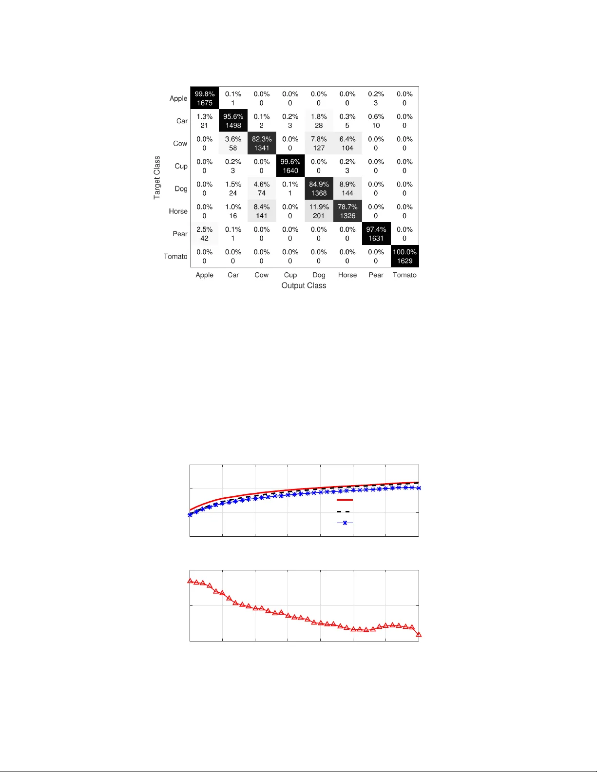
THE SUM OF TENSOR NETWORKS Giuseppe G. Calvi, Ilia Kisil, Danilo P . Mandic Electrical and Electronic Engineering Department, Imperial College London, SW7 2AZ, UK E-mails: { giuseppe.calvi15, i.kisil15, d.mandic } @imperial.ac.uk ABSTRA CT T ensor networks (TNs) have been gaining interest as multiway data analysis tools o wing to their ability to tackle the curse of dimensionality and to represent tensors as smaller -scale interconnections of their intrinsic features. Howe ver , despite the obvious adv antages, the current treatment of TNs as stand-alone entities does not take full benefit of their underlying structure and the associated feature localization. T o this end, embarking upon the analogy with a feature fusion, we propose a rigorous framew ork for the combination of TNs, focusing on their summation as the natural way for their combination. This allows for feature combination for any number of tensors, as long as their TN representation topologies are isomorphic. The benefits of the proposed framework are demonstrated on the classification of sev eral groups of partially related images, where it outperforms standard machine learning algorithms. Index T erms — Sum of tensor networks, T ucker decomposition, classification, feature e xtraction, graphs 1. INTR ODUCTION T ensors are multidimensional generalizations of matrices and vectors, and their ability to make enhanced use of data structures to perform dimensionality reduction and component extraction offers a po werful tool in the analysis of Big Data. Owing to their flexibility and a scalable way to deal with multi-way data, tensors have found application in a wide range of disciplines, from the most theoretical ones, such as mathematics and numerical analysis [1, 2, 3], to the more practical signal processing applications [4, 5]. Applying standard numerical methods to tensors may be difficult, as in the raw format the required storage memory and number of operations grow exponentially with the tensor order ( curse of dimensionality ) [6]. T o overcome this issue, tensor decompositions (TDs) hav e been introduced with the aim to represent tensors by a much smaller number of parameters, via multilinear operations over the latent factors. The most well-known TD approaches are the Canonical Polyadic [7, 8], the T ucker [9, 10], and the T ensor Train decompositions [6] (CPD, TKD, and TT respecti vely). Any TD can be considered as a special case of the more general concept of tensor networks (TNs), which represent a high order tensor as a set of sparsely interconnected core tensors and factor matrices [5]. In other words, TNs can be viewed as multi-core interconnections of features of the original tensor . The advantages of representing a tensor as a TN are: (i) TNs are perfectly suited to deal with the curse of dimensionality , as a high order tensor can be stored on different machines which deal with only the indi vidual cores, (ii) each core may be representati ve of specific characteristics of the underlying tensor , thus implying inherent feature extraction on the original data. Despite these advantages, open problems in practical design of TNs include: (i) the choice of the TD for a particular application, (ii) minimization of the number of the parameters necessary for the TN representation [6], and (iii) to the best of our knowledge, a rigorous frame work to combine TNs. In this work, we address the point (iii), by focusing on the issue of TN summation for TNs of the same topology . Summation is the most natural way to combine any two entities into a ne w one, and we postulate that a sum of multiple tensors (summands), in their TN format , preserves the underlying structure in the inherent features of the summands. In this way , the sum of TNs immediately yields another isomorphic TN, the cores of which are a combination of the corresponding cores of the summand TNs. The summation operator can hence be interpreted as a process of mixing features of the original tensors, howe ver , algorithms for tensor network summation are still in their infanc y . T o this end, we propose a novel frame work for the summation of TNs (and inherently any two or more tensors represented by TNs). This is achieved by simple block arrangements of the corresponding original cores. Leveraging on the very efficient way in which TNs represent large tensors in terms of the required storage and computation, and realizing that interconnections among the cores in a TN describe how data structures of the original tensors are intertwined, we explore the possibility to combine corresponding individual cor es of two TNs with the same topology in order to obtain a new TN , the cores of which carry both joint and individual information present in the original cores. Therefore, this is related to the recently introduced common feature extraction in [11], howe ver , unlike matrices, the proposed framew ork enables this to be performed on tensors of any order, with the only condition that the original tensors are represented as TNs with equiv alent topologies. Practical advantages of the proposed framework are demonstrated through an image classification application based on the ETH-80 dataset [12], whereby every dataset entry is represented as a TN, and their individual features are combined via our proposed framew ork. This allows for the extraction of the shared information in the original data, which is then fed to a Support V ector Machine algorithm (SVM), and attains an ov erall classification rate of 92 . 3% . The proposed frame work therefore opens up ne w perspectiv es on the manipulation of TNs, completely removing the preconception that they hav e to be treated as stand-alone entities, and offers a ne w av enue for their applications. 2. NO T A TION AND BA CKGROUND A tensor of order N is denoted by boldface underlined uppercase letters, X ∈ R I 1 ×···× I N , a matrix by boldface uppercase letters, X ∈ R J × K , a vector by boldface lowercase letters, x ∈ R N × 1 , and a scalar by italic lowercase letters, x ∈ R . Subscripts are generally described by indices n, i, j, k . An element in a N -th order tensor is denoted by x i 1 ,i 2 ,...,i N = X ( i 1 , i 2 , . . . , i N ) . Giv en an N -th order tensor X ∈ R I 1 ×···× I n ×···× I N and an M -th order tensor Y ∈ R J 1 ×···× J m ×···× J M , with I n = J m , their ( m, n ) -contraction product is Z = X × m n Y , where Z is an ( N + M − 2) -th order tensor (for more detail we refer to [13]). By con vention × n is equi valent to × 2 n , and is referred to as mode- n contraction. The mode- n unfolding of a tensor X rearranges its elements into a matrix, and is expressed as X ( n ) (see [14] for more details). The symbol ⊗ denotes the Kronecker product, ◦ the outer product, and || · || the Frobenius norm. A TN representation of a tensor X is denoted by a calligraphic bold letter , X . Finally , the operator vec ( · ) indicates vectorization of a tensor . 2.1. T ucker Decomposition The TKD is analogous to a higher order form of matrix factorization, and decomposes an original tensor X into a core tensor contracted by a factor matrix along each corresponding mode [9, 15, 16]. In the case of a 3 -rd order tensor X ∈ R I × J × K , the TKD is expressed as X = G × 1 A × 2 B × 3 C = Q X q R X r P X p g q rp a q ◦ b r ◦ c p (1) where G ∈ R Q × R × P and A ∈ R I × Q , B ∈ R J × R , C ∈ R K × P , while a TKD for an N -th order tensor is gi ven by X = G × 1 A (1) × 2 A (2) × 3 · · · × N A ( N ) (2) For conv enience, any tensor expressed in the form of (2), will be referred to as “in the TKD format”, ev en though the factors A ( n ) were not necessarily obtained via a TKD. The mode- n unfolding of a tensor in the TKD format is X ( n ) = A ( n ) G ( n ) ( A ( N ) ⊗ · · · ⊗ A ( n − 1) ⊗ A ( n +1) ⊗ · · · ⊗ A (1) ) T (3) 2.2. Background on T ensor Netw orks A decomposition of a tensor into multi-way linked core tensors and matrices leads to equations often in volving numerous contraction products, which can be cumbersome to write and hard to visualize. For this reason it is common to represent tensors diagrammatically [13], as in Fig. 1. An N -th order tensor can be represented as a node (circle) with as many edges (modes) as the tensor order . In TNs, contractions are designated by linking two common modes, called contraction modes, while “dangling” edges are physical modes of the represented tensor . = x = x I I = X I J I J = X J I K I J K Fig. 1 : Building blocks of TNs. Anticlockwise from the top-left: scalar , vector , matrix, and 3 -rd order tensor . Edges are called modes, and the associated label I , J, K , indicate their dimensionality . T wo e xamples of TNs are provided in Fig. 2, whereby any mode which is not a physical mode is a contraction mode. Nodes linked only to contraction modes are contraction nodes, whereas nodes linked to one or more physical mode are referred to as physical nodes. The “shape” of a TN is its topology , where the concept of topology is the same to the one adopted in Graph Theory [17]. Each node in a TN X can either represent a particular feature of the original tensor X (in case of physical nodes), or a model on how features are combined (in case of contraction nodes). It is clear that, giv en that TNs represent tensors of any order , without a framew ork for combining TNs, the problem of mixing features of individual cores, which subsequently allo ws for the extraction of the common features across the individual tensors, becomes difficult to address. This characteristic of “feature locality” inherent to the nodes of a TN is of fundamental importance. Therefore our main motiv ation for this work is to provide the missing link for TN summation via a combination of their corresponding cores, thus simultaneously performing a mixture of features. Fig. 2 : Examples of TNs (figure adapted from [13]). Left: a TN representing a 16 -th order tensor , with contraction nodes shown in blue, and physical nodes shown in green. Right: a TN representing a 32 -th order tensor , with contraction nodes shown in blue ( 3 -rd order) and orange ( 4 -th order), and physical nodes in green. 3. SUM OF TENSOR NETWORKS T o establish a framework of summation of two or more TNs, assume that the individual TNs: (i) have physical modes with equal dimensions, (ii) hav e the same topology . W e proceed by providing the definitions, the main conjecture, and specific propositions arising from the conjecture, followed by an outline of practical applications. Definition 1. A block tensor is a tensor that is arranged into sub-tensors called blocks , that is, its entries are tensors of the same or der but not necessarily of the same dimensionality . Definition 2. The superdiagonal of a block tensor X ∈ R I 1 ×···× I N is the collection of entries x i 1 ,i 2 ,...,i n , where i 1 = i 2 = · · · = i n . Conjecture 1. Consider two tensors X , Y ∈ R I 1 ×···× I N r epresented as TNs with equivalent topologies, but not necessarily with equivalent contracting modes, referr ed to as X and Y . The sum Z = X + Y can then be repr esented as a new TN, Z , with equivalent topology to X and Y . Its contraction nodes ar e in the form of a block tensor which is obtained by stac king the corr esponding contraction nodes of X and Y along its superdiagonal. The physical nodes of Z ar e obtained by stacking the corr esponding physical nodes of X and Y in such a way that the dimensionality of all contracting modes is incr eased but that of the physical modes is kept fixed. Proposition 1. Conjecture 1 holds for c hains of matrices. Pr oof. Consider Fig. 3 as a graphical representation of Conjecture 1, and suppose X = A 1 A 2 · · · A N , Y = B 1 B 2 · · · B N , where X , Y ∈ R I × J , and A n , B n ∈ R R n × R n +1 , with R 0 = I , R N = J . Define a ne w chain of matrices Z = C 1 C 2 · · · C N , where each C n is an arrangement of A n , B n according to Conjecture 1. By a direct inspection of Z , we obtain Z = C 1 C 2 · · · C N =  A 1 B 1   A 2 0 0 B 2  · · ·  A N − 1 0 0 B N − 1   A N B N  = A 1 A 2 · · · A n + B 1 B 2 · · · B n = X + Y (4) X I A 1 R 1 A 2 R 2 · · · R N − 2 A N − 1 R N − 1 A N J Y I B 1 L 1 B 2 L 2 · · · L N − 2 B N − 1 L N − 1 B N J Z I C 1 R 1 + L 1 C 2 R 2 + L 2 · · · R N − 2 + L N − 2 C N − 1 R N − 1 + L N − 1 C N J + = Fig. 3 : Graphical representation of a sum of matrices X and Y , expressed as a matrix chain. The matrices (nodes) C n are composed of the matrices A n and B n , which are arranged according to Conjecture 1, either through a concatenation (two horizontal subnodes) or a block-diagonal arrangement (two diagonal subnodes). Proposition 2. Conjecture 1 holds for any tensor e xpr essed in the TKD format. Pr oof. F or simplicity we here prove Proposition 2 for 3 -rd order tensors, but without loss of generality the result holds for any tensor order . Fig. 4 shows the tensors X , Y ∈ R I 1 × I 2 × I 3 in the TKD format, that is X = G x × 1 A x × 2 B x × 3 C x Y = G y × 1 A y × 2 B y × 3 C y (5) with respective TN representations X , Y . A ne w TN, Z , is obtained by combining X and Y according to Conjecture 1 (observ e Fig. 4), and the so represented tensor , Z , can be described by Z = G z × 1 A z × 2 B z × 3 C z (6) The task is to show that Z = X + Y . W e shall consider the mode- 1 unfolding, but the same procedure can be applied to any mode. Define A z =  A x A y  , and G z as an arrangement of G x and G y along the superdiagonal of G z , and consider K 1 = ( C x ⊗ B x ) T K 2 = ( C y ⊗ B y ) T (7) Upon performing the mode- 1 unfolding of X and Y according to (3), and combining the matrices X (1) , Y (1) in their TN form, then from Proposition 1 the resulting matrix, Z ∗ , can be described as Z ∗ =  A x A y   G x (1) 0 0 G y (1)   K 1 K 2  T (8) Therefore, in order to prove Proposition 2 it is sufficient to show that Z (1) = Z ∗ , where Z (1) is the mode- 1 unfolding of Z represented as in (6). T o this end, consider Z (1) = A z G z (1) ( C z ⊗ B z ) T =  A x A y  G z (1)   C x C y  ⊗  B x B y   T (9) For con venience, denote X , Y , G x , G y ∈ R 2 × 2 × 2 , and define G α (: , : , j ) = ˆ G α ( j ) , where α ∈ { x, y } . Hence G z (1) =  ˆ G x (1) 0 ˆ G x (2) 0 0 0 0 0 0 0 0 0 0 ˆ G y (1) 0 ˆ G y (2)  (10) W ithout loss of generality assume C x =  1 2 5 6  C y =  3 4 7 8  (11) to giv e  C x C y  ⊗  B x B y  = =   1 h B x B y i 2 h B x B y i 3 h B x B y i 4 h B x B y i 5 h B x B y i 6 h B x B y i 7 h B x B y i 8 h B x B y i   = U (12) Upon substituting G z (1) and U into (9) and making use of the sparse nature of (10), we arriv e at Z (1) = A z G z (1) U T =  A x A y   ˆ G x (1) ˆ G x (2) 0 0 0 0 ˆ G y (1) ˆ G y (2)      1 B T x 5 B T x 2 B T x 6 B T x 3 B T y 7 B T y 4 B T y 8 B T y     =  A x A y   G x (1) 0 0 G y (1)   K T 1 K T 2  =  A x A y   G x (1) 0 0 G y (1)   K 1 K 2  T = Z ∗ (13) X + R 1 R 2 R 3 I 1 I 2 I 3 G x A x B x C x Y = L 1 L 2 L 3 I 1 I 2 I 3 G y A y B y C y Z R 1 + L 1 R 2 + L 2 R 3 + L 3 I 1 I 2 I 3 G z A z B z C z Fig. 4 : Graphical sum of tensors X and Y in the TKD format. 4. EXPERIMENT AL RESUL TS Practical implications of the main contribution of this paper , that is, Proposition 2, were in vestigated in an image classification task based on the benchmark ETH-80 dataset. It consists of 3280 images, composed of 8 classes, 10 objects per class, 41 images per object. For our simulations, the images were downsampled to 32 × 32 pixels. Giv en the RGB format of the considered images, our dataset consists of 3 -rd order tensors X m ∈ R 32 × 32 × 3 , m = 1 , . . . , M (where M = 3280 ). For each image, X m , in the training set a TKD was performed by setting the size of the core tensors to R 1 = R 2 = R 3 = 3 . The factor matrices { A m , B m , C m } were scaled by η 1 3 , where η = || G m || , to regularize the contribution of features. This is equiv alent to normalizing the core tensor of each TKD decomposition to unit norm, without affecting the accuracy of the approximation. The scaled factor matrices { A m , B m , C m } were concatenated into the matrices { A d , B d , C d } . The SVD was subsequently applied and the first { R 1 , R 2 , R 3 } singular vectors were retained (we refer to this operator as tSVD( · )), which yielded matrices { A c , B c , C c } . Finally , for each image, X m , a new core tensor w as computed as ◦ G m = X m × 1 A T c × 2 B T c × 3 C T c (14) Equation (14) represents the projection of the data images onto the features common to the full dataset, implying that ◦ G m can be used for classification purposes. Their vectorized versions vec ( ◦ G m ) , m = 1 , . . . , M , were fed to a machine learning classifier in the form of an SVM (Gaussian kernel), which employed a one-vs-one (O V O) approach. During the testing stage, for each new element X ∗ , vec ( ◦ G ∗ ) was computed analogously and was classified according to the trained model, as summarized in Algorithm 1. Algorithm 1. Sum of TNs for image classification 1: Input: Dataset { X m } M m =1 , { R 1 , R 2 , R 3 } 2: for each element m in dataset do 3: X m = G m × 1 × A m × 2 B m × 3 C m 4: η = || G m || 5: A d =  A d η 1 3 A m  6: B d =  B d η 1 3 B m  7: C d =  B d η 1 3 C m  8: end for 9: A c = tSVD ( A d , R 1 ) 10: B c = tSVD ( B d , R 2 ) 11: C c = tSVD ( C d , R 3 ) 12: for each element m in dataset do 13: ◦ G m = X m × 1 A T c × 2 B T c × 3 C T c 14: end for 15: T rain classifier on { vec ( ◦ G m ) } M m =1 . The procedure outlined in Algorithm 1 was applied to the ETH-80 dataset, with 80% of the available images serving as randomly selected training data. The av erage of 20 realizations yielded an accuracy of 92 . 3% . Observe in Fig. 5 that all classes were classified with a hit-rate > 90% except for “Co w”, “Dog”, and “Horse”, which in the dataset indeed look similar (we refer to [12]). Fig. 5 : Confusion matrix of the classification algorithm, where 80% of the data was used for training. Performance comparisons were conducted against an SVM (Gaussian k ernel) applied directly to the vectorised images, and a tensor-based classification method which we refer to as “TKD-CONCA T”, which concatenates all members of ETH-80 in a 4 -th order tensor , performs a TKD, and retains the first 3 factor matrices, as outlined in [18]. The results are shown in Fig. 6 and suggest that a direct summation of TNs yields a physically meaningful mixture of features, offering enhanced cross accuracy . Importantly , our proposed algorithm outperformed the other methods, especially when a small amount of data is available for training, as shown in the bottom graph. 10 20 30 40 50 60 70 80 Percentage of data used for training 70 80 90 100 Accuracy rate (%) Sum of TNs SVM TKD-CONCAT 10 20 30 40 50 60 70 80 Percentage of data used for training 0 1.0 2.0 Diff. in accuracy rate (%) Fig. 6 : Classification results using the sum of TNs approach. T op: Accurac y rates. Bottom: Dif ference in accuracy between classification based on sum of TNs and standard SVM. 5. CONCLUSION W e hav e introduced a formalism behind the sum of tensor networks, and hav e validated the approach for chains of matrices ( 2 -nd order tensors) and, more generally , for tensors in the T ucker format. By employing the analogy between the sum of tensor network cores and a feature fusion, we have devised a ne w algorithm for image classification, which rests solely upon the the sum of tensor networks. Moreover , the proposed algorithm has been shown to exhibit a noticeable adv antage when only few training data are av ailable. T ests on the the ETH-80 dataset hav e attained an accuracy rate of 92 . 3% , and the proposed algo- rithm has been shown to outperform both standard Support V ector Machine and a related tensor-based classification approach. Generalisations of the proposed framew ork are the subject of ongoing work. 6. REFERENCES [1] J. G. McWhirter and I. Proudler , Mathematics in signal pr ocessing V . Oxford University Press, 2002. [2] L. de Lathauwer , B. D. Moor , and J. V ande walle, “On the best rank-1 and rank- ( R 1 , R 2 , ..., R N ) approximation of higher- order tensors, ” SIAM Journal on Matrix Analysis and Applications , vol. 21, no. 4, pp. 1324–1342, 2000. [3] ——, “A multilinear singular value decomposition, ” SIAM Journal on Matrix Analysis and Applications , vol. 21, no. 4, pp. 1253–1278, 2000. [4] A. Cichocki, “T ensors decompositions: new concepts for brain data analysis?” Journal of Contr ol, Measurement, and System Inte gration (SICE) , vol. 47, no. 7, pp. 507–517, 2011. [5] A. Cichocki, D. P . Mandic, A. H. Phan, C. F . Caiafa, G. Zhou, Q. Zhao, and L. D. Lathauwer , “T ensor decompositions for signal processing applications, ” IEEE Signal Processing Ma gazine , vol. 32, no. 2, pp. 145–163, 2015. [6] V . Oseledets, “T ensor-train decomposition, ” Society for Industrial and Applied Mathematics , vol. 33, no. 5, pp. 2295– 2317, 2011. [7] R. Bro, “P ARAF AC. Tutorial and applications, ” Chemometrics and Intelligent Laboratory Systems , vol. 38, no. 2, pp. 149–171, 1997. [8] L. de Lathauwer , “A link between the canonical decomposition in multilinear algebra and simultaneous matrix diagonal- ization, ” SIAM Journal on Matrix Analysis and Applications , vol. 28, no. 7, pp. 642–666, 2006. [9] L. R. T ucker, “Some mathematical notes on three-mode f actor analysis, ” Psychometrika , vol. 31, no. 3, pp. 279–311, 1966. [10] ——, “T ucker dimensionality reduction of three-dimensional arrays in linear time, ” SIAM Journal on Matrix Analysis and Applications , vol. 30, no. 3, pp. 939–956, 2008. [11] G. Zhou, A. Cichocki, Y . Zhang, and D. Mandic, “Group component analysis for multiblock data: common and indi vidual feature extraction, ” IEEE T ransactions on Neural Networks and Learning Systems , v ol. 27, no. 11, pp. 2426–2439, 2016. [12] B. Leibe and B. Schiele, “ Analyzing appearance and contour based methods for object categorization, ” in Pr oc. IEEE Confer ence on Computer V ision and P attern Recognition (CVPR03) , June 2003, pp. 409–415. [13] A. Cichocki, I. Oseledets, Q. Zhao, N. Lee, A. H. Phan, and D. Mandic, “T ensor networks for dimensionality reduction and large-scale pptimization. P art: 1 lo w-rank tensor decompositions, ” vol. 9, no. 4–5, pp. 249–429, 2016. [14] S. Dolgov and D. Savostyano v , “Alternating minimal ener gy methods for linear systems in higher dimensions, ” SIAM Journal on Scientific Computing , v ol. 36, no. 5, pp. A2248–A2271, 2014. [15] L. R. T ucker , “Implications of factor analysis of three-w ay matrices for measurement of change, ” in Pr oblems in Measur - ing Change , C. W . Harris, Ed. Madison WI: Uni versity of W isconsin Press, 1963, pp. 122–137. [16] ——, “The extension of factor analysis to three-dimensional matrices, ” in Contributions to Mathematical Psychology . , H. Gulliksen and N. Frederiksen, Eds. New Y ork: Holt, Rinehart and W inston, 1964, pp. 110–127. [17] R. T rudeau, Introduction to gr aph theory . Kent State Uni versity Press, 1993. [18] A. H. Phan and A. Cichocki, “T ensor decompositions for feature extraction and classification of high dimensional datasets, ” IEICE Nonlinear Theory and Its Applications , vol. 1, no. 1, pp. 37–68, 2010.