Tensor Valued Common and Individual Feature Extraction: Multi-dimensional Perspective

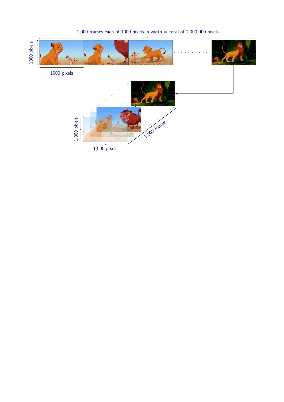
T ensor V alued Common and Individual F eature Extraction: Multi-dimensional P ersp ectiv e Ilia Kisil 1 , Giusepp e G. Calvi 1 , and Danilo P . Mandic 1 1 Electrical and Electronic Engineering Departmen t, Imp erial College London, SW7 2AZ, UK, E-mails: { i.kisil15, giusepp e.calvi15, d.mandic } @imperial.ac.uk No vem b e r 3, 2017 Abstract A no vel metho d for common and individual feature analysis from exceedingly large- scale data is proposed, in order to ensure the tractabilit y of both the computation and storage and th us mitigate the curse of dimensionality , a ma jor b ottlenec k in mo dern data science. This is achiev ed b y making use of the inherent redundancy in so-called multi-block data structures, whic h represent multiple observ ations of the same phenomenon taken at differen t times, angles or recording conditions. Up on providing an intrinsic link b et w een the properties of the outer vector pro duct and extracted features in tensor decompositions (TDs), the prop osed common and individual information extraction from multi-block data is p erformed through imp osing ph ysical meaning to otherwise unconstrained factorisation approac hes. This is sho wn to dramatically reduce the dimensionalit y of searc h spaces for subsequen t classification pro cedures and to yield greatly enhanced accuracy . Sim u- lations on a multi-class classification task of large-scale extraction of individual features from a collection of partially related real-world images demonstrate the adv an tages of the “blessing of dimensionalit y” asso ciated with TDs. Index terms— T ensor decomp osition, tensor rank, feature extraction, common and indi- vidual features, classification 1 In tro duction Mo dern datasets in data science applications ha ve immense v olume, v eracity , v elo cit y and v ariet y (the for V‘s of big data) [1, 2], and often exhibit a large degree of structural ric hness among their entries. These data characteristics are often prohibitive to the application of classical matrix algebra as its “flat-view” wa y of op eration cannot cop e with the sheer volume of data and the corresponding im balanced matrix structures, such as as “tall and narro w” or “short and wide” ones. On the other hand, when arranged in multi-dimensional structures (tensors), the same data often admit m uch more con venien t and mathematically tractable w ays of analysis, b y virtue of the associated m ulti-linear algebra. How ev er, un til recen tly , suc h an approach to data analysis was not v ery p opular, due to high demand for storage and computational resources. There are sev eral wa ys to tensorize data prior to further analysis, suc h as through: (i) natural tensor formation, (ii) exp erimen tal design, or (iii) mathematical construction [3]. This flexibilit y and a highly informativ e nature of m ulti-wa y data represen tation is supp orted by 1 Figure 1: Efficien t representation of an imbalanced blo c k-matrix structure (a set of video frames, top ro w) in the form of m uch more con venien t and flexible tensor structure (a cub e of frames, b ottom ro w). tensor decompositions (TDs) which allow for storage and memory efficien t lo w-rank appro xi- mation of otherwise intractable large data, and are b eing exploited in div erse range disciplines including brain science [4, 5], c hemometrics [6], psychometric [7], mac hine learning [8, 9] and signal pro cessing [3]. The generalisation of a matrix to a tensor, as in Fig. 1, is intuitiv e but highly non-trivial, not least due to multi-linear algebra ha ving differen t prop erties to linear algebra. Along these lines, the authors in [10] consider the physical meaning of factor matrices obtained through TDs. Missing data can also be handled through tensor dictionary learning [11], whereb y the tensor structure allo ws for a simultaneous retriev al of lo cal patterns and establishing the global information. The algorithms for classification of the multi-dimensional data hav e been prop osed in [12, 13]. W e here consider a problem of the extraction of information and classification of reduced di- mension features from large-scale m ulti-blo c k data. A typical example of such structure is a set of recordings of the same phenomenon but under differen t exp erimen tal setups, suc h as m ultiple images of ob jects recorded under different ligh ting and angle com bination, m ulti-blo c k data. In tuitively , the so obtained ensem ble of images con tains some common and some individual fea- tures, and mac hine learning tasks would b enefit from exploiting only either common features (for clustering) or individual features (for identification), b oth of m uch lo wer dimensionalit y than the original data. In this work, to resolve the computational and storage issues for large scale classification problems, the iden tification of common features is ac hieved by first pro viding an additional insigh t into the physical meaning of the outer pro duct of multiple v ectors in the tensor setting, supp orted by an intuitiv e example. The separation of the common and indi- vidual feature subspaces is then ac hiev ed by m ulti-linear rank decomp osition (LL1), whereb y the num b er of “simplest” data structures in suc h a decomp osition is equiv alent to the num b er of m ulti-linear tensor ranks [14]. The non-negativity constrain t is further imp osed on the so extracted factors, to preserve the physical properties of the images considered. Sim ulations on the b enc hmark ORL dataset demonstrate that the prop osed metho d pro vides significant 2 adv an tages in terms of accuracy , mathematical tractabilit y and ease of interpretation, when used in conjunction with standard classification algorithms. 2 Common and Individual Comp onen ts in Data Consider a set, X , of N observ ations in a matrix form, given by X = { X n ∈ R I × J n : n = 1 , 2 , . . . , N } (1) where the so called block-matrix structure X could b e a representation of medical images, EEG recordings, or financial sto c k c haracteristics. All members of suc h a set of matrices X are naturally linked together and it w ould b e b eneficial to analyse them simultaneously at the same time, ho w ever, the represen tation in (1) yields im balanced (tall and narro w) structure whic h is cumbersome for further pro cessing. The main goal of the common and individual feature analysis is, therefore, to mak e use of the “blessing of dimensionality” asso ciated with tensor structures, in order to find a m uc h low er-dimensional unique subspace ¯ A that is common across all n ∈ N . In this wa y , the common subspace, ¯ A , can b e separated from the individual information, ˘ A n , for ev ery n . The flat view matrix metho ds typically stac k all entries of X into a tall and narrow matrix X =  X T 1 , X T 2 , . . . , X T N  T and subsequently p erform matrix factorisations, suc h as the principal comp onen t analysis (PCA) [15], to give: X = ˘ A ¯ A T (2) where ˘ A =  ˘ A T 1 , ˘ A T 2 , . . . , ˘ A T N  T . In [16], this metho d w as applied to neuroimaging data of patien ts with Alzheimer disease, whereb y ¯ A is interpreted as well established knowledge ab out the disease (common components), while ˘ A n represen ts the individual state for a sp ecific pa- tien t. Ho wev er, as with all matrix models, this approac h do es not generalise w ell and is only appropriate when all comp onen ts, X n , of the tall and narrow matrix, X , exhibit exactly the same common information. Approac hes to common and individual feature extraction presented in [17, 18] also emplo y a PCA lik e factorisation to every entry of the naturally linked dataset given in (1), to yield X n = A n B T n = h ¯ A ˘ A n i " ¯ B T n ˘ B T n # = ¯ A ¯ B T n + ˘ A n ˘ B T n = ¯ X n + ˘ X n (3) where the matrices, ¯ X n , are the common comp onen ts across the dataset X , while the matrices, ˘ X n , are the individual comp onents for ev ery X n in X . The matrices ¯ A and ˘ A n are the basis matrices resp ectively for the matrices ¯ X n and ˘ X n , while the matrices, ¯ B n and ˘ B n represen t mixing co efficien ts so that ¯ X n = ¯ A ¯ B T n and ˘ X n = ˘ A n ˘ B T n Remark 1. Due to the linear separability of the matrices ¯ X n and ˘ X n , it is sufficien t to establish the basis of the common information, ¯ A , whic h can b e estimated through iterative minimisation of the cost function, form ulated in [19] as: J ( Q n , z ( n,m ) , a m ) = N X n =1   Q n z ( n,m ) − a m   2 F (4) where the orthogonal matrix Q n is obtained from X n = Q n R n , z ( n,m ) is the column vector of Z n = R n ( B T n ) † and a m is the common component whic h defines the basis of ¯ A , if the cost in (4) 3 Figure 2: The Canonical P olyadic Decomp osition (CPD). The tensor, X , is represen ted as a sum of rank-1 tensors, X r , giv en by the outer pro duct of the factor v ectors a r , b r , c r . is smaller then a predefined threshold. Th us, the w eak but consistently presented similarities among data matrices from the dataset X contribute to the total cost in (4) the s ame amoun t as the v ery prominent ones and, therefore, take imp ortant part in the multi-block data analysis. The matrix approac hes hav e their pros and cons and are p o werful if exploited appropriately , ho wev er, they do not account directly for the intrinsic m ultidimensional form of data. T o this end, w e prop ose a no v el metho d for common and individual feature extraction whic h exploits m ulti-mo dal prop erties of tensor decomp ositions. 3 Notation and Theoretical Bac kground A tensor of or der N is a N-dimensional arra y and is denoted b y a b old underlined capital letter, X ∈ R I 1 × I 2 ×···× I N . A particular dimension of X is usually referred to as a mo de . An element of a tensor is a scalar x i 1 ,i 2 ,...,i N = X ( i 1 , i 2 , . . . , i N ) which has N indices. A fib er is a v ector obtained b y fixing all but one of the indices, e.g. X ( i 1 , : ,i 3 ,...,i N ) is the mode-2 fib er. Fixing all but t wo of the indices yields a matrix called a slic e of a tensor, e.g. X ( : , : ,i 3 ,...,i N ) is the fr ontal slice. Mo de-n unfolding is the pro cess of element mapping from a tensor to a matrix, e.g. X → X (2) is the mo de-2 unfolding. A mo de-n pro duct of a tensor with a matrix is equiv alen t to Y = X × n A ⇔ Y ( n ) = AX ( n ) (5) The outer pro duct of N vectors results in a r ank-1 tensor of order N , e.g. a 1 ◦ a 2 ◦ · · · ◦ a n = X ∈ R I 1 × I 2 ×···× I N 3.1 Basic T ensor Decomp ositions The Canonical P olyadic Decomp osition (CPD), illustrated in Fig. 2, represents a given tensor X as a sum of rank-1 tensors X r , r = 1 , 2 , . . . , R . F or a third order tensor of rank R , the CPD is giv en by X ∼ = R X r =1 X r ∼ = R X r =1 λ r · a r ◦ b r ◦ c r ∼ = Λ × 1 A × 2 B × 3 C = J Λ ; A , B , C K (6) where Λ is a sup erdiagonal core tensor that guarantees “one to one relation” for the factor vec- tors a r , b r and c r , while A , B and C are factor matrices which are comp osed of the corresp ond- ing factor v ectors, e.g. A =  a 1 , a 2 , . . . , a R  . Despite soft uniqueness conditions, in practice the CPD in (6) do es not provide the exact decomp osition of the original data tensor [20]. On the 4 X O P Q = A 1 B T 1 c 1 + A 2 B T 2 c 2 + · · · + A K B T K c K Figure 3: The LL1 decomp osition is a combination of the CPD and the HOSVD. The tensor X k = ( A k B T k ) ◦ c k still exhibits the simplest structure within the LL1 decomp osition framew ork. other hand, the Higher Order Singular V alue Decomp osition (HOSVD) requires orthogonality constrain ts to b e imp osed on the factor matrices, is alwa ys exact [21], and takes the form X = R a X r a =1 R b X r b =1 R c X r c =1 g r a r b r c · a r a ◦ b r b ◦ c r c = G × 1 A × 2 B × 3 C = J G ; A , B , C K (7) where G is a dense core tensor, A , B , and C are the orthogonal factor matrices and the n-tuple ( R a , R b , R b ) is called the multi-line ar r ank . Observe that the HOSVD also decomp oses multi- dimensional data into a sum of rank-1 terms a r a ◦ b r b ◦ c r c . Ho w ever, as opp osed to the “one to one” relation for the CPD, the HOSVD mo dels all p ossible combinations of its factor vectors, hence, providing enhanced flexibility . T o make use of the desirable prop erties of b oth CPD and HOSVD, the LL1 decomp osition efficiently com bines their concepts [22], b y decomposing the tensor X in to a linear combination of K tensors, whereby each term X k = J Λ k ; A k , B k , c k K has a m ulti-linear rank ( L k , L k , 1), that is X = K X k =1 X k = K X k =1 ( A k B T k ) ◦ c k = K X k =1 G k ◦ c k = K X k =1 Λ k × 1 A k × 2 B k × 3 c k = K X k =1 G k × 3 c k (8) The LL1 decomp osition is illustrated in Fig. 3, where X ∈ R O × P × Q , and the “one to one” relation b etw een the factor matrices A k ∈ R O × L k , B k ∈ R P × L k , and factor vector c k ∈ R Q is preserv ed. Moreov er, upon emplo ying the matrix-tensor dualit y , w e can represen t the matrix G k ∈ R O × P as a tensor of order three, ˆ G k ∈ R O × P × 1 , so that ˆ G k = G k . Remark 2. The matrix G k in (8) is no longer of rank-1 and is consequently more informativ e. Ho wev er, the so-obtained tensor X k = G k ◦ c k is still considered to exhibit the simplest structure as far as the LL1 decomp osition is concerned. 4 Common and Individual F eature Extraction The intuition b ehind the prop osed common and individual feature analysis is giv en in the follo wing examples. Example 1. Observ e a rank-1 tensor of order 3, expressed as X = a ◦ b ◦ c = Y ◦ c with c = h 1 4 8 i T (9) According to the v alues of c and the definition of the outer product, the v alues in the first fron tal slice of X ( : , : , 1) are resp ectively four and eigh t times smaller then the v alues in the second 5 Color ensemble = rank-1 Red Base color 1 c R + rank-1 Green Base color 2 c G + rank-1 Blue Base color 3 c B Figure 4: Link b etw een the outer pro duct and common features for multidimensional data. The ensemble consists of the grey , yello w, magen ta, bright blue and brown-orange colors eac h of whic h is a combination of three base colors: red, green, blue. X ( : , : , 2) and third X ( : , : , 3) fron tal slices. Hence, eac h observ ation stored as the fron tal slice of X exhibits the same pattern (base matrix Y = a ◦ b ) that can b e considered as a common feature . A t this p oint, no individual information can b e extracted since there is only one base matrix. Example 2. Consider a collection, X , of five different color matrices stack ed along the third dimension, as illustrated in Fig. 4. The tensor rank of suc h a 3rd order tensor (color ensem ble) is three, that is, equiv alent to the num b er of base colors (red, green, blue), whic h are the simplest structures from whic h all data can b e generated through a mixing matrix C = [ c R , c G , c B ] ∈ R 5 × 3 . Th us, adopting the multi-lin ear notation and the R GB representation of colors, w e can write X = Λ × 1 A × 2 B × 3 C = Y × 3 C = Y ( : , : , 1) ◦ c R + Y ( : , : , 2) ◦ c G + Y ( : , : , 3) ◦ c B c R = h 128 256 256 0 256 i T c G = h 128 256 0 256 128 i T c B = h 128 0 256 256 32 i T (10) Here, X ∈ R I × J × 5 is the original data, and C = [ c R , c G , c B ] ∈ R 5 × 3 con tains in tensity v alues of the red, green and blue colors. These three base colors are stored in differen t rank-1 frontal slices of the tensor Y = Λ × 1 A × 2 B ∈ R I × J × 3 and represen t common information among the fron tal slices X ( : , : ,n ) . The individual features can be obtained by subtracting the weigh ted common features, to giv e ˘ X n = X n − ¯ X = X ( : , : ,n ) − X k ∈ K n α k Y ( : , : ,k ) (11) where K n is a subset of common features for X n with resp ect to the v alues in the n-th row of C . 4.1 LL1 decomp osition with non-negativit y constrain t If a slice Y ( : , : ,k ) b elongs to the set of common features for the data sample X ( : , : ,n ) , then an in tuitive implication is that the corresp onding v alue of C ( n,k ) is p ositive. Ho wev er, this cannot b e guaran teed for a general implemen tation of TDs, and the non-negativity constraint should b e imp osed on the factor matrix C , since it corresp onds to the mo de along whic h mem b ers 6 Algorithm 1. LL1 decomp osition with non-negativity constraint Input: X ∈ R O × P × Q and K sets of m ultilinear tensor rank ( L k , L k , 1) Output: F actor matrices A k ∈ R O × L k , B k ∈ R P × L k , c k ∈ R Q , and scaling v ectors λ k ∈ R L k 1: Initialize factor matrices A k , B k , c k 2: while not conv erged or iteration limit is not reached do 3: for k = 1, . . . , K do 4: X = X − P N n =1 ,n 6 = k J Λ n ; A n , B n , c n K 5: C k = rep eat( c k , L k ) 6: ˆ A k = X (1) ( C k  B k )( C T k C k ∗ B T k B k ) † 7: ˆ B k = X (2) ( C k  A k )( C T k C k ∗ A T k A k ) † 8: ˆ c k = NonNegLeastSq ( A  B , X (3) ) 9: Normalize eac h column of ˆ A k , ˆ B k and ˆ c k to unit length and store the norms in λ k 10: Assign ˆ A k → A k ; ˆ B k → B k ; ˆ C k → C k 11: end for 12: end while 13: return A k , B k , C k and λ k of the ensemble are stac k ed together. In order to obtain more descriptive common features, w e emplo y the LL1 decomp osition from (8). In this wa y , the rank of a frontal slice Y ( : , : ,k ) is increased (see Remark 2), whereb y the extraction of the common features is given by Y ( : , : ,k ) = A k B T k (12) and requires the minimization of the cost function min A k , B k , c k       X − K X k =1 J Λ k ; A k , B k , c k K       2 F s.t. c k > 0 (13) Notice that this problem is similar to the computation of the CPD in (6). Therefore, our solution is based on the ALS-CPD algorithm (w e refer to [20] for more detail) and is summarized in Algorithm 1, where ∗ and  denote respectively Khatri-Rao and Hadamard products, ( · ) † is the Mo oreP enrose pseudoinv erse, NonNegLeastSq( X , Y ) p erforms least squares on an input X and an output Y , the least squares coefficients are constrained to b e non-negative [23], while rep eat( X , n ) duplicates an input X n times. Remark 3. F or the illustration of the prop osed approach, we used a tensor of order three, ho wev er, unlike matrices the prop osed approach generalises w ell and allows for the common and individual features to b e extracted from a tensor of any order, with only one requirement that observ ations must b e concatenated along the same mo de. 5 Sim ulations and Analysis The prop osed approach was emplo yed for the classification of face images from the b enc hmark ORL dataset [24]. This database includes a total of the 400 grey scale images of 40 sub jects in ten differen t illumination conditions and facial expressions. T en sets of 40 images were created b y randomly choosing one image of ev ery sub ject. Six of these sets w ere arbitrarily selected for the training set with the remaining four forming the test set. Each group from the training set w as represented as a tensor X i ∈ R 112 × 92 × 40 where the images of 40 different sub jects were stac ked along the third dimension, as in Fig. 5. Their individual features were extracted b y applying the prop osed framew ork with the non-negativit y constrain t imp osed on the mo de-3 7 Original information Common information CPD LL1 Individual information (Original – Common LL1) Figure 5: Left column: Examples of the tensor represen tations for X i ∈ R 112 × 92 × 40 where the images of 40 differen t sub jects were stack ed along the third dimension during the training stage for tensor-based common and individual feature extraction. Righ t column: Common and individual feature extraction. Left: Examples of images in the ORL dataset. Cen ter: Examples of common features computed through the CPD and LL1 decomp ositions. Righ t: Examples of extracted individual features obtained by subtraction of the common information from the corresp onding original images. factor matrix, while the n umber of common features was found empirically . The classification mo dels used w ere SVM, NN, QD and cKNN and w ere trained on the so obtained individual information. The classification scores were calculated from 100 realizations. Note that during the test stage, w e used the original images in order to make a fair and realistic ev aluation. T able 1: Classification P erformance in % SVM NN QD cKNN Original 83.9 4.35 91.5 79.0 CPD 91.5 85.8 89.8 85.5 LL1 94.7 92.2 86.8 84.3 Fig. 5 illustrates examples of images used in the exp eriments, and the extracted individual information and common features for the CPD and LL1 decomp osition. T able 1 summarizes the p erformance of multi-class classification of the original images based on the corresp onding individual information, extracted through the prop osed metho d for the CPD and LL1 decom- p ositions. The most significant improv emen t can be observed for the NN based classifier. Here, the p o or accuracy on the original data is asso ciated with the high v ariance of the original samples and the small size of the training set whic h resulted in ov erfitting. On the other hand, the extracted individual features w ere of low er v ariance, whic h allo wed the NN classifier to find a decision b oundary that is less prone to fluctuations in the training data, leading to m uch higher classification accuracy . 6 Conclusion W e ha ve prop osed a nov el framework for common and individual feature extraction based on the CPD and LL1 tensor decomp ositions with the non-negativity constrain t. The m ulti- mo dal relations expressed through the outer pro duct ha ve b een sho wn to play a k ey role in the extraction of the shared information from m ulti-blo ck data. In this w ay , the p erformance of mac hine learning algorithms can b e greatly enhanced, as the classification mo dels use only the m uch lo w er dimensional and significan tly more discriminative individual information during 8 the training stage. Simulations hav e employ ed the ORL database of images taken from v arious angles, under sev eral illumination conditions, and with differen t face expressions of the sub jects and ha ve ac hiev ed excellent results. Unlike the matrix metho ds, the prop osed metho d is very flexible and is not restricted to input data of a sp ecific shared structure or images of the same dimensions. References [1] A. Cic ho c ki, “Era of big data pro cessing: A new approac h via tensor net w orks and tensor decomp ositions,” arXiv pr eprint arXiv:1403.2048 , 2014. [2] A. Cic ho cki, N. Lee, I. Oseledets, A. H. Phan, Q. Zhao, and D. P . Mandic, “T ensor net- w orks for dimensionality reduction and large-scale optimization. Part 1: Low-rank tensor decomp ositions,” F oundations and T r ends ® in Machine L e arning , vol. 9, no. 4-5, pp. 249–429, 2016. [3] A. Cichocki, D. P . Mandic, L. De Lathau w er, G. Zhou, Q. Zhao, C. Caiafa, and H. A. Phan, “T ensor decomp ositions for signal pro cessing applications: F rom t wo-w ay to multiw a y comp onen t analysis,” IEEE Signal Pr o c essing Magazine , v ol. 32, no. 2, pp. 145–163, 2015. [4] A. Cichocki, “T ensor decomp ositions: A new concept in brain data analysis?,” arXiv pr eprint arXiv:1305.0395 , 2013. [5] J. Escudero, E. Acar, A. F ern´ andez, and R. Bro, “Multiscale entrop y analysis of resting- state magneto encephalogram with tensor factorisations in Alzheimer’s disease,” Br ain R ese ar ch Bul letin , vol. 119, pp. 136–144, 2015. [6] A. Smilde, R. Bro, and P . Geladi, “Multi-w ay analysis: Applications in the chemical sciences,” T e cnometrics , pp. 1–380, 2005. [7] H. A. Kiers and I. V. Mec helen, “Three-wa y comp onent analysis: Principles and illustrativ e application,” Psycholo gic al Metho ds , vol. 6, no. 1, pp. 84–110, 2001. [8] N. D. Sidirop oulos, L. De Lathau wer, X. F u, K. Huang, Ev angelos E. P ., and C. F alout- sos, “T ensor decomp osition for signal pro cessing and machine learning,” arXiv pr eprint arXiv:1607.01668 , 2016. [9] T. D. Nguy en, T. T ran, D. Q. Ph ung, and S. V enk atesh, “T ensor-v ariate restricted Boltz- mann mac hines,” In Pr o c e e dings of the 29th Confer enc e on Artificial Intel ligenc e , pp. 2887–2893, 2015. [10] F. Cong, Q. Lin, L. Kuang, X. Gong, P . Astik ainen, and T. Ristaniemi, “T ensor decom- p osition of EEG signals: A brief review,” Journal of Neur oscienc e Metho ds , v ol. 248, pp. 59–69, 2015. [11] H . A. Phan, A. Cichocki, P . Ticha vsk ` y, G. Luta, and A. Bro ckmeier, “T ensor completion through m ultiple Kroneck er pro duct decomp osition,” In Pr o c e e dings of the 2013 IEEE International Confer enc e on A c oustics, Sp e e ch and Signal Pr o c essing (ICASSP) , pp. 3233– 3237, 2013. [12] B. Sa v as and L. Eld´ en, “Handwritten digit classification using higher order singular v alue decomp osition,” Pattern R e c o gnition , vol. 40, no. 3, pp. 993–1003, 2007. 9 [13] R. Zink, B. Hun y adi, S. V an Huffel, and M. De V os, “T ensor-based classification of an auditory mobile BCI without a sub ject-sp ecific calibration phase,” Journal of Neur al Engine ering , vol. 13, no. 2, pp. 1–10, 2016. [14] L. Sorb er, M. V an Barel, and L. De Lathauw er, “Optimization-based algorithms for tensor decomp ositions: Canonical p olyadic decomp osition, decomposition in rank-(L r ,L r ,1) terms, and a new generalization,” SIAM Journal on Optimization , vol. 23, no. 2, pp. 695– 720, 2013. [15] Y . Guo and G. P agnoni, “A unified framew ork for group indep endent comp onent analysis for m ulti-sub ject fMRI data,” Neur oImage , vol. 42, no. 3, pp. 1078–1093, 2008. [16] A . R. Grov es, C. F. Bec kmann, S. M. Smith, and M. W. W o olric h, “Linked indep endent comp onen t analysis for m ultimo dal data fusion,” Neur oImage , vol. 54, no. 3, pp. 2198– 2217, 2011. [17] E. F. Lo c k, K. A. Hoadley , J. S. Marron, and A. B. Nob el, “Join t and individual v ariation explained (JIVE) for in tegrated analysis of multiple data types,” The A nnals of Applie d Statistics , v ol. 7, no. 1, pp. 523–550, 2013. [18] G. Zhou, A. Cic ho c ki, Y. Zhang, and D. P . Mandic, “Group comp onen t analysis for m ultiblo c k data: Common and individual feature extraction,” IEEE T r ansactions on Neur al Networks and L e arning Systems , vol. 27, no. 11, pp. 2426–2439, 2016. [19] G. Zhou, A. Cichocki, and D. P . Mandic, “Common comp onen ts analysis via linked blind source separation,” In Pr o c e e dings of the 2015 IEEE International Confer enc e on A c oustics, Sp e e ch and Signal Pr o c essing (ICASSP) , pp. 2150–2154, 2015. [20] T. G. Kolda and B. W. Bader, “T ensor decomp ositions and applications,” SIAM R eview , v ol. 51, no. 3, pp. 455–500, 2009. [21] L. De Lathau wer, B. De Mo or, and J. V andewalle, “A m ultilinear singular v alue decomp o- sition,” SIAM Journal on Matrix Analysis and Applic ations , vol. 21, no. 4, pp. 1253–1278, 2000. [22] L. De Lathau w er, “Decomp ositions of a higher-order tensor in blo c k terms. Part I I: Defi- nitions and uniqueness,” SIAM Journal on Matrix A nalysis and Applic ations , vol. 30, no. 3, pp. 1033–1066, 2008. [23] D. D. Lee and H. S. Seung, “Algorithms for non-negative matrix factorization,” In Pr o c e e dings of the 2000 Confer enc e on A dvanc es in Neur al Information Pr o c essing Systems (NIPS) , pp. 556–562, 2001. [24] F. S. Samaria and A. C. Harter, “P arameterisation of a sto chastic mo del for human face iden tification,” In Pr o c e e dings of the Se c ond IEEE Workshop on Applic ations of Computer Vision , pp. 138–142, 1994. 10