Sound Source Localization in a Multipath Environment Using Convolutional Neural Networks

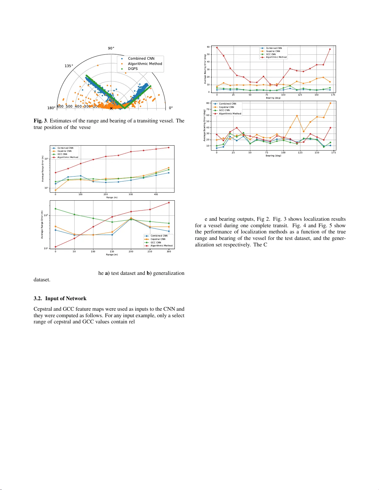
SOUND SOURCE LOCALIZA TION IN A MUL TIP A TH ENVIR ONMENT USING CONV OLUTION AL NE URAL NETWORKS Eric L. F er guson ∗ , Stefan B. W illi ams Australian Centre for Field Robotics The Univ ersity of Sydney , Australi a Craig T . Jin Computing and Audio Research Laboratory The University of Sydney , Aust ralia ABSTRA CT The propagation of sound in a shallo w water en vironme nt is cha rac- terized by boundary reflections from the sea surface and sea floor . These reflections result in multiple (indirect) sound propagation paths, which can degrade the performance of passiv e sound source localization method s. This p aper propose s the use of con volutional neural networks (CNNs) for the localization of sources of broad- band acoustic radiated no ise (such as motor v essels) in sh allo w water multipath en viron ments. It is shown that CNNs operating on cepstrogram and generalized cross-correlogram inputs are able to more reliably estimate the instantaneo us range and bearing of transiting motor vessels when the source localization performance of con v entional passiv e ranging methods is deg raded. T he ensuing improv ement in source localization performance is demonstrated using real data collected during an at-sea experiment. Index T erms — source localization, DOA estimation, con vo lu- tional neural networks, passiv e sonar , rev erberation 1. INTRODUCTION Sound source localization plays an important role in array signal pro- cessing with wide applications in communication , sonar and robotics systems [1]. It is a focal topic in the scientific lit erature on acous- tic array signal processing with a continuing challenge being acous- tic source l ocalization i n the presence of interfering multipath ar- riv a ls [2, 3, 4]. In practice, con ven tional passive narrowba nd sonar array methods in v olve frequency-domain beamforming of t he out- puts of hydrop hone elements in a receivin g array to detect weak sig- nals, resolve cl osely-spaced sources, and estimate the direction of a sound source. T yp ically , 10-100 sensors form a l inear array with a uniform interelement spacing of half a wav elength at the array’ s design frequency . Howe v er , this narrowba nd approach has applica- tion ove r a limited band of frequencies. The upper l imit is set by the design frequency , above which grating lobes form due to spatial aliasing, l eading to ambiguous source directions. The lo wer limit is set one octa v e belo w the de sign frequenc y because at lo wer f r equen- cies the directivity of t he array is much reduced as t he beamwidths broaden. An alternative approach to sound source l ocalization is to mea- sure the time difference of arriv al (T D OA) of t he signal at an ar- ray of spatiall y distrib uted receivers [5, 6, 7, 8], allowing the in- stantaneous position of the source to be estimated. The accuracy of the source position estimates i s found to be sensitiv e to any uncer- tainty i n the sensor positions [9]. F urthermore, rev erberation has an adverse ef fect on time delay estimation, which negati vely impacts ∗ W ork supported by Defence Science and T echno logy Group Austra lia. sound source localization [10]. In a model-based approach to broad - band source l ocalization in re verb erant en v ironments, a mod el of the so-called early refl ections (multipaths) is used to subtract the rev er- beration componen t from the signals. This decreases the bias in the source localization estimates [11]. The app roach adopted here uses a minimum nu mber of sen- sors (no more than three) to localize the source, not only in bear- ing, but also in range. Using a single senso r , the instantaneou s range of a broadba nd signal source is estimated using the cepstrum method [ 12 ]. This method exploits the interaction of the direct path and multipath arr iv als, which is observ ed in the spectrogram of the sensor output as a Lloyds mirror interference pattern [12]. Gener- alized cross-correlation (GCC) is used to measure t he TDOA of a broadband signal at a pair of sensors which enables estimations of the source bearing. Furthermore, adding another sensor so that all three sensor positions are collinear enables the source range to be estimated using t he two TDO A measurements from the two adjacent sensor pairs. The range estimate corresponds to the radius of curv a- ture of the sphe rical wav efront as it traverses the receiv er array . T his latter method is commonly referred to as passive ranging by wave- front curvature [13]. Ho we v er , its source localization performance can become problematic in multipath en vironmen ts when there is a large number of extrane ous peaks i n the GCC function attributed to the presence of multipaths, and when the direct path and multi path arriv a ls are unresolv able (resulting in TDOA estimation bias). Also, its performance degrades as the signal source direction moves awa y from the array’ s broadside direction and completely fails at endfire. Note t hat this is not the case wi t h the cepstrum method wit h it s om- nidirectional ranging performance being independent of source di- rection. Recently , Deep Neural Networks (DNN) based on supervised learning methods hav e been applied to acoustic tasks such as speech recognition [14, 15], terrain classification [16], and source localiza- tion tasks [17 ]. A challenge for supervised learning methods for source localization is their ability to adapt to acoustic co nditions that are different from the tr aining conditions. T he acoustic char- acteristics of a shallow water en vironme nt are non-stationary with high lev els of clutter, backgroun d noise, and multiple propagation paths making it a difficult en vironmen t for DNN methods. A CNN is proposed that uses ge neralized cross-co rrelation (GCC) and cepstral feature maps as inputs to estimate both t he range and bearing of an acoustic source passive ly in a shallow water en viron ment. The CNN method has an inherent advantage since it considers all GCC and cepstral values that are physically significant when estimating the source position. Other approaches inv olv- ing time delay estimation typically consider only a single valu e (a peak) in t he GCC or cepstogram. The CNNs are t r ained using real, multi-channel acoustic recordings of a surface vessel underway in a 0 1 0 0 2 0 0 3 0 0 Q u e f r e n c y ( m s) C e p str o g r a m 0 2 0 4 0 6 0 8 0 1 0 0 1 2 0 T i m e ( se c o n d s) - 1 . 0 - 0 . 5 0 .0 0 .5 1 .0 T i m e De l a y ( m s) C r o ss- c o r r e l o g r a m Fig. 1 . a) Cepstrogram for a surface ves sel as it transits over a single recording hydrophone located 1 m abov e the sea floor , and b) the correspondin g cross-correlogram for a pair of hydropho nes. shallo w water en vironm ent. CNNs operating on cepstrum or GCC feature map inputs only are also considered and their performances compared. The proposed model is sho wn to localize sources wi th greater performance than a con v entional passi ve sonar localization method which uses TDOA measurements. Generalization perfor- mance of the networks is t ested by ranging another vessel wit h differe nt radiated noise characteristics. The original contributions of this work are: • De ve lopment of a multi-task CNN for the passiv e localiza- tion of acoustic broadband noise sources in a shallow water en viron ment where t he range and bearing of the source are estimated jointly; • Range and bearing estimates are continuous, allowing for im- prov ed resolution in position estimates when compared to other passi ve localization networks which use a discretized classification approach [17, 18]; • A nov el loss function based on localization performance, where bearing estimates are constrained for additional net- work regularization when training; and • A unified, end-to-end network for passi v e localization in re- verberate en vironme nts with i mprov ed performance ov er tra- ditional methods. 2. A COUSTIC LOCALIZA TION CNN A neural network is a machine learning technique t hat maps the in- put data to a label or continuous value through a multi-layer non- linear architecture, and has been successfully applied to applications such as image and object classification [19, 20], hyperspectral pixel- wise classification [21] and t err ai n classification using acoustic sen- sors [16]. CNNs learn and apply sets of filters that span small re gions of the input data, enabling them to learn local correlations. 2.1. Architecture Since the p resence of a broadband acous tic source is readily ob- served in a cross-correlogram and cepstrogram, Fig. 1, it i s possible to create a unified ne twork for estimating the po sition of a vessel rel - ativ e t o a receiving hydropho ne array . T he network is divided into sections, Fig 2. The GCC CNN and cepstral CNN operate in parallel and serve as feature extraction networks for the GCC and cepstral feature map inputs respectiv ely . Next, the outputs of the GCC CNN dense: 256 dense: 256 dense: 256 dense: 256 dense: 256 dense: 256 GCC input cepstral input multichannel acoustic recording Range output Bearing output GCC CNN Cepstral CNN Combined CNN Fig. 2 . Network architecture for t he acoustic localization CNN and cepstral CNN are concatenated and used as inputs for the dense layers, which outputs a range and bearing estimate. For both the GCC CNN and cepstral CNN, the fi rst con v olu- tional layer filt ers the input feature maps with 10 × 1 × 1 kernels. The second con volution al layer takes the output of the first con v olu- tional layer as input and filters it with 10 × 1 × 48 k ernels. The third layer also uses 10 × 1 × 48 kernels, and is followed by two fully- connected layers. The combined CNN further contains two fully- connected l ayers that take the concatenated output v ectors from both of the GCC and cepstral CNNs as input. All the full y-connected lay- ers have 256 neurons each. A single neuron is used for regression output for the r ange and bearing outputs respectiv ely . All layers use rectified linear units as activ ation functions. Since resolution is im- portant for the accurate ranging of an acoustic source, max pooling is not used in the network’ s architecture. 2.1.1. Input In order to localize a source using a hydrophon e array , information about the time delay between si gnal propagation paths is required. Although such information is contained in the raw signals, it is ben- eficial to represent it i n a way that can be readily learned by the network. A cepstrum can be deri v ed from various spectra such as the complex or differential spectrum. For the current approach , the po wer cepstrum is used and is deriv ed from the power spectrum of a recorded signal. It is closely related to the Mel-frequency cepstrum used frequently in automatic speech recognition tasks [14, 15], but has linearly spaced frequency bands rather than bands approximating the human auditory system’ s response. The cepstral representation of the signal is neither i n the time nor frequency domain, but rather, it is in t he quefrency domain [ 22]. Cepstral analysis is based on the principle that the logarithm of the po wer spectrum for a signal containing echoes has an additi ve periodic component due to the echoes from multi -path reflections [23 ] . W here the original time wa veform contained an echo t he cepstrum will contain a peak and thus the TDOA between propagation paths of an acoustic signal can be measured by examining peaks in the cepstrum [24]. It i s useful in the presence of strong multipath reflections found in shallow water en vironments, where time delay estimation methods such as GCC suffer from degraded performance [25 ] . The cepstrum ˆ x ( n ) is obtained by the inv erse Fourier transform of the logarithm of the po wer spectrum: ˆ x ( n ) = F − 1  log | S ( f ) | 2  , (1) where S ( f ) is the Fourier transform of a discrete t ime signal x ( n ) . For a giv en source-sensor geometry , there i s a bounded range of quefrencies useful in source localization. As the source-sensor separation distance decreases, t he TDOA v alues (position of peaks in t he cepstrum) will tend to a maximum value, which occurs when the source is at the closest point of approach to the sensor . TDOA v alues greater than this maximum are not physically reali zable and are excluded . Cepstral value s near zero are dominated by source dependen t quefrencies and are also excluded. GCC is used to measure the TDO A of a signal at a pair of hydropho nes and is useful in situations of spatially uncorrelated noise [26]. For a giv en array geometry , there is a bounded range on useful GCC information. For a pair of recording sensors, a zero relativ e time delay corresponds to a broadside source, whilst a max- imum relativ e time delay corresponds to an endfire source. TDO A v alues greater than the maximum bou nd are not useful to the passiv e localization problem and are exclud ed [27, 12]. The windowing of CNN inputs has the added b enefit of reducing the number of pa- rameters in t he network. A cepstrogram and cross-correlogram (an ensemble of cepstrum and GCC respectively , as they v ary in time) is sho wn in Fig. 1. 2.1.2. Output For each example, the network predicts t he range and bearing of the acoustic source as a continuous value (each wit h a si ngle n euron regression output). This differs from other recent passiv e localiza- tion networks which use a classification based approach such that range and bearing predictions are discretized, putting a hard limit on the r esolution of estimations that the networks are able to pro- vide [17, 18]. 2.2. M ulti-task Jo i nt T rainin g The objectiv e of t he n etwork is to predict the range and bearing of an acoustic source relativ e to a recei ving array from rev erberant and noisy multi -channel input signals. Si nce the localization of an acoustic source in volv es both a range and bearing estimate, the Eu- clidean distance between the network prediction and ground truth is minimized when training. Both the range and bearing output loss componen t s are jointly minimized using a loss function based on lo- calization performance. This additional regularization i s expected to i mprov e localization performance when compared t o minimizing range loss and bearing loss separately . The t otal objectiv e function E minimized during network train- ing is giv en by the weighted sum of the polar-distance loss E p and the bearing l oss E b , such that: E = αE p + (1 − α ) E b , (2) where E p is the L 2 norm of the polar distance gi ven by: E p = y 2 + t 2 − 2 y t cos( θ − φ ) (3) and E b is the L 2 norm of the bearing loss only , giv en by: E b = ( θ − φ ) 2 (4) with the predicted range and bearing output denoted as t and φ re- specti vely , and the true range and bearing deno t ed as y and θ respec- tiv ely . The inclusion of the E b term encourages bearing predictions to be constrained to the first turn, providing additional regulariza- tion and reducing parameter weight magnitudes. The two terms are weighted by hyper-param eter α so each l oss term has roughly equal weight. T r ai ning uses batch normalization [28] and is stopped when the validation err or does not decrease appreciably per epoch. In or- der to further prev ent ov er-fitti ng, regularization through a dropout rate of 50 % is used in all fully connected layers when training [ 29]. 3. EXPERIMENT AL RESUL TS Passi ve localization on a transiting vessel was conducted using a multi-sensor algorithmic method described in [30], and CNN s with cepstral and/or GCC inputs. Their performances were then com- pared. The generalization ability of the netw orks to other broadband sources is also demonstrated by localizing an additional vessel w i th a different radiated noise spectrum and source level. 3.1. Dataset Acoustic data of a motor boat transiting in a shallow water en viron- ment over a hydrophon e array were recorded at a sampling rate of 250 kHz. The uniform linear array (ULA) consists of three reco rding hydropho nes with an interelement spacing of 14 m. Recording com- menced when the vessel was inbound 500 m fr om the sensor array . The vessel then transited ov er the array and recording was termi- nated when the vessel was 500 m outbound . The boat was equipped with a DGP S tracker , which logged its position relative to the re- cei ving hydrophone array at 0 . 1 s intervals. Bearing labels were wrapped between 0 and π radians, consistent with bearing estimates av ailable from ULAs which suf fer from left - r ight bearing ambiguity . T wenty-three transits were recorded ove r a two day period. One hun- dred thousand training examples were randomly chosen each wit h a range and bearing label, such that examp les uniformly distributed in range only . A further 50 00 labeled examp les were reserved for CNN training validation . The recordings were preprocessed as outlined in Section 2.1.1. T he network s were implemented in T ensorFlow and were tr ai ned with a Momentum Optimizer using a NVIDIA GeFo r ce GTX 770 GP U. The gradient descent was calculated for batches of 32 training examples. The networks were trained with a learning rate of 3 × 10 − 9 , weight decay of 1 × 10 − 5 and momentum of 0 . 9 . Additional recordings of the vessel were used to measure the perfor - mance of the methods. These recordings are referred t o as the test dataset and contain 9980 labeled examples. Additional acoustic data were recorded on a different day using a different boat with different radiated noise characteristics. Acous- tic recordings for each transit started when the inbound vessel was 300 m from the array , continued during its transit over the array , and ended when t he outbound vessel was 300 m away . This dataset is referred to as the generalization set and contains 11714 labeled examp les. 0 ° 4 5 ° 9 0 ° 1 3 5 ° 1 8 0 ° 2 2 5 ° 2 7 0 ° 3 1 5 ° 1 0 0 2 0 0 3 0 0 4 0 0 5 0 0 6 0 0 C o m b i n e d C NN Al g o r i t h m i c M e t h o d DG PS Fig. 3 . E stimates of t he range and bearing of a transiting vessel. The true position of the vessel is shown relativ e to the recording array , measured by the DGPS. 0 1 0 0 2 0 0 3 0 0 4 0 0 Ra n g e (m) 1 0 1 1 0 2 Av e rag e Ra n g e E r r o r (m) C o mb i n e d C NN C e p str a l C NN GC C C NN Al g o r i th mi c Me tho d 0 5 0 1 0 0 1 5 0 2 0 0 2 5 0 3 0 0 R a n g e (m ) 1 0 1 1 0 2 Av e r a g e Ra ng e E r r o r (m ) C o mb in e d C NN C e p str a l C N N GC C C NN A l g o r i th mi c M e t h o d Fig. 4 . Comparison of range estimation performance as a f unction of the vessels true range for the a) test dataset and b) generalization dataset. 3.2. Inp ut of Network Cepstral and GCC feature maps were used as inputs to the CNN and they were computed as follows. For any input example, only a select range of cepstral and GCC values contain relev ant TDOA informa- tion and are retained - see Secti on 2.1.1. Cepstral v alues more t han 1 . 4 ms are discarded becau se t hey represent the maximum multipath delay and occur when the source is directly over a sensor . Cepstral v alues less than 84 µ s are discarded since they are highly source de- pendent. Thus, each cepstrogram input is li ftered and samples 31 through 351 are used as input to the network only . A cepstral fea- ture vector is calculated for each recording channel, resulting in a 320 x 3 cepstal feature map. Due to array geometry , the maximum time de lay between pairs of senso r s is ± 9 . 2 ms. A GCC feature vec- tor is calcu l ated for two pairs of sensors, resulting i n a 4800 x 2 GCC feature map. T he GCC map is further sub-sampled to size 480 x 2 , which reduces the number of network parameters. 3.3. Comparison of Localization Methods Algorithmic passiv e localization was conducted using the methods outlined in [30]. The TDOA v alues required for algorithmic local- ization were taken from the largest peaks in the GCC. Nonsensical results at ranges greater than 1000 m are discarded. Other CNN ar- 0 2 5 5 0 7 5 1 0 0 1 2 5 1 5 0 1 7 5 Be ari n g (d e g ) 0 1 0 2 0 3 0 4 0 5 0 6 0 Av e rag e Be ari ng E r ro r (d e g ) C o mb i n e d C NN C e p s tr a l C NN GC C C NN Al g o r i th mi c Me th o d 0 2 5 5 0 7 5 1 0 0 1 2 5 1 5 0 1 7 5 Be a r i n g (d e g ) 1 0 2 0 3 0 4 0 5 0 6 0 7 0 8 0 Av e r a g e Be a r in g E r r o r ( d e g) C o mb in e d C NN C e p str a l C NN GC C C NN Al g or i th mic M e th o d Fig. 5 . Comparison of bearing estimation performance as a function of the vessels true bearing for the a) test da taset and b ) generalization dataset. chitectures are also compared. The GCC CNN uses the GC C CNN section of the combined C NN only , and the C epstral CNN uses the Cepstral CNN section of the combined CNN only , both with similar range and bearing outputs, Fig 2. Fig. 3 shows localization results for a vessel during one complete transit. Fig. 4 and Fig. 5 show the performance of localization methods as a function of the t rue range and bearing of the vesse l for the test dataset, and the gener- alization set respecti vely . The CNNs are able to localize a different vessel in the generalization set with some impact to performance. The performance of the algorithmic method is degraded i n the shal- lo w water en vironment since there are a l arge number of extraneous peaks in the GCC attributed to the presence of multipaths, and when the direct path and multipath arriv als become unresolv able (result- ing in TDO A estimation bias). Bearing estimation performance is improv ed in networks using GCC features, showing t hat time delay information between pairs of spatially distributed sensors is benefi- cial. The networks show improved robustness to interfering multi- paths. Range estimation performance is improv ed in networks using cepstral features, showing t hat multipath information can be useful in determining the sources range. The combined CNN is sho w n to provid e superior performance for range and bearing estimation. 4. CONCLUSIONS In this paper we i ntroduce t he use of a CNN for the localization of surface vessels in a shallow water en vironment. W e show that the CNN is able to jointly estimate the range and bearing of an acoustic broadband source in the presence of i nterferi ng multi paths. Sev- eral CNN architectures are compared and ev aluated. T he networks are trained and tested using cepstral and GCC feature maps as input deri ved from real acoustic r ecordings. Networks are tr ained using a nov el loss function based on localization performance wi th addi- tional constraining of bearing estimates. The inclusion of both cep- stral and GCC inputs facilitates robu st passi ve acoustic localization in re verberan t en vironments, where other methods can suffer f r om degrad ed performance. 5. REFERENCES [1] J. Benesty , J. Chen, and Y . Huang, Micr ophone array signal pr ocessing , vol. 1, Springer S cience & Business Media, 2008. [2] M. V iberg, B. Ottersten, and T . Kailath, “Detection and esti- mation in sensor arrays using weigh ted subsp ace fitting, ” IEE E T rans. Sign al Proc ess. , vol. 39, no. 11, pp. 2436–2449, 1991. [3] X. Zeng, M. Y ang, B. Chen, and Y . Jin, “Low angle direction of arriv al estimation by time re versal, ” in Proc. IEEE Int. Conf. Acoust., Speec h, Signal Proc ess. IEEE, 2017, pp. 3161–316 5. [4] J. Capon, “High-resolution frequency-w avenumbe r spectrum analysis, ” Pro c. IEEE , vol. 57, no. 8, pp. 1408–1418, 1969. [5] G.C. Carter, “T ime delay estimation for passi ve sonar signal processing, ” IEEE T rans. Acoust., Speec h, Signal Process. , vol. 29, pp. 463–470, 1981. [6] G.C. Carter, Ed., Coher ence and time delay estimation , IEEE Press, New Y ork, 1993. [7] Y .T . Chan and K . C. Ho, “ A simple and ef ficient estimator for hyperbolic location, ” IEEE T rans. on Signal Proce ss. , vol. 42, pp. 1905–191 5, 1994. [8] J. Benesty , J. Chen, and Y . Huang, “T ime-delay estimation via linear interpolation and cross correlation, ” IEEE T rans. Sp eech and Aud io Pr ocess. , vol. 12, no. 5, pp. 509–519, 2004. [9] E.L. F erguso n, “ Application of passive ranging by wavefro nt curv ature methods to the localization of biosonar click signals emitted by dolphins, ” i n Proc . of International Conf. on Un- derwater Acoust. Measur ements , 2011. [10] J. Chen, J. Benesty , and Y .A. Huang, “Performance of GCC- and AMDF-based time-delay estimation in practical rev erber- ant env ironments, ” EURASIP J . on Adv . in Signal Proces s. , vol. 2005 , no. 1, pp. 498964, 2005. [11] J.R. Jensen, J.K. Nielsen, R. Heusdens, and M.G. Christensen, “DO A estimation of audio sources in rev erberant en viron- ments, ” i n Proc. IEEE Int. Conf. Acoust., Speech, Signal Pro- cess. IEEE, 2016, pp. 176–180. [12] E.L. Ferguson, R. Ramakrishnan, S.B . Williams, and C .T . Jin, “Con volutional neural netwo r ks for passive monitoring of a shallo w water en vironment using a si ngle sensor , ” in Pro c. IEEE Int. Conf. A coust., Speech , Signal Pro cess. IEEE, 2017, pp. 2657–266 1. [13] E.L. F erguso n, “ A modified wave front curva ture method for the passi ve ranging of echolocating dolphins in the wild, ” J. Acoust. Soc. Am. , vol. 134, no. 5, pp. 3972–3972, 2013. [14] X. Xiao, S. W atanabe, H . Erdogan, L. Lu, J. Hershey , M.L. Seltzer , G. Chen, Y . Zhang, M. Mandel, an d D. Y u, “Deep beamforming networks for multi-channel speech recognition, ” in Proc. I EEE Int. Conf. Acoust., Speech, Signal Pro cess. IEEE, 2016, pp. 5745–57 49. [15] J. Heymann, L. Drude, Christoph Boeddeker , Patrick Hane- brink, and R. Haeb-Umbach, “Beamnet: end-to-end training of a beamformer-supported multi- channel asr system, ” in Pr oc. IEEE Int. Conf. A coust., Speech , Signal Pro cess. IEEE, 2017, pp. 5325–532 9. [16] A. V alada, L . Spinello, and W . Burgard, “Deep feature learn- ing for acoustics-based terrain classification, ” in Robotics Re- sear ch , pp. 21–37. Springer , 2018. [17] S. Chakrabarty and E.A.P . Habets, “Broad band DO A estima- tion usin g con volutional neural networks trained with noise signals, ” arXiv pr eprint arXiv:1705.009 19 , 2017. [18] R. T akeda and K. K omatani, “Unsupervised adap t ation of deep neural networks for sound sourc e localization using entropy minimization, ” in Pr oc. IEEE Int. Conf. Acoust., Speech, Sig- nal Pr ocess. IEEE, 2017, pp. 2217–2221. [19] A. Krizhevsk y , I. S utske ver , and G.E. Hinton, “Imagenet clas- sification with deep con volutional neural networks, ” in A dv . in neura l information proc ess. systems , 2012, pp. 1097–1105 . [20] R. Gir shick, J. Donahue, T . Darrell, and J. Malik, “Rich fea- ture hierarchies for accurate ob ject detection and semantic se g- mentation, ” in Proc. IEEE Con f. Computer V ision and P att ern Recog . , 2014, pp. 580–587. [21] L. W indrim, R. R amakrishnan, A. Melkumyan, and R. Mur- phy , “Hyperspectral CNN classification with l imited training samples, ” in B ritish Mac hine V ision Conf. , 2017. [22] B.P . Bogert, “The quefren cy alanysis of time series for echoes: Cepstrum pseudo-autoco variance, cross-cepstrum, and saphe cracking, ” T ime Series Analysis , pp. 209–243, 1963. [23] K.W . Lo, B.G. F erguso n, Y . Gao, and A. Maguer , “ Aircraft flight parameter estimation using acoustic multipath delays, ” IEEE T rans. o n Aer ospace and Electr onic S ystems , vol. 39, no. 1, pp. 259–268, 2003. [24] A.V . Oppenheim and R.W . Schafer , “F r om frequency to que- frency: a history of t he cepstrum, ” IEE E Sign al Pro cess. Ma g- azine , vol. 21, no. 5, pp. 95–106, 2004. [25] Y . Gao, M. Clark, and P . Cooper , “T ime delay estimate us- ing cepstrum analysis in a shallo w littoral en vironment, ” Conf. Underse a Defence T echnolo gy , vol. 7, pp. 8, 2008. [26] C. Knapp and G. Carter , “The generalized correlation method for esti mati on of t i me delay , ” IEEE T rans. A coust., Speech, and Signal Pr ocess. , vol. 24, no. 4, pp. 320–327 , 1976. [27] E.L. F erguso n, R. R amakrishnan, S.B. Williams, and C.T . Jin, “Deep learning approach to passiv e monitoring of the under- water acoustic en vironment, ” J. Acoust. Soc. Am. , v ol. 140, no. 4, pp. 3351–3351, 2016. [28] S. Ioffe and C. Szegedy , “Batch normalization: Accelerating deep network training by reducing internal cov ariate shift, ” in International Conf. o n Machine Learning , 2015, pp. 448–45 6. [29] N. Sriv astav a, G.E. Hinton, A. Kri zhe vsky , I . Sutskev er , and R. S alakhutdino v , “Dropout: a simple way to prev ent neural networks from overfitting., ” J . Machine Learning Resear ch , vol. 15, no. 1, pp. 1929–19 58, 2014. [30] H.C. Schau and A.Z. Robinson, “Passiv e source localization employ ing intersecting spherical surfaces fr om time-of-arriv al differe nces, ” IE EE T rans. on Acous t., Speec h, Signal Pr ocess. , vol. 35, no. 8, pp. 1223–12 25, 1987.