Dynamic Model Averaging for Practitioners in Economics and Finance: The eDMA Package

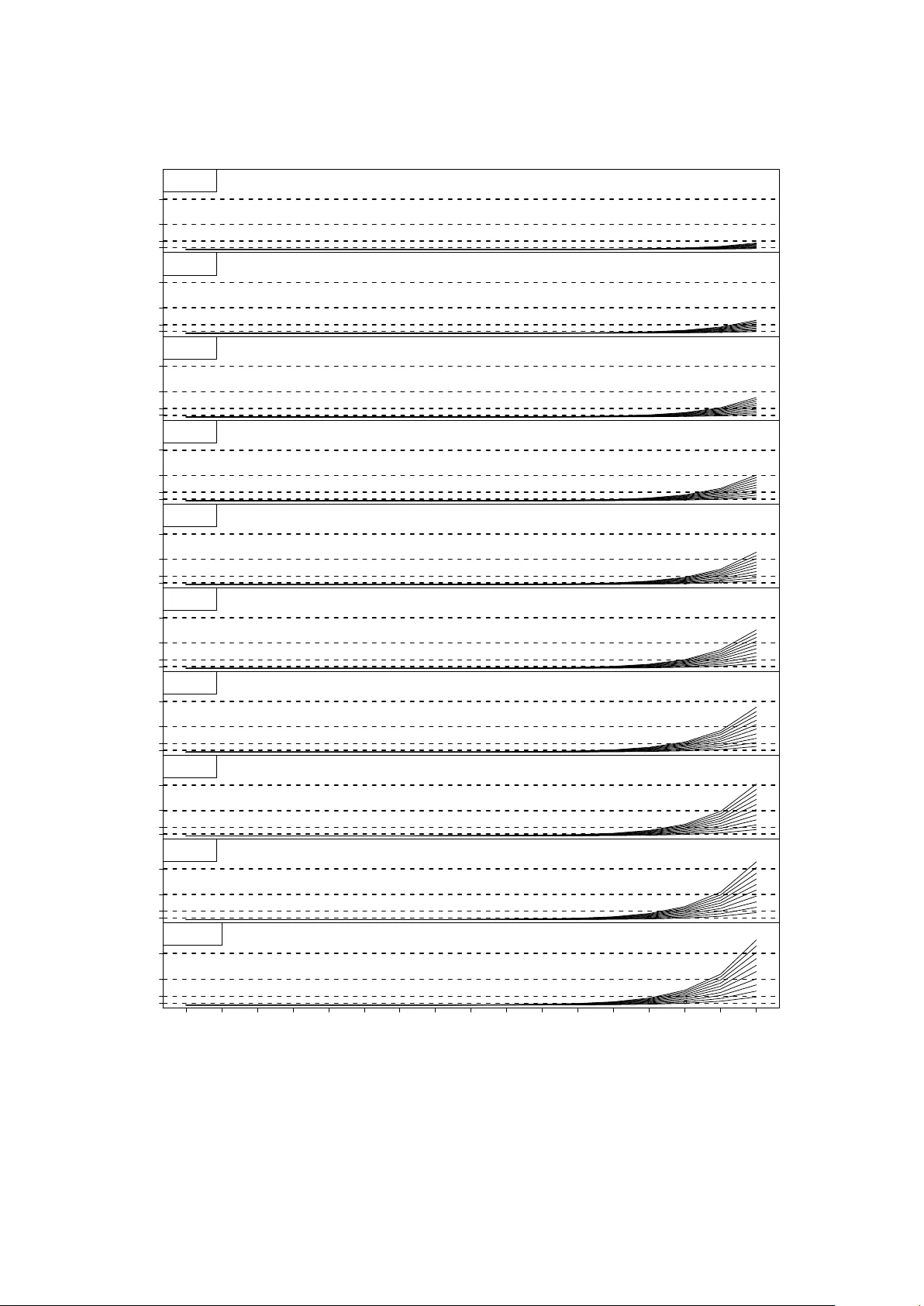
Dynamic Mo del Av eraging for Practitioners in Economics and Finance: The eDMA P ac k age Leop oldo Catania Univ ersity of Rome, “T or V ergata” Nima Nonejad Aalb org Univ ersity and CREA TES Abstract Raftery , K´ arn` y, and Ettler ( 2010 ) introduce an estimation technique, whic h they refer to as Dynamic Mo del Averaging (DMA). In their application, DMA is used to predict the output strip thickness for a cold rolling mill, where the output is measured with a time dela y . Recen tly , DMA has also sho wn to b e useful in macroeconomic and ﬁnancial appli- cations. In this pap er, we present the eDMA pac k age for DMA estimation implemen ted in R . The eDMA pac k age is esp ecially suited for practitioners in economics and ﬁnance, where typically a large n umber of predictors are av ailable. Our implementation is up to 133 times faster then a standard implemen tation using a single–core CPU. Th us, with the help of this pack age, practitioners are able to p erform DMA on a standard PC without resorting to large clusters, whic h are not easily av ailable to all researchers. W e demon- strate the usefulness of this pack age through simulation experiments and an empirical application using quarterly U.S. inﬂation data. Keywor ds : Dynamic mo del av eraging, Multi core CPU, Parallel computing, R , OpenMP . 1. In tro duction Mo del ing and forecasting economic v ariables such as real GDP , inﬂation and equit y premium is of clear imp ortance to researchers in economics and ﬁnance. F or instance, forecasting inﬂation is crucial for central banks with regards to conducting optimal monetary policy . Similarly , understanding and predicting equit y premium is one of the most widely imp ortan t topics discussed in ﬁnancial economics as it has great implications on p ortfolio choice and risk management, see for instance Dangl and Halling ( 2012 ) among many others. In order to obtain the best forecast as p ossible, practitioners often try to tak e adv antage of the many predictors av ailable and seek to com bine the information from these predictors in an optimal wa y , see Sto c k and W atson ( 1999 ), Sto c k and W atson ( 2008 ) and Groen, Paap, and Rav azzolo ( 2013 ) just to mention a few references. Recently , in the context of forecasting U.S. and UK inﬂation, Ko op and Korobilis ( 2011 ) and Ko op and Korobilis ( 2012 ), implement a tec hnique developed b y Raftery et al. ( 2010 ), referred to as Dynamic Model Aver aging (DMA). The original purp os e of the DMA in tro duced in Raftery et al. ( 2010 ) is more orien ted to wards engineers. Particularly , their aim is to predict the output strip thic kness for a cold rolling mill, where the output is measured with a time delay . D MA consists of many time– v arying co eﬃcien t regression mo dels formed from all p ossible com binations of the predictors a v ailable to a practitioner. Moreo ver, b esides allo wing for time–v ariation in the regression co eﬃcie n ts, int erpreting inclusion probabilities of each individual mo del, DMA also allows 2 eDMA : Eﬃcient Dynamic Mo del Averaging the relev ant mo del set to change with time as w ell through a forgetting factor. This w a y , past mo del p erform ance receives relatively less we igh t than current mo del p erformance and the estimation pro cedure adapts b etter to the incoming data. Koop and Korobilis ( 2011 ) and Ko op and Korobilis ( 2012 ) argue that b y sligh tly adjusting the original framework of Raftery et al. ( 2010 ), DMA can b e useful in economic applications, esp ecially inﬂation forecasting. 1 Dangl and Halling ( 2012 ) provide further suggestions on ho w to impro v e DMA such that it can b etter adapt to the patterns typically observ ed in economic and ﬁnancial data. The aforemen tioned authors, also pro vide a useful v ariance decomposition sc heme using the output from the estimation pro cedure . Byrne, Korobilis, and Rib eiro ( 2017 ), among others, use the modiﬁcations proposed in Dangl and Halling ( 2012 ) to model currency exchange–rate b eha vior. W e must also emphasize that DMA is not solely limited to these series and can b e used in a wide range of economic applications suc h as: F orecasting realized v olatilit y as w ell as house, oil and commo dit y prices. Ho wev er, from a practical p oin t of view, designing an eﬃcien t DMA algorithm r emains a c hal- lenging issue. As we demonstrate in Section 3 , DMA considers all p ossible combinations of predictors and forgetting factor v alues at eac h time–p eriod. T ypically , man y candidate v ari- ables are a v ailable and, as a consequence, it p oses a limit given the computational facilities at hand, which for many practitioners typic ally consists of a standard 8 core CPU. In most cases, av eraging o ver a relatively small num b er of mo d el combinations (usually b et ween 1000 to 3000) allo ws one to p erform DMA using standard lo ops and soft w are. How ev er, handling larger num b er of com binations can quickly b ecome v ery cum b ersome and imp ose technica l limits on the softw are at hand, esp ecially with regards to memory consumption, see for exam- ple, Ko op and Korobilis ( 2012 ). In order to deal with this issue, Onorante and Raftery ( 2016 ) suggest a strategy that considers not the whole mo del space, but rather a subset of mo dels and dynamically optimizes the choice of mo dels at each p oin t in time. How ev er, Onorante and Raftery ( 2016 ) hav e to assume that mo dels do not c hange to o fast o ver time, which is not an ideal assumption when dealing with ﬁnancial and in some cases mon thly economic data. F urthermore, it is not clear to us how one can incorp orate the mo diﬁcations suggested in Dangl and Halling ( 2012 ) within the framework of Onorante and Raftery ( 2016 ). In this pap er, we in tro duce the eDMA pack age for R ( R Core T eam 2016 ), whic h eﬃciently implemen ts a DMA pro cedure based on Raftery et al. ( 2010 ) and Dangl and Halling ( 2012 ). The routines in the eDMA pac k age are principally written in C++ using the armadillo library of Sanderson ( 2010 ) and then made av ailable in R exploiting the Rcpp and RcppAr- madillo pack ages of Eddelbuet tel, F ran¸ cois, Al laire, Ushey , Kou, Bates, and Chambers ( 2016a ) and Eddelbuettel, F ran¸ cois, and Bates ( 2016b ), resp ecti v ely . F urthermore, the OpenMP API ( Op e nMP 2008 ) is used to sp eedup the computations when a shared memory multiple pro- cessors hardw are is av ailable, which, now adays , is standard for the ma jorit y of commercial laptops. How ever, if the hardware do es not ha ve multiple pro cessors, the eDMA pack age can still b e used with the classical sequen tial CPU implementation. Our aim is to provide a pack- age that can b e used by a broad audience from diﬀerent academic ﬁelds who are in terested in implemen ting DMA in their research and obtain quan tities suc h as: Inclusion probabilities, out–of–sample forecasts or to p erform v ariance decomp osition. F urthermore, our pack age en- ables practitioners, to p erform DMA using a large n umber of predictors without needing to understand and possibly impleme n t complex programming concepts suc h as “ho w to eﬃciently 1 Speciﬁcally , Ko op and Korobilis ( 2012 ) change the conditional vola tilit y formula of Raftery et al. ( 2010 ) arguing that the original formula is not suited for the analysis of economic data. Leop oldo Catania, Nima Nonejad 3 allo cat e memory” , or “how to eﬃcien tly parallelize the computations” . It is also worth noting that, within the R envi ronmen t, the dma pac k age of McCormick, Raftery , and Madigan ( 2016 ) downloadable from CRAN can b e used to p erform the DMA of Raftery et al. ( 2010 ). Ho wev er, dma has several weaknesses such as (i): It do es not allow for the extensions mentioned in Dangl and Halling ( 2012 ), whic h are imp ortan t in the con text of in terpreting the amoun t of time–v ariation in the regression coeﬃcient s and performing a v ariance decomposition analysis, (ii): It is slo w compared to the pack age introduced in this pap er, (iii): It requires a v ery large amount of RAM when executed for mo deratel y large applications, and (iv): It does not allo w for parallel computi ng. W e refer the reader in terested in these asp ec ts to Section 5 , where w e rep ort a comparative analysis b et ween dma and eDMA using sim ulated data. Moreo ver, eDMA p er mits us to also p erform Bay esian Mo del Av eraging (BMA) and Bay esian Model Selection (BMS) for linear regression mo dels with constan t co eﬃcien ts implemented, for example, in the R pack ages BMA ( Raftery , Ho eting, V olinsky , Pain ter, and Y eung 2015 ) and BMS ( Zeugner and F eldkircher 2015 ). A t the same time, we obtain quan tities suc h as: Posterior inclusion probabilities and av erage mo del size, whic h allo w us to compare DMA (as well as Dyn amic Mo del Selection, DMS) with BMA (BMS) with regards to mo del shrink age and the magnitude of v ariation in the av erage mo del size. The structure of this pap er is as follows: Sections 2 and 3 brie ﬂy in tro duce DMA and its extensions. Section 4 presents the tec hnical asp ects. Section 5 provid es an intuiti v e description of the c hallenges that DMA p osses from a computat ional p oin t of view and prop oses solutions. Section 6 pro vides an empirical application to demonstrate the adv ant ages of eDMA from a practical p oint of view. Therefore, practitioners who are solely interested on how to implemen t DMA using the eDMA pack age can skip Sections 2 and 3 . Finally , Section 7 concludes. 2. F ramew ork Man y forecasting applications are based on a mo del where the v ariable of interest at time t , y t , dep ends on exogenous predictors and p ossibly lagged v alues of y t itself. F or instance, in panel (a) of Figure 1 , we plot the quarterly U.S. inﬂation rate, 100 4 ln P t , where P t denotes the U.S. Gross Domestic Pro duct implicit price deﬂator (GDPDEF) from 1968q1 to 2011q2. W e then recursiv ely ( i.e. , using data up to time t ) esti mate an autoregressiv e mo del of order 2, AR(2), of y t and rep ort the sum of the autoregressive co eﬃcient s, which can b e considered as a basic measure of inﬂation p ersistence in Panel (b). Our general conclusions from panels (a)–(b) are: Inﬂation is p ersistent and generally tends to b e higher during recessions than tranquil perio ds. It do es not appear to follo w an ident ical cyclical pattern either. F or example, inﬂation increases less aggressively tow ards the Great Recession of 2008 than the corresponding do wnturns in the 1970s, 1980s or the early 2000s. F urthermore, ev en in this simple mo del, we still observe some time–v ariation in the AR co eﬃcients. W e then extend the plain AR(2) mo del to also include the lagged unemploy men t rate (UNEMP) as a regressor. This w ay , we end up with a basic Philips curv e. In panel (c), we rep ort the recursive OLS estimates of UNEMP and in panel (d), w e rep ort the recursiv e p–v alues asso ciated to the null hypothesis that this estimate is equal to zero. Panel (d) shows that the unemplo yment rate in some p erio ds seems to b e a useful predictor of inﬂation. Results from panels (a)–(d) of Figure 1 suggest that tw o c hannels can potentially help to 4 eDMA : Eﬃcient Dynamic Mo del Averaging −1.00 0.00 1.00 2.00 3.00 4.00 (a) 0.80 0.86 0.92 0.98 1.04 1.10 (b) 1968 1973 1978 1983 1988 1993 1998 2003 2008 −0.50 −0.40 −0.30 −0.20 −0.10 0.00 (c) 0.00 0.16 0.32 0.48 0.64 0.80 (d) 1968 1973 1978 1983 1988 1993 1998 2003 2008 Figure 1: Panel (a): Quarterly GDPDEF inﬂation from 1968q1 to 2011q2. Panel (b): Inﬂation p ersistence estimates from an AR(2) mo del. P anel (c): Recursiv e OLS estimates of, θ 4 , in y t = θ 1 + θ 2 y t − 1 + θ 3 y t − 2 + θ 4 UNEMP t − 1 + e t , where e t ∼ N  0 , σ 2  . P anel (d): Recursive p –v alues for the null hypothesis of θ 4 = 0 at the 5% level. The gra y v ertical bars indicate business cycle p eaks, i.e. , the point at whic h an economic expansion transitions to a recession, based on National Bureau of Economic Research (NBER) business cycle dating. Leop oldo Catania, Nima Nonejad 5 impro ve the accuracy of inﬂation forecasts, (i): Incorp orating time–v ariation in the regression co eﬃcien ts. (ii): Augmen ting the AR mo del with exogenous predictors that can capture information b eyond that already contained in lagged v alues of y t . Th us, in many economic applications, we even tually end up with a mo del suc h as: y t = θ 1 t + θ 2 t y t − 1 + θ 3 t y t − 2 + θ 4 t x t − 1 + ... + θ nt z t − 1 + ε t , ε t ∼ N (0 , V t ) . (1) Ob viously , n can b e large and as a consequence, w e ma y hav e to deal with a ve ry large n umber of mo del combi nations. F or example, if our set of mo dels is deﬁned by whether each of the n p otential predictors is included or excluded, then we can ha ve as high as k = 2 n mo del combinations to consider, which raises substan tive c hallenges for mo del selection. This asp ect is referred to as “mo del uncertaint y” , i.e. , the uncertain t y that a practitioner faces in c ho osing the correct combination of predictors. It is imp ortant to note, that discarding this asp ect can hav e severe consequences on out–of–sample results. This is due to the fact that, simply adding additional predictors in our mo del without designing an optimal mo del selection strategy , can deteriorate out–of–sample p erformance due to the bias–v ariance trade–oﬀ (the additional reduction in bias aﬀorded b y including additional predictors do es not oﬀset the increased forecast v ariance related to the more heavily parameterized mo del). Besides mo del uncertain ty , a practitioner also face s uncertain ty regarding the natu re of time–v ariation in the regression co eﬃcients, i.e. , “parameter uncertain ty” . Underestimating or ov erestimating the magnitude of time–v ariation in the regression co eﬃcien ts also has imp ortant consequences as our mo del adapts either to o slowly or to o quickly to new data, generating either to o rigid or to o volatile forecasts. The DMA metho dology pro vides an optimal wa y to deal with these sources of uncertaint y . Moreov er, it is simple, parsimonious and allows us to ev aluate out–of– sample f orecasts based on a large set of mo del com binations in real–time (no need to condition on the full sample at time t ) without resorting to sim ulation. T o provide more details on the underlying mechanism of DMA, we start by assuming that an y combination of the elemen ts on the righ t–hand–side of ( 1 ) can b e expressed as a Dynamic Linear Mo dels (DLM), see W est and Harrison ( 1999 ) and Raftery et al. ( 2010 ). Particularly , let F ( i ) t denote a p × 1 v ector based on a giv en combinati on of our total predictors, F t = (1 , y t − 1 , y t − 2 , x t − 1 , ..., z t − 1 ) > . Then, we can express our i –th DLM as: y t = F ( i ) 0 t θ ( i ) t + ε ( i ) t , ε ( i ) t ∼ N  0 , V ( i ) t  (2) θ ( i ) t = θ ( i ) t − 1 + η ( i ) t , η ( i ) t ∼ N  0 , W ( i ) t  , (3) where the p × 1 vector of time–v arying regression co eﬃcients, θ ( i ) t =  θ ( i ) 1 t , . . . , θ ( i ) pt  > , ev olves according to ( 3 ) and determines the impact of F ( i ) t on y t . Note, we do not assume an y systematic mo vemen ts in θ ( i ) t . On the contrary , we consider c hanges in θ ( i ) t as unpredictable. 2 The conditional v ariances, V ( i ) t and W ( i ) t , are unknown quan tities asso ciated with the obser- v ational equation, ( 2 ), and the s tate equation, ( 3 ) . Obviously , when W ( i ) t = 0 for t = 1 , . . . , T , then θ ( i ) t is constant ov er time. Th us, ( 2 )–( 3 ) nests the sp eciﬁcation of constan t regression 2 See Dangl and Halling ( 2012 ) and Koop and Korobilis ( 2012 ) for a similar model speciﬁcation. 6 eDMA : Eﬃcient Dynamic Mo del Averaging co eﬃcien ts. F or W ( i ) t 6 = 0 , θ ( i ) t v aries according to Equation 3 . Ho wev er, this do es not mean that θ ( i ) t needs to c hange at every time perio d. F or instance, we can easily ha ve perio ds where W ( i ) t = 0 and thus θ ( i ) t = θ ( i ) t − 1 . Ultimately , the nature of time v ariation in the regression co eﬃcien ts is dep endent on the data at hand. 3 In DMA, w e consider a total of k = 2 n − 1 p ossible combinati ons of the predictors at each p oin t in time while con temp oraneously assuming that θ ( i ) t can evolv e ov er time. 4 DMA then a verages forecasts across the diﬀeren t com binations using a recursiv e up dating scheme based on the predictiv e lik eliho o d. The predictive lik eliho o d measures the ability of a mo del to predict y t , thus making it the central quan tit y of intere st for mo del ev aluation. Mo dels con taining imp ortant combinat ions of predictors receiv e high predictive lik eliho o d v alues, whic h means that they obtain relativel y higher p osterior weigh ts in the av eraging pro cess. Besides a veraging, we can also use the forecasts of the mo del receiving the highest probability among all mo del combinations considered at eac h p oint in time. In this case, w e are p erforming Dynamic Mo del Selection (DMS), see also Ko op and Korobilis ( 2012 ). As indicated in ( 3 ), we must sp ecify W ( i ) t , i = 1 , . . . , k . Ob viously , this task can be v ery daun ting if we were to sp ecify W ( i ) t for eac h of the total k models. How ever, DMA av oids the diﬃcult task of sp ecifying W ( i ) t for each individual mo del relying on a forgetting factor, 0 < δ ≤ 1. This in turn simpliﬁes things greatly from a practical p oint of view as instead of w orking with man y parameters, w e only need to worr y ab out δ . No w, we brieﬂy explain ho w this mechanism works. W e start b y deﬁning the v ariables of the Kalman recurs ions for the i –th mo del as follo ws: (i): R ( i ) t , the prediction v ariance of θ ( i ) t (see Equation 17 in App endix A at the end of pap er), (ii): C ( i ) t , the estimator for the cov ariance matrix of θ ( i ) t , (see Equation 19 ), and (iii): S ( i ) t , the estimator of the observ ational v ariance. Then, using δ , w e can rewrite R ( i ) t = C ( i ) t − 1 + W ( i ) t in App endix A as R ( i ) t = δ − 1 C ( i ) t − 1 , indicatin g that there is a relationship betw een W ( i ) t and δ , which is giv en as W ( i ) t = (1 − δ ) /δ C ( i ) t − 1 . In other words, the loss of information is prop ortional to the co v ariance of the state parameters, C ( i ) t . Clearly , we can control the magnitude of the sho cks that impact θ ( i ) t b y adjusting δ instead of directly estimating W ( i ) t . Accordingly , δ = 1 corresponds to W ( i ) t = 0 , which means that θ ( i ) t equals its v alue at time t − 1. F or δ < 1, w e in tro duce time–v ariation in θ ( i ) t . F or instance, when δ = 0 . 99, in the context quarterly data, observ ations ﬁve y ears ago receiv e approx imately 80% as muc h weigh t as last p erio d’s observ ation, which corresponds to gradual time–v ariation in θ ( i ) t . When δ = 0 . 95, observ ations 20 p erio ds ago receiv e only ab out 35% as muc h w eigh t as last p erio d’s observ ations, suggesting that a relativ ely larger sho c k hits the regression co eﬃcien ts. Eviden tly , while this renders the mo del more ﬂexible to adapt to c hanges in the data, the increased v ariability in θ ( i ) t also results in higher prediction v ariance. Thus, estimating ( 2 )–( 3 ) dep ends not only on the choice of the predictors in F ( i ) t but also the choi ce of δ . Conditional on δ , the DMA probabilit y of mo del M i conditional on the current information 3 W e mo del time–v ariation in θ ( i ) t through a forgetting factor, δ , see b elow for more details. Moreo ver, w e show that the recursiv e up dating of the forgetting factor based on the predictive likelihoo d, av oids any unreasonable behavior of θ ( i ) t ev en though, we do not speciﬁcally put an y structure on θ ( i ) t . W e also refer the reader to App endix A.3 of Dangl and Halling ( 2012 ), where it is shown that ( 3 ) outperforms the autoregressive structured coun terpart. 4 The model y t = ε t is not considered in the universe of mo dels, see also Dangl and Halling ( 2012 ). Leop oldo Catania, Nima Nonejad 7 set at time t , F t , is then deﬁned as: p ( M i | F t ) = p ( y t | M i , F t − 1 ) p ( M i | F t − 1 ) P k l =1 p ( y t | M l , F t − 1 ) p ( M l | F t − 1 ) , where p ( y t | M i , F t − 1 ) is the predictiv e lik eliho o d of mo del M i ev aluated at y t , p ( M i | F t − 1 ) = p ( M i | F t − 1 ) α / Σ k l =1 p ( M l | F t − 1 ) α where 0 <α ≤ 1 is the forgetting factor for the en tire model c hosen b y the practitioner and p ( M i |F t − 1 ) is the mo del probability at time t − 1. The forgetting factor parameter, α , induces time–v ariation in the ent ire mo del set. Clearly , the low er the v alue of α , the lesser weigh t is given to past p erformance. Raftery et al. ( 2010 ) and Ko op and Korobilis ( 2012 ) recommend setting α close to one. Dangl and Halling ( 2012 ), on the other hand, ﬁx α at 1. Finally , w e must also determine a w ay to model the evolution of V ( i ) t , i = 1 , . . . , k . Here, w e hav e tw o options, whic h we go into more details b elow, see p oin t (c). Thus in order to initialize the DMA recursions, a practitioner m ust: (a): Consider the num b er of predictors. T ypically , in economic applications, we use exoge- nous v ariables as well as lagged v alues of y t as predictors. F or instance, in the con text of forecasting quarterly inﬂation, b esides considering predictors suc h as unemploymen t and T–bill rates, Ko op and Korobilis ( 2012 ) also consider the ﬁrst three lags of y t as predictors. (b): Cho ose δ and α . In man y applications α ∈ { 0 . 98 , 0 . 99 , 1 } w orks w ell and generally results do not change drastically across diﬀeren t v alues of α 5 . On the other hand, as previously men tioned, we often ﬁnd that the c hoice of δ is more imp ortant . Ko op and Korobilis ( 2012 ) ﬁx δ at { 0 . 95 , 0 . 98 , 0 . 99 , 1 . 00 } and run DMA using eac h of these v alues. They ﬁnd that results diﬀer considerably in terms of out–of–sample forecasts. Evidentl y , in many economic applications, it is plausible that δ w ould indeed b e time–v arying. F or instance, it is plausible to exp ect that δ is relativ ely lo w in recessions or p erio ds of mark et turmoil (where there is considerable time–v ariation in θ ( i ) t ). Con versely , δ is ough t to b e close to 1 . 00 during tranquil p erio ds, where basically nothing changes. Dangl and Halling ( 2012 ) prop ose an elegan t solution to this problem by considering a grid of v alues for δ and incorp orate this in the DMA setting by av eraging ov er all p ossible combin ations of the predictors as well as the corresp onding grid of δ . At the same time, this strategy means that we av oid an y unreasonable b ehavior of θ ( i ) t as δ v alues incompatible with the data (and of course results in bad b ehavior on θ ( i ) t ) do not receiv e a weigh t in the av eraging pro cess. F urthermore, this pro cedure can also b e used to obtain more information from the data through a v ariance decomp osition sc heme, see b elow for more details. (c): Evol ution of V ( i ) t : W e can make things easy for conjugate analysis by assuming that V ( i ) t = V ( i ) for all t . At time t = 0, we specify a Normal prior on θ ( i ) 0 and a Inv erted– gamma prior on V ( i ) , i.e. , V ( i ) |F 0 ∼ I G  1 2 , 1 2 S ( i ) 0  , where I G  v 2 , κ 2  stands for the In verted–gamma distribution with scale, v , and shap e κ , see also Prado and W est ( 2010 ). 5 Recen tly , in the context of binary regressions, McCormic k, Raftery , Madigan, and Burd ( 2012 ) suggest a tec hnique where one can mo del α as time–v arying. 8 eDMA : Eﬃcient Dynamic Mo del Averaging Then, the p osterior of V ( i ) follo ws an I G distribution with parameters, S ( i ) t , n ( i ) t , where the time t p oint estimate of V ( i ) , S ( i ) t , is giv en as S ( i ) t = S ( i ) t − 1 + S ( i ) t − 1 n ( i ) t e 2( i ) t Q ( i ) t − 1 ! , n ( i ) t = n ( i ) t − 1 + 1, e ( i ) t and Q ( i ) t are giv en in App endix A and Prado and W est ( 2010 ). Clearly , S ( i ) t approac hes to a constant level as n ( i ) t increases. More imp ortantly , under these assumptions, w e ﬁnd that, when w e in tegrate the conditional densit y of y t o ver the v alues of θ ( i ) t and V ( i ) , the corresp onding predictiv e density has a closed–form solution giv en by , T n ( i ) t  ˆ y ( i ) t , Q ( i ) t  , where T n ( i ) t stands for the Studen t’s t–distribution with n ( i ) t degrees–of–freedom, mean and scale given by ˆ y ( i ) t = F ( i ) > t a ( i ) t − 1 and Q ( i ) t , see App endix A for more details. Ho wev er, in man y applications, allowing for time–v ariation in the conditional error v ariance b etter suits our underlying economic assumptions. Therefore, w e follow Prado and W est ( 2010 ) and in a similar fashion as for W ( i ) t adopt a discoun t factor to induce time–v ariation in V ( i ) t . Particularly , w e do this b y imposing a forgetting fact or, 0 < β ≤ 1, whic h en ters the scale and the shap e parameters of the Inv erted–gamma distribution, such that n ( i ) t = β n ( i ) t − 1 + 1. This w ay , V ( i ) t is up dated according to new data, forgetting past information to reﬂect changes in volatilit y . This approac h means that, if β < 1, the time t estimate of V ( i ) t is given as: S ( i ) t = (1 − β ) t − 1 X s =0 β s e 2( i ) t − s S ( i ) t − s − 1 Q ( i ) t − s ! . (4) In other words, V ( i ) t has form of an exp onentially weigh ted moving av erage (EWMA) and older data are further discounted as time progresses. When β = 1, then w e recov er V ( i ) t = V ( i ) 6 . This extension obviously requires the practitioner to also consider a v alue for β . By exp erimen ting with small mo dels based primarily on sim ulated data, w e ﬁnd that δ and β in man y wa ys are inter t wined, in the sense that w e can recov er the same magnitudes of v ariation in θ ( i ) t using diﬀerent v alues of δ and β . F or example, when we ﬁx β close to 1 (b elo w 1, sa y 0 . 95), w e ﬁnd that a relatively low er (higher) v alue of δ is needed to recov er the fundamental dynamics in the regression co eﬃcien ts. This is understandable as allowing for v ariation in the conditional v ariance takes alw ays some dynamics from the regression co eﬃcients, whereas more dynamics in θ ( i ) t are required in order to comp ensate for the possible lac k of time– v ariation in V ( i ) t . Overall, our conclusion is that if a practitioner chooses to ﬁx β < 1, then it is b est to ﬁx δ close to 1, say at 0 . 96, whic h is also to the v alue used by Riskmetrics ( 1996 ). This w a y , we maintain a parsimonious mo del structure and allow for time–v ariation in V ( i ) t . More imp ortantly , we are nev er in doubt whether we are under (o ver) estimating the true magnitude of v ariation in θ ( i ) t 7 . 6 W e w ould lik e to thank an anonymous referee for this suggestion. 7 W e observe the same phenomena when we allow α to v ary with δ . Overall, our conclusion is that it is Leop oldo Catania, Nima Nonejad 9 3. Mo diﬁed DMA Belo w, we present the DMA algorithm mo diﬁed to incorp orate the extensions men tioned in Section 2 . Let M i denote a mo del con taining a sp eciﬁc set of predictors chosen from a set of k = 2 n − 1 candidates and δ j denotes a sp eciﬁc forgetting factor v alue chosen from a pre– sp eciﬁed grid of v alues, { δ 1 , . . . , δ d } . The total p osterior densit y of mo del M i and forgetting factor v alue δ j at time t , p ( M i , δ j |F t ), is then give n as p ( M i , δ j |F t ) = p ( M i | δ j , F t ) p ( δ j |F t ) . In order to obtain p ( M i |F t ) we can use the relation p ( M i |F t ) = d X j =1 p ( M i | δ j , F t ) p ( δ j |F t ) . (5) The term, p ( M i | δ j , F t ), in Equation 5 is giv en as p ( M i | δ j , F t ) = p ( y t | M i , δ j , F t − 1 ) p ( M i | δ j , F t − 1 ) P k l =1 p ( y t | M l , δ j , F t − 1 ) p ( M l | δ j , F t − 1 ) (6) where p ( M i | δ j , F t − 1 ) = p ( M i | δ j , F t − 1 ) α P k l =1 p ( M l | δ j , F t − 1 ) α . (7) The second term on the righ t–hand side of Equation 5 is giv en as p ( δ j |F t ) = p ( y t | δ j , F t − 1 ) p ( δ j |F t − 1 ) P d l =1 p ( y t | δ l , F t − 1 ) p ( δ l |F t − 1 ) . (8) where p ( δ j |F t − 1 ) = p ( δ j |F t − 1 ) α P d l =1 p ( δ l |F t − 1 ) α . T ypically , p ( M i , δ j |F 0 ) = 1 / ( d · k ) suc h that, initially , all mo del combination s and degrees of time–v ariation are equally lik ely . Thereafter, as a new observ ation arriv es, mo del probabil ities are up dated using the ab ov e recursions. 3.1. Using the output from DMA F or practitioners, the most in teresting output from DMA are: (i) The predictiv e mean of y t +1 conditional on F t , denoted b y ˆ y t +1 . This is simply an a verage of each of the individual mo del predictive means. That is ˆ y t +1 = d X j =1 E h y ( j ) t +1 |F t i p ( δ j |F t ) , (9) best to use (c) and ﬁx α close to 0 . 99 for mon thly and quarterly data. How ever, if a practitioner wishes to set β < 1, then we generally recommend β > 0 . 96 and α = 0 . 99. 10 eDMA : Eﬃcient Dynamic Mo del Averaging where E h y ( j ) t +1 |F t i = k X i =1 E h y ( j ) i,t +1 |F t i p ( M i | δ j , F t ) . The formulas for the predictive density are given as p ( y t +1 |F t ) = d X j =1 p ( y ( j ) t +1 |F t ) p ( δ j |F t ) , (10) where p ( y ( j ) t +1 |F t ) = k X i =1 p ( y ( j ) i,t +1 |F t ) p ( M i | δ j , F t ) . Besides av eraging ov er the individual predictiv e means/densities, we can simply choose the predictive mean/densit y asso ciated with the mo del with the highest p osterior prob- abilit y . Henceforth, we lab el this as Dynamic Mo del Selection (DMS), see also Ko op and Korobilis ( 2012 ). When, δ , β and α are all ﬁxed at 1, we ha ve Ba y esian mo del av- eraging (BMA, see Raftery 1995 ) and Bay esian Mo del Selection (BMS) based on exact predictiv e lik eliho o d, see for instance Zeugner and F eldkircher ( 2015 ). 8 (ii) Quan tities such as the exp ected size, E [ S iz e t ] = Σ k i =1 S iz e ( i ) p ( M i |F t ), where S iz e ( i ) b e the num b er of predictors in mo del i . This quan tity reveals the av erage num b er of predictors in the DMA, see Ko op and Korobilis ( 2012 ). Similarly , we can compute the n umber of predictors for the mo del with the highest p osterior probabilit y , ( 5 ), at each p oin t in time, whic h giv e the optimal mo del size at time t . (iii) P osterior inclusion probabilities for the predictors. That is, at eac h t , w e calculate P k i =1 1 ( i ⊂ m ) p ( M i |F t ), where 1 ( i ⊂ m ) is an indicator function taking the v alue of either 0 or 1 and m , m = 1 , . . . , n , is the m th predictor. W e can also rep ort the highest p osterior mo del probabilit y or the sum of the top 10% mo del probabilities among all mo del com binations after the eﬀect of δ is in tegrated out. This information can be used to determine if there is a group or an individual mo del that obtains relatively high p osterior probability . (iv) Post erior weigh ted av erage of δ at eac h p oin t in time that is P d j =1 δ j p ( δ j |F t ), for t = 1 , . . . , T . (v) Post erior weigh ted av erage estimates of θ t for DMA E [ θ t |F t ] = d X j =1 E [ θ ( j ) t |F t ] p ( δ j |F t ) , (11) where E [ θ ( j ) t |F t ] = k X i =1 E [ θ ( j ) i,t |F t ] p ( M i | δ j , F t ) . 8 Zeugner and F eldkircher ( 2015 ) also implement BMA using the MC 3 algorithm relying on Marko v Chain Mon te Carlo (MCMC) tec hniques. How ever, their framework do es not allow for time–v ariation in the regression coeﬃcients nor mo del size. Leop oldo Catania, Nima Nonejad 11 (vi) V ariance decomp osition of the data, V ar ( y t +1 |F t ), decomp osed in to: V AR ( y t +1 |F t ) = Obs t +1 + Co eﬀ t +1 + Mo d t +1 + TVP t +1 (12) where: Obs t +1 = d X j =1 " k X i =1 ( S t | M i , δ j , F t ) p ( M i | δ j , F t ) # p ( δ j |F t ) , Co eﬀ t +1 = d X j =1 " k X i =1  F > t R t F t | M i , δ j , F t  p ( M i | δ j , F t ) # p ( δ j |F t ) , Mo d t +1 = d X j =1 " k X i =1  ˆ y ( j ) i,t +1 − ˆ y ( j ) t +1  2 p ( M i | δ j , F t ) # p ( δ j |F t ) , TVP t +1 = d X j =1  ˆ y ( j ) t +1 − ˆ y t +1  2 p ( δ j |F t ) . (13) The ﬁrst term is the observ ational v ariance, Obs. The remaining terms are: V ariance due to errors in the estimation of the co eﬃcients, Co eﬀ, v ariance due to uncertaint y with resp ect to the choice of the predictors, Mo d, and v ariance due to uncertain ty with resp ect to the choice of the degree of time–v ariation in the regression co eﬃcient s, TVP , see Dangl and Halling ( 2012 ) for more details. 4. The eDMA pac k age for R The eDMA pack age for R oﬀers an in tegrated en vironment for practitioners in economics and ﬁnance to p erform our DMA algorithm. It is principally written in C++ , exploiting the armadillo library of Sanderson ( 2010 ) to sp eed up computations. The relev ant functions are then made a v ailable in R through the Rcpp and RcppArmadillo pac k ages of Eddelbuettel et al. ( 2016a ) and Eddelbuettel et al. ( 2016b ), resp ectively . It also makes use of the OpenMP API ( Op enMP 2008 ) to parallelize part of the rou tines needed to perform DMA. F urthermore, m ultiple pro cessors are automatically used if supported b y the hardware, how ever, as will b e discussed later, the user is also free to manage the lev el of resources used b y the program. The eDMA pack age is written using the S4 ob ject oriented language, meaning that classes and metho ds are a v ailable in the co de. Sp eciﬁcally , R users will ﬁnd common metho ds such as plot() , show() , as.data.frame() , coef() and residuals() , among others, in order to visualise the output of DMA and extract estimated quan tities. The eDMA pac k age is av ailable from CRAN at https://cran.r- project.org/web/packag es/ eDMA/index.html and can b e installed using the command: R> install.packages("eDMA") 12 eDMA : Eﬃcient Dynamic Mo del Averaging Once the pac k age is correctly installed and loaded, the user faces one function named DMA() to p erform DMA. The DMA() function then accepts a series of argumen ts and returns an ob ject of the class DMA whic h comes with several methods, see Section 4.2 . The argumen ts the DMA() function accepts are: • formula : An ob ject of class for mula (or one that can be coerced to that class): A sym b olic description of the mo del to b e ﬁtted. The form ula should include all the predictors one chooses to use. The inclusion of the constant term follo ws the usual R practice, i.e. , it is included b y default and can b e remov ed if necessary . F or instance, in order to mo del y ~ x , how ever, without the constant , w e can write for example, y ~ x - 1 , see help(formula) . This implementation follo ws the common practice for R users, see e.g. , the plm pac k age of Croissan t and Millo ( 2008 ). • data : A data.frame (or ob ject co ercible b y as.data.frame() to a data.frame ) con- taining the v ariables in the mo del. If data is an ob ject of the class ts , zoo or xts , then the time information is used in the graphical representation of the results as w ell as for the estimated quantities. The dimension of data is T × (1 + n ), containing at each row, the dep endent v ariables y t and the predictors F t , that is  y t , F > t  , for all t = 1 , . . . , T . 9 • vDelta : A d × 1 numeric v ector represen ting a grid of δ . Typi cally w e choose the follo wing grid: { 0 . 90 , 0 . 91 , . . . , 1 . 00 } . By default vDelta = c(0.90, 0.95, 0.99) . • dAlpha : A numeric v ariable represen ting α in Equation 7 . By default dAlpha = 0.99 . • dBeta : A numeric v ariable indicating the forgetting factor for the measurement v ariance, see Equation 4 and Prado and W est ( 2010 , p. 132) and Bec kmann and Sch ¨ ussler ( 2014 ). By default dBeta = 1.0 , i.e. , constan t observ ational v ariance. • vKeep : A n umeric vector of indices representing the predictors that m ust be alw ays included in the mo dels. The mo dels that do not include the v ariables declared in vKeep are automatically discarded. The indices m ust b e consistent with the mo del description giv en in formula . F or instance, if the ﬁrst and fourth v ariables alwa ys hav e to b e included, then w e must set vKeep=c(1, 4). Notice that, the interc ept (if not remov ed from formul a ) is alwa ys in the ﬁrst p osition. vKeep can also b e a character vector indicating the names of the pr edictors if these are consisten t with the pro vided formula . F urthermore, if vKeep = "KS" the “Kitc hen Sink” form ulation is adopted, i.e. , all the predictors are alwa ys included, see, e.g. , P ay e ( 2012 ). By default all the comb inations are considered, vKeep = NULL . • bZellnerPrior : A b o olean v ariable indicating whether the Zellner’s prior (see Dangl and Halling 2012 ) should b e used for the co eﬃcients at time t = 0. By default bZellnerPrior = FALSE . • dG : A nu meric v ariable ( g ) equal to 100 by default. If bZellnerPrior = TRUE , then p  θ ( i ) 0 |F 0  ∼ N  0 , g S ( i ) 0  F ( i ) > 1: T F ( i ) 1: T  − 1  , (14) 9 Recall that the inclusion of the constan t term should b e managed via the formula argument. Leop oldo Catania, Nima Nonejad 13 where S ( i ) 0 = 1 T − 1 y > 1: T  I T − F ( i ) 1: T  F ( i ) > 1: T F ( i ) 1: T  − 1 F ( i ) > 1: T  y 1: T , and y 1: T = ( y 1 , . . . , y T ) > and F ( i ) 1: T indicating the T × p design matrix according to mo del i . If bZellnerPrior = FALSE , it represents the scaling factor for the cov ariance matrix of the Normal prior for θ ( i ) 0 , i.e. , θ ( i ) 0 ∼ N (0 , g × I ) , i = 1 , . . . , k , where I is the iden tity matrix. W e generally recommend practitioners to use the default prior, i.e. , bZellnerPrior = FALSE , esp ecially i n the con text of qu arterly data, where w e t ypically ha ve 200 to 300 observ ations. F or longer time–series, results tend to b e similar after 100 observ ations. • bParallelize : A bo olean v ariable indicati ng w ether to use m ultiple pro cessors t o s p eed up the computations. By default bParallelize = TRUE . Since the use of m ultiple pro- cessors is basically eﬀortless for the user, we suggest to not change this v alue. F ur- thermore, if the hardware do es not p ermit parallel computations, the program will automatically adapt to run on a single core. • iCores : An in teger indicating the n umber of cores to use if bParallelize = TRUE . By default, all but one cores are used. The n umber of cores is guessed using the detectCores() function from the parallel pac k age. The choice of the num b er of cores dep ends on the sp eciﬁc application, namely the length of the time–series T and the n umber of the predictors n . How ev er, as detailed in Chapman, Jost, and V an Der Pas ( 2008 ), the lev el of parallelization of the co de should b e traded oﬀ with the increase in computational time due to threads communications. Consequen tly , the user can ﬁne tune its application dep ending on its hardw are changing this parameter. Section 5 rep orts details ab out co de parallelization. The DMA() function returns an ob ject of the formal class DMA . 10 This ob ject contains mo del information and the estimated quan tities. It is organized in three slots: model , Est , data . The slot, model , contains information ab out the sp eciﬁcation used to p erform DMA. Examples are: The num b er of considered mo dels and the computational time in seconds. The slot, Est , con tains the estimated qu an tities suc h as: Poin t forecasts, Predictive likeli ho o d, Poster ior inclusion probabilities of the predictors, Filtered estimates 11 of the regression co eﬃcients, θ t (as in Equation 11 ), and so on. Final ly , the slot, data , includes the data passed to the DMA() function, organised in the vector of resp onses vY and a design matrix mF . 4.1. Using eDMA After having installed eDMA , it can b e easily loaded using R> library("eDMA") Thereafter, mo del estimation can b e p erformed using the R commands rep orted b elow. 10 see, help("class" ) and help("DMA-class") . 11 With the term “ﬁltered estimates” we inten t estimates at time t conditional on information up to time t . 14 eDMA : Eﬃcient Dynamic Mo del Averaging In order to illustrate ho w eDMA works in practice, w e pro vide an example based on sim ulated data. W e also provide an application using quarterly inﬂation data in Section 6 . W e simulate a time–series of T = 500 observ ations from y t = F > t θ t + √ 0 . 1 ε t , ε t iid ∼ N (0 , 1) . (15) The ﬁrst four elemen ts of θ t v ary according to random–w alks, whereas the remaining elemen ts in θ t are equal to zero at all time p erio ds. In other w ords, θ t = ( θ 1 ,t , θ 2 ,t , θ 3 ,t , θ 4 ,t , θ 5 ,t , θ 6 ,t ) > with θ k,t = θ k,t − 1 + √ 0 . 01 η k,t , η k,t iid ∼ N (0 , 1) , (16) for k = 1 , 2 , 3 , 4, and η k,t | = η j,t , for all k 6 = j . The last tw o elements of θ t are equal to zero, that is, θ 5 ,t = θ 6 ,t = 0 for t = 1 , . . . , T . The ﬁrst element of the 6 × 1 vector, F t , is one, representing the constant term. The remaining elements are generated from a standard Gaussian distribution, i.e. , F t = (1 . 0 , x 2 ,t , x 3 ,t , x 4 ,t , x 5 ,t , x 6 ,t ) 0 , where x k,t iid ∼ N (0 , 1) and x k,t | = x j,t for all k 6 = j . W e simulate the data in this w ay (that is θ 5 ,t = θ 6 ,t = 0) to illustrate that DMA is indeed able to iden tify the correct v ariables. In other w ords, the inclusion probabilities of the last tw o predictors ought to b e zero as they do not impact y t through F t . Con versely , inclusion probabilities of the ﬁrst four predictors ough t to conv erge to 1. This data is simulated using the SimulateDLM() function a v ailable in eDMA , details are rep orted in the R documentation, see help("SimulateDLM") . W e organize the data in a data.frame named SimData , whic h is included in eDMA and can b e loaded in to the worksp ace b y executing R> data("SimData", package = "eDMA") DMA is then p erformed using the function DMA() as R> Fit <- DMA(y ~ x2 + x3 + x4 + x5 + x6, data = SimData, vDelta = seq(0.9, 1.0, 0.01)) Information on the DMA pro cedure is av ailable by typing: R> Fit ----------------------- ------------------- - Dynamic Model Ageraging - ----------------------- ------------------- Model Specification T = 500 n = 6 d = 11 Alpha = 0.99 Beta = 1 Leop oldo Catania, Nima Nonejad 15 Model combinations = 63 Model combinations including averaging over delta = 693 ----------------------- ------------------- Prior : Multivariate Gaussian with mean vector 0 and covariance matrix equal to: 100 x diag(6) ----------------------- ------------------- The grid for delta: Delta = 0.90, 0.91, 0.92, 0.93, 0.94, 0.95, 0.96, 0.97, 0.98, 0.99, 1.00 ----------------------- ------------------- Elapsed time : 0.57 secs Note, w e sp ecify a grid of eleven equally spaced v alues for δ ( d = 11) ranging from 0 . 90 to 1 . 00. F urthermore, since we do not sp ecify an y v alue for bZellnerPrior and bParallelize , their default v alues, bZellnerPrior = FALSE and bParallelize = TRUE ha ve b een used. In order to extract the quant ities estimated b y DMA, the user can rela y on the as.data.frame() metho d. as.data.frame( ) accepts t wo arguments: (i) An ob ject of the class DMA and (ii) A c haracter string, which , indicating the quantit y to extract. P ossible v alues for which are: • "vyhat" : P oin t forecasts of DMA, see Equation 9 . "vyhat_DMS" for point forecast according to DMS. • "mincpmt" : Posterior inclusion probabilities of the predictors at eac h p oint in time, see Ko op and Korobilis ( 2012 ) for more details. • "vsize" : Exp ected num b er of predictors (a verage size), see Ko op and Korobilis ( 2012 ) and p oint (ii) at page 7. • "vsize_DMS" : Number of predictors in the mo del with the highest p osterior mo del probabilit y , at eac h p oint in time, see Equation 5 . • "mtheta" : Filte red estimates of the regression co eﬃcien ts for DMA, see Equation 11 . • "mpmt" : P osterior probability of the forgetting factors, see Equation 8 . • "vdeltahat" : Posterior w eigh ted a verage of δ , see p oint (iv) at page 10 of this pap er. • "vLpdfhat" : Pre dictiv e log–lik eliho o d of DMA, see Equation 10 . • "vLpdfhat_DMS" : Predictiv e log–lik eliho o d of DMS. That is instead of av eraging ov er the individual predictive lik eliho o ds, w e select the predictiv e likelihoo d of the model com bination with the highest p osterior probability ( i.e. , ( 5 )) at eac h time–p erio d. • "mvdec" : Individual comp onents of Equation 12 , see p oint (vi) in page 10 and Dangl and Halling ( 2012 ) for more details. The function returns a T × 5 matrix whose columns con tain the v ariables. – vobs : Observ ational v ariance, Obs. 16 eDMA : Eﬃcient Dynamic Mo del Averaging – vcoeff : V ariance due to errors in the estimation of the co eﬃcients, Co eﬀ. – vmod : V ariance due to mo del uncertaint y , Mo d. – vtvp : V ariance due to uncertain ty with resp ect to the c hoice of the degrees of time–v ariation in the regression co eﬃcien ts, TVP . – vtotal : T otal v ariance, that is vtotal = vobs + vcoeff + vmod + vtvp . • "vhighmp_DMS" : Highest p osterior mo del probability , i.e. , max i P ( M i |F t ) , t = 1 , . . . , T . • "vhighmpTop01_DMS" : Sum of the 10% highest p osterior mo del probabilities. The additional numeric argumen t, iBurnPeriod , determines the length of the burn–in p erio d, i.e. , results b efore t = iBurnPeriod are discarded. By default, iBurnPeriod = NULL , meaning that no burn–in p erio d is considered. F or instance, in order to extract the p osterior inclusion probabilities of the predictors, with a burn–in p erio d of 50 observ ations, we can easily run the following command R> PostProb <- as.data.frame(Fit, which = "mincpmt", iBurnPeriod = 50) whic h returns a ( T − iBurnPeriod ) × 6 matrix of inclusion probabilities for the predictors at eac h p oint in time. Final v alues of PostProb are printed as R> round(tail(PostProb), 2) (Intercept) x2 x3 x4 x5 x6 [445,] 1 1 1 1 0.06 0.03 [446,] 1 1 1 1 0.06 0.03 [447,] 1 1 1 1 0.06 0.03 [448,] 1 1 1 1 0.07 0.03 [449,] 1 1 1 1 0.07 0.03 [450,] 1 1 1 1 0.08 0.04 F urthermore, if the supplied data is a ts , zoo or xts ob ject, the class membership is auto- matically transferred to the output of the as.data.frame() metho d. The plot() method is also av ailable for the class DMA . Sp eciﬁcally , this method prin ts an in teractive men u in the console p ermitting the user to c hose b etw een a series of interestin g graphical representation of the estimated quantities. It can be strai gh tforwardly executed running R> plot(Fit) Type 1-16 or 0 to exit 1: Point forecast 2: Predictive likelihood 3: Posterior weighted average of delta 4: Posterior inclusion probabilities of the predictors 5: Posterior probabilities of the forgetting factors Leop oldo Catania, Nima Nonejad 17 6: Filtered estimates of the regression coefficients 7: Variance decomposition 8: Observational variance 9: Variance due to errors in the estimation of the coefficients, theta 10: Variance due to model uncertainty 11: Variance due to uncertainty with respect to the choice of the degrees of time-variation in the regression coefficients 12: Expected number of predictors (average size) 13: Number of predictors (highest posterior model probability) (DMS) 14: Highest posterior model probability (DMS) 15: Point forecasts (highest posterior model probability) (DMS) 16: Predictive likelihood (highest posterior model probability) (DMS) and selecting the desiderated options. The additional c haracter argumen t, which , can be supplied in order to directly plot one particular quant it y . P ossible v alues for which are the same of the as.data.frame() metho d. Similar to as.data.frame() , the additional numeric argumen t iBurnPeriod determines the length of the burn–in p erio d. T ypically , it takes around 30 to 50 for the mo del to adapt to the time–series given the prior. Therefore, in almost all applications, the ﬁrst 30 to 50 observ ations should b e discarded. The co de: R> plot(Fit, which = "mincpmt", iBurnPeriod = 50) plots the inclusion probabilities for the predictors discarding the ﬁrst 50 observ ations. The outcome is reported in Figure 2 . As exp ected, x 1 to x 4 quic kly con verge to 1 after few observ ations. Con versely , the inclusion probabilities of the last tw o predictors with loading factor equal to zero, quickly conv erge to 0. 4.2. Additional metho ds for the DMA class The DMA class comes with several metho ds for extracting and representing estimated quan- tities. The plot() , as.data.fram e() and show() metho ds hav e b een previously in tro- duced, additional metho ds are: summary() , coef() , residuals() , inclusion.prob() , and pred.like() . F or instance, the summary metho d prints a summary of the estimated mo del directly in the console. The co de: R> summary(Fit, iBurnPeriod = 50) pro duces the output: Call: DMA(formula = y ~ x2 + x3 + x4 + x5 + x6 ) Residuals: Min 1Q Median 3Q Max 18 eDMA : Eﬃcient Dynamic Mo del Averaging 0.0 0.2 0.4 0.6 0.8 1.0 (a) x 1 0.0 0.2 0.4 0.6 0.8 1.0 (b) x 2 0.0 0.2 0.4 0.6 0.8 1.0 (c) x 3 50 100 150 200 250 300 350 400 450 500 0.0 0.2 0.4 0.6 0.8 1.0 (d) x 4 0.0 0.2 0.4 0.6 0.8 1.0 (e) x 5 0.0 0.2 0.4 0.6 0.8 1.0 (f) x 6 50 100 150 200 250 300 350 400 450 500 Figure 2: P osterior inclusion probabilities of the predictors using simulated data. -2.0445 -0.3844 0.0414 0.4398 2.3759 Coefficients: E[theta_t] SD[theta_t] E[P(theta_t)] SD[P(theta_t)] (Intercept) 0.51 0.68 1.00 0.00 x2 -0.64 0.65 0.90 0.29 x3 2.10 1.74 0.92 0.23 x4 -1.43 1.02 0.99 0.03 x5 0.01 0.03 0.07 0.07 x6 0.00 0.01 0.06 0.04 Variance contribution (in percentage points): vobs vcoeff vmod vt vp 64.12 34.24 1.50 0.15 Top 10% included regressors: (Intercept) Forecast Performance: DMA DMS MSE 0.489 0.483 MAD 0.539 0.532 Leop oldo Catania, Nima Nonejad 19 Log-predictive Likehood -463.820 -463.076 where the quan tities, E[the ta_t], SD[theta_t], E[P(theta_t)] and SD[P(theta_t)] rep- resen t the means and standard deviations across the time dimension of the ﬁltered estimates of θ t , and the inclusion probabilities after burn-in. The last part of the summary , ( Forecast Performance ), prints the output of the BacktestDMA() function implemented in eDMA . BacktestDMA() accepts a DMA ob ject and returns a matrix with out–of–sample mean squared error (MSE), mean absolute deviation (MAD) and log– predictiv e lik eliho o d, computed according to DMA and DMS, see help("BacktestDMA") . The additional metho ds: coef() , residuals() , inclusion.prob() , and pred.like() are wrapp er to the as.data.frame() metho d and fo cus on particular estimated quantities, for instance: - coef() : Returns a T × n matrix with the ﬁltered regressor co eﬃcien ts, θ t , t = 1 , . . . , T . - residuals() : Extract the residuals of the mo del, i.e. , y t − ˆ y t , t = 1 , . . . , T . The addi- tional boolean argumen t stan dardize controls if the standardize residuals should b e re- turned. By default standardize = FALSE . The additional character argumen t, type , p ermits to choose b etw een residuals ev aluated using DMA ( "DMA" ) or DMS ( "DMS" ). By default Type = "DMA" . - inclusion.prob() : Extract the inclusion probabilities of the predictors. Analogous to as.data.frame(object, which = "mincpmt", iBurnPeriod) . - pred.like() : Extract the predictiv e log–likelihoo d series. The additional argumen t type p ermits to choose b etw een predictive likelihoo ds ev aluated using DMA and DMS. By default Type = "DMA" . Similar to the abov e v ariables, pred.like() accepts iBurnPeri od . - getLastForecast : If we extend the time–series of the dep endent v ariable of length T ( i.e. , observ ations that w e actually observe till time T ) with an NA , resulting in a series of length T + 1, then the DMA() function computes the p oint forecast and the asso ciated v ariance decomp osition for the future observ ation at time T + 1, see App endix B for further details. In this case, the getLastForecast can b e used to extract the “true” out–of–sample 12 forecast at time T + 1. 5. Computational challenges Although estimation of DMA do es not require resorting to sim ulation, in man y economic applications, p erforming DMA can b ecome computationally cumbersome. As it can b e seen from the set of recursions from the Section 3 , DMA consists of a large num b er of mo del com binations, where a lot of the quantities must b e sav ed for subsequent analysis. Therefore, in man y cases, DMA tends to o ccupy a large ch unk of Random–Access Memory (RAM). 12 W e use the term “true” out—of–sample to distinguish from the case of “pseudo” out–of–sample which consists to the usual recursive out–of–sample forecasts, where one compares the forecasts with the actual observ ed v alues. 20 eDMA : Eﬃcient Dynamic Mo del Averaging Often on a standard PC, the system basically runs out of memory due to the large num b er of com binations and the amount of information that m ust b e sa v ed. Therefore, it limits the use of DMA to middle–sized data–sets. F or instance, in their seminal pap er, Ko op and Korobilis ( 2012 ) use DMA to forecast quarterly inﬂation. Th us, y t in Equation 2 is the percentage c hanges in the quarterly U.S. GDP price deﬂator and F t consists of 14 exogenous predictors and three lags of y t for a total of 17 v ariables. How ever, handling 2 17 com binations even in the con text of quarterly data, whic h at most consists of around 300 observ ations, rev eals to b e cum b ersome in their programming framework. Therefore, Ko op and Korobilis ( 2012 ) c ho ose to include three lags of inﬂation in all model combinations and thus reduce the mo del space to 2 14 mo del com binations. F urthermore, they do not consider a grid for diﬀeren t v alues of δ , whic h w ould result in 2 14 × d combinations, making inference even more challen ging. W e can argue that DMA can imp ose a substan tial challenge for the practitioner when dealing with a large n um b er of predictors and high n umber of observ ations, namely that, besides dealing with the task of transforming mathematical equations from pap er to co des, handling data and estimation issues, practitioners also has to ov ercome “techni cal/computer science related” c hallenges suc h as ho w to deal with extensive memory consumption and how to use m ultiple cores instead of a single core to sp eed up computation time. Although one can alwa ys impro v e the computational pro cedure by “co ding smarter” or discov ering wa ys to optimize memory allo cation, it seems unreasonable to exp ect that practitioners in economics should hav e extensive knowledge of computer science concepts such as those stated ab ov e. In this pap er, we prov ide practical solutions to these problems. First, reduction in compu- tation time is implemented by writing all the co de in C++ using the armadillo library of Sanderson ( 2010 ). Second, we exploit multiple pro cessors through the OpenMP API whenever the hardw are is suited for that. The combin ation of C++ routines and parallel pro cessing p ermits to dramatically sp eed up the computations ov er the same co de written in plain R . In order to pro vide an in tuitive example of the adv antages of our pac k age, w e report a compar- ison b etw een our co de and the a v ailable dma pack age of McCormic k et al. ( 2016 ). Note that, the dma pack age is entiret y written in plain R and cannot b e run in parallel, consequen tly , ev en if the algorithm we implement is slightly diﬀerent from those of dma (recall that we follo w the implemen tation of Dangl and Halling 2012 ), improv emen t in computational time should b e principally attributed to the tw o aforementi oned reasons. F or this exp eriment, since the dma pac k age cannot op erate ov er a grid v alue of δ , w e ﬁx δ at 0 . 95. W e sim ulate T = { 100 , 500 , 1000 } observ ations from a DLM with n = { 4 , 6 , 8 , 10 , 12 , 14 , 16 } predictors and ev aluate the diﬀerences in the computational time of the dma() function in the dma pac k age and the DMA() function in the presented eDMA pack age. The exp eriment is p erformed on a standard Intel Core i7–4790 pro cessor with 8 threads and Ubuntu 12.04 serv er edition. T able 1 rep orts the ratio of the CPU time for diﬀerent v alues of T and n betw een dma() and DMA() . As one can note, the decrease in computational time in fav or of our pack age is huge. F or example, in the case T = 500 and n = 16, dma() takes 37.57 minutes while DMA() only 1.48. 13 It is also w orth stressing that, the b eneﬁt of using eDMA do es not only concern the p ossibility of running mo derately large applications in a reasonable time using a 13 Also note that this cannot b e considered as a one to one comparison b ecause DMA() p erforms additional operations (suc h as DMS and v ariance decomp osition) which are not considered by dma() . F urthermore, the time for the construction of the p ow er set of all p ossible model com binations has not b een included for dma() . Leop oldo Catania, Nima Nonejad 21 ● ● ● ● ● ● ● ● ● ● ● ● ● ● ● ● ● ● ● ● ● ● ● ● ● ● ● ● ● ● ● ● ● ● ● ● ● ● ● ● ● ● ● ● ● ● ● ● ● ● ● ● ● ● ● ● ● ● ● ● ● ● ● ● ● ● ● ● ● ● ● ● ● ● ● ● ● ● ● ● ● ● ● ● ● ● ● ● ● ● ● ● ● ● ● ● ● ● ● ● ● ● ● ● ● ● ● ● ● ● ● ● ● ● ● ● ● ● ● ● ● ● ● ● ● ● ● ● ● ● ● ● ● ● ● ● ● ● ● ● ● ● ● ● ● ● ● ● ● ● ● ● ● ● ● ● ● ● ● ● ● ● ● ● ● ● ● ● ● ● 1 min 5 min 15 min 30 min T = 100 (a) ● ● ● ● ● ● ● ● ● ● ● ● ● ● ● ● ● ● ● ● ● ● ● ● ● ● ● ● ● ● ● ● ● ● ● ● ● ● ● ● ● ● ● ● ● ● ● ● ● ● ● ● ● ● ● ● ● ● ● ● ● ● ● ● ● ● ● ● ● ● ● ● ● ● ● ● ● ● ● ● ● ● ● ● ● ● ● ● ● ● ● ● ● ● ● ● ● ● ● ● ● ● ● ● ● ● ● ● ● ● ● ● ● ● ● ● ● ● ● ● ● ● ● ● ● ● ● ● ● ● ● ● ● ● ● ● ● ● ● ● ● ● ● ● ● ● ● ● ● ● ● ● ● ● ● ● ● ● ● ● ● ● ● ● ● ● ● ● ● ● 1 min 5 min 15 min 30 min T = 200 (b) ● ● ● ● ● ● ● ● ● ● ● ● ● ● ● ● ● ● ● ● ● ● ● ● ● ● ● ● ● ● ● ● ● ● ● ● ● ● ● ● ● ● ● ● ● ● ● ● ● ● ● ● ● ● ● ● ● ● ● ● ● ● ● ● ● ● ● ● ● ● ● ● ● ● ● ● ● ● ● ● ● ● ● ● ● ● ● ● ● ● ● ● ● ● ● ● ● ● ● ● ● ● ● ● ● ● ● ● ● ● ● ● ● ● ● ● ● ● ● ● ● ● ● ● ● ● ● ● ● ● ● ● ● ● ● ● ● ● ● ● ● ● ● ● ● ● ● ● ● ● ● ● ● ● ● ● ● ● ● ● ● ● ● ● ● ● ● ● ● ● 1 min 5 min 15 min 30 min T = 300 (c) ● ● ● ● ● ● ● ● ● ● ● ● ● ● ● ● ● ● ● ● ● ● ● ● ● ● ● ● ● ● ● ● ● ● ● ● ● ● ● ● ● ● ● ● ● ● ● ● ● ● ● ● ● ● ● ● ● ● ● ● ● ● ● ● ● ● ● ● ● ● ● ● ● ● ● ● ● ● ● ● ● ● ● ● ● ● ● ● ● ● ● ● ● ● ● ● ● ● ● ● ● ● ● ● ● ● ● ● ● ● ● ● ● ● ● ● ● ● ● ● ● ● ● ● ● ● ● ● ● ● ● ● ● ● ● ● ● ● ● ● ● ● ● ● ● ● ● ● ● ● ● ● ● ● ● ● ● ● ● ● ● ● ● ● ● ● ● ● ● ● 1 min 5 min 15 min 30 min T = 400 (d) ● ● ● ● ● ● ● ● ● ● ● ● ● ● ● ● ● ● ● ● ● ● ● ● ● ● ● ● ● ● ● ● ● ● ● ● ● ● ● ● ● ● ● ● ● ● ● ● ● ● ● ● ● ● ● ● ● ● ● ● ● ● ● ● ● ● ● ● ● ● ● ● ● ● ● ● ● ● ● ● ● ● ● ● ● ● ● ● ● ● ● ● ● ● ● ● ● ● ● ● ● ● ● ● ● ● ● ● ● ● ● ● ● ● ● ● ● ● ● ● ● ● ● ● ● ● ● ● ● ● ● ● ● ● ● ● ● ● ● ● ● ● ● ● ● ● ● ● ● ● ● ● ● ● ● ● ● ● ● ● ● ● ● ● ● ● ● ● ● ● 1 min 5 min 15 min 30 min T = 500 (e) ● ● ● ● ● ● ● ● ● ● ● ● ● ● ● ● ● ● ● ● ● ● ● ● ● ● ● ● ● ● ● ● ● ● ● ● ● ● ● ● ● ● ● ● ● ● ● ● ● ● ● ● ● ● ● ● ● ● ● ● ● ● ● ● ● ● ● ● ● ● ● ● ● ● ● ● ● ● ● ● ● ● ● ● ● ● ● ● ● ● ● ● ● ● ● ● ● ● ● ● ● ● ● ● ● ● ● ● ● ● ● ● ● ● ● ● ● ● ● ● ● ● ● ● ● ● ● ● ● ● ● ● ● ● ● ● ● ● ● ● ● ● ● ● ● ● ● ● ● ● ● ● ● ● ● ● ● ● ● ● ● ● ● ● ● ● ● ● ● ● 1 min 5 min 15 min 30 min T = 600 (f) ● ● ● ● ● ● ● ● ● ● ● ● ● ● ● ● ● ● ● ● ● ● ● ● ● ● ● ● ● ● ● ● ● ● ● ● ● ● ● ● ● ● ● ● ● ● ● ● ● ● ● ● ● ● ● ● ● ● ● ● ● ● ● ● ● ● ● ● ● ● ● ● ● ● ● ● ● ● ● ● ● ● ● ● ● ● ● ● ● ● ● ● ● ● ● ● ● ● ● ● ● ● ● ● ● ● ● ● ● ● ● ● ● ● ● ● ● ● ● ● ● ● ● ● ● ● ● ● ● ● ● ● ● ● ● ● ● ● ● ● ● ● ● ● ● ● ● ● ● ● ● ● ● ● ● ● ● ● ● ● ● ● ● ● ● ● ● ● ● ● 1 min 5 min 15 min 30 min T = 700 (g) ● ● ● ● ● ● ● ● ● ● ● ● ● ● ● ● ● ● ● ● ● ● ● ● ● ● ● ● ● ● ● ● ● ● ● ● ● ● ● ● ● ● ● ● ● ● ● ● ● ● ● ● ● ● ● ● ● ● ● ● ● ● ● ● ● ● ● ● ● ● ● ● ● ● ● ● ● ● ● ● ● ● ● ● ● ● ● ● ● ● ● ● ● ● ● ● ● ● ● ● ● ● ● ● ● ● ● ● ● ● ● ● ● ● ● ● ● ● ● ● ● ● ● ● ● ● ● ● ● ● ● ● ● ● ● ● ● ● ● ● ● ● ● ● ● ● ● ● ● ● ● ● ● ● ● ● ● ● ● ● ● ● ● ● ● ● ● ● ● ● 1 min 5 min 15 min 30 min T = 800 (h) ● ● ● ● ● ● ● ● ● ● ● ● ● ● ● ● ● ● ● ● ● ● ● ● ● ● ● ● ● ● ● ● ● ● ● ● ● ● ● ● ● ● ● ● ● ● ● ● ● ● ● ● ● ● ● ● ● ● ● ● ● ● ● ● ● ● ● ● ● ● ● ● ● ● ● ● ● ● ● ● ● ● ● ● ● ● ● ● ● ● ● ● ● ● ● ● ● ● ● ● ● ● ● ● ● ● ● ● ● ● ● ● ● ● ● ● ● ● ● ● ● ● ● ● ● ● ● ● ● ● ● ● ● ● ● ● ● ● ● ● ● ● ● ● ● ● ● ● ● ● ● ● ● ● ● ● ● ● ● ● ● ● ● ● ● ● ● ● ● ● 1 min 5 min 15 min 30 min T = 900 (i) ● ● ● ● ● ● ● ● ● ● ● ● ● ● ● ● ● ● ● ● ● ● ● ● ● ● ● ● ● ● ● ● ● ● ● ● ● ● ● ● ● ● ● ● ● ● ● ● ● ● ● ● ● ● ● ● ● ● ● ● ● ● ● ● ● ● ● ● ● ● ● ● ● ● ● ● ● ● ● ● ● ● ● ● ● ● ● ● ● ● ● ● ● ● ● ● ● ● ● ● ● ● ● ● ● ● ● ● ● ● ● ● ● ● ● ● ● ● ● ● ● ● ● ● ● ● ● ● ● ● ● ● ● ● ● ● ● ● ● ● ● ● ● ● ● ● ● ● ● ● ● ● ● ● ● ● ● ● ● ● ● ● ● ● ● ● ● ● ● ● 1 min 5 min 15 min 30 min 2 3 4 5 6 7 8 9 10 11 12 13 14 15 16 17 18 n T = 1000 (j) Figure 3: Computational time for DMA() using simulated data. Each panel represen ts compu- tation time in minutes for DMA() using diﬀerent sample sizes, T , num b er of predictors, n , and v alues of d , the num b er of p oints in the grid of δ . The v alues for d range b etw een 2 and 10, the solid line at the b ottom of each subﬁgure is for d = 2, the one immediately ab ov e is d = 3 and so on until the last whic h is for d = 10. Computations are p erformed on a standard Intel Core i7–4790 processor with 8 threads and 8 GB of RAM with Ubun tu 12.04 server edition. 22 eDMA : Eﬃcient Dynamic Mo del Averaging T /n 4 6 8 10 12 14 16 100 10.9 92.6 133.2 88.4 69.4 70.5 58.4 500 37.5 29.4 31.5 30.7 25.7 26.5 25.4 1000 13.0 15.0 13.8 12.9 12.7 13.5 13.8 T able 1: Ratio of computation time b etw een the dma() function from the dma pac k age of McCormic k et al. ( 2016 ) and the DMA() function of the eDMA pack age using diﬀerent v alues of T and n . commercial hardw are, but also enables pr actitioners to run ap plication with a lar ge n umber of exogenous v ariables. T o give an idea of the computational time a eDMA user faces, we rep ort a second sim ulation study . W e sim ulate from a DLM with T = { 100 , 200 , . . . , 900 , 1000 } , n = { 2 , 3 , . . . , 18 } and run DMA() using a grid of v alues for δ b etw een 0 . 9 and 1 . 0 with diﬀeren t spaces d , namely d = { 2 , 3 , . . . , 10 } . Figure 3 displays the computational time in min utes for all the combinations of T , n, d . The lines rep orted in each subﬁgure represent the computational time for a sp eciﬁc choice of d . The line at the b ottom of each subﬁgure is for d = 2, 14 the one immediately ab ov e is for d = 3 and so on until d = 10. F rom the Figure, w e can see that, when T ≤ 400, even for n = 18 and d = 10, the computational time is less then 15 minutes. Suc h sample sizes are relatively common in economic applications. When T increases, computational time increases linearly . F or example, when T = 800 , n = 18 and d = 10, computational time is 30 minutes, whic h is the double of the same case with T = 400. The other relev ant problem with DMA is the RAM usage. Sp eciﬁcally , if we w an t to store the quan tities deﬁned in Equations 2 and 6 , w e need to deﬁne tw o arra ys of dimension T × d × k . These kind of ob jects are not presen t in the eDMA pac k age since we rely on the marko vian nature of the mo del clearly evident from Equation 2 . In this resp ect, ,we keep track of the quan tities coming from Equation 6 and p ( y t | M i , δ j , F t − 1 ) only for tw o consecutive p erio ds during the lo op ov er T . 15 RAM usage is still eﬃciently p erformed in the eDMA pack age. Indeed, the computer where we run all our simulations has only 8GB of RAM. A formal analysis of RAM usage with the eDMA pack age is hard to implemen t given that RAM proﬁling for C++ functions wrapp ed in R cannot b e easily p erformed 16 . How ever, we ﬁnd that eDMA on a Windows 10 based system equipp ed with 16GB of RAM ﬁxing T = 300 is able to handle 4’194’304 mo del com binations while, for example, dma only 2’097’157, i.e. , half of eDMA . 6. A DMA example: Inﬂation data W e use a time–series of quarterly U.S. inﬂation rate with exogenous predictors for illustration and then step by step sho w how to obtain p osterior output. The example can b e thought of as a typical assignmen t for a researcher at a cen tral bank who is in terested in forecasting inﬂation several–q uarters ahead and understand the relationship b etw een inﬂation, business cycles and p erform v ariance decomp osition. 14 In this case δ can tak e v alues δ = 0 . 9 and δ = 1 . 0. 15 Diﬀeren tly , in the dma pac k age a full T × k matrix is stored. 16 This is the case also for con tributed pack ages suc h as profvis of Chang and Luraschi ( 2017 ). Leop oldo Catania, Nima Nonejad 23 6.1. Data W e rely on the data–set of Gro en et al. ( 2013 ). 17 As a measure of inﬂation, y t , we consider quarterly l og–c hanges in the Gross Domestic Product implicit price deﬂator (GD PDEF) rang- ing from 1960q1 to 2011q2. The num b er of exogenous predictors are ﬁfteen. This num b er is in accordance with typical “real–world” applications, see also Dangl and Halling ( 2012 ) and Ko op and Korobilis ( 2012 ). W e start by loading the eDMA pac k age and the data–set b y t yping: R> library("eDMA") R> data("USData", package = "eDMA") The predictors are: Real GDP in volume terms (ROUTP), real durable p ersonal consump- tion expenditures in v olume terms (R CONS), real resi den tial inv estment in volume terms (RINVR), the imp ort deﬂator (PIMP), the unemploymen t ratio (UNEMP), non–farm pay- rolls data on emplo yment (NFPR), housing starts (HSTS), the real sp ot price of oil (OIL), the real fo o d commo dities price index (FOOD) the real ra w material commo dities price index (RA W), and the M2 monetary aggregate (M2), which can reﬂect information on the current stance of monetary p olicy and liquidity in the econom y as w ell as sp ending in households. In addition, we also use data on the term structure of interest rates approximated b y means of: The level factor (YL), the slop e factor (TS) and curv ature factor (CS). Finally , we proxy inﬂation exp ectations through the one–y ear ahead inﬂation exp ectations that come from the Reuters/Mic higan Surv ey of Consumers (MS). W e include the data (the GDPDEF series along with the ﬁfteen predictors) in the eDMA pack age as a xts ob ject of dimension 206 × 16 named USData . A glance of GDPDEF series and the ﬁrst ﬁve predictors is obtained by typing: R> head(round(USData[,1:6], 2)) GDPDEF ROUTP RCONS RINVR PIMP UNEMP 1960-01-01 -1.14 1.66 0.62 0.55 -0.48 -0.56 1960-04-01 -0.77 -1.39 0.33 -1.84 -0.37 -0.49 1960-07-01 -0.71 -0.68 -0.71 -0.69 -0.16 -0.30 1960-10-01 -0.76 -2.32 -1.27 -0.07 -0.47 0.16 1961-01-01 -1.27 -0.19 -2.25 0.04 -0.32 0.49 1961-04-01 -1.16 1.24 0.23 0.03 -0.40 0.62 F or most series, we follow Groen et al. ( 2013 ) and use the p ercentage change of the original series in order to remov e p ossible sto chast ic and deterministic trends. Exceptions are HSTS, for whic h we use the logarithm of the resp ectiv e lev els, as well as UNEMP , YL, TS, CS and MS, where we use the “raw” lev els, see Gro en et al. ( 2013 ) for more details. Finally , since inﬂation is very p ersistence, b esides these 15 predictors, we follo w Gro en et al. ( 2013 ) and also include four inﬂation lags, y t − 1 , . . . , y t − 4 , as predictors. In eDMA , we implement the function, Lag() , which allo ws us to lag v ariables deliv ered in the form of vector or matrices. F or instance, to lag the numeric vector X of length T by one p erio d, w e simply run 17 The data is downloadable from http://www.tandfonline.com/doi/ suppl/10.1080/07350015.2012 . 727718 . 24 eDMA : Eﬃcient Dynamic Mo del Averaging R> Lag(X, 1) whic h returns a numeric v ector of length T con taining the lagged v alues of X . V alues that are not av ailable are replaced b y NA . 6.2. Mo del estimation W e hav e a total of 2 19 = 524288 mo del combinati ons. 18 F urthermore, w e let δ = { 0 . 9 , 0 . 91 , ..., 1 } suc h that we hav e a total of  2 19  · 11 = 5767168 combinations. W e set β = 0 . 96, a v alue w e generally suggest in the cont ext of working with quarterly data, α = 0 . 99, g = 100, p ( M s | F 0 ) = 1 / ( d · k ) , s = 1 , . . . , d · k , suc h that initially , all mo dels are equally likely . W e then update these mo del probabilities as new information arriv es. As previously men tioned, w e include a constan t term in all mo dels, see also Gro en et al. ( 2013 ). In order to p erform DMA using the DMA() function, we write 19 : R> Fit <- DMA(GDPDEF ~ Lag(GDPDEF, 1) + Lag(GDPDEF, 2) + Lag(GDPDEF, 3) + Lag(GDPDEF, 4) + Lag(ROUTP, 1) + Lag(RCONS, 1) + Lag(RINVR, 1) + Lag(PIMP, 1) + Lag(UNEMP, 1) + Lag(NFPR, 1) + Lag(HSTS, 1) + Lag(M2, 1) + Lag(OIL, 1) + Lag(RAW, 1) + Lag(FOOD, 1) + Lag(YL, 1) + Lag(TS, 1) + Lag(CS, 1) + Lag(MS, 1), data = USData, vDelta = seq(0.90, 1.00, 0.01), vKeep = 1, dBeta = 0.96, dAlpha = 0.99) W e suggest using the non–informative prior, bZellnerPrior = FALSE , which is the default. This, wa y the regression co eﬃcien ts are centered at 0 with a ﬂat prior and adapt quic kly in the av eraging pro cess as new information arrives. More details on the mo del can b e made a v ailable by t yping Fit R> Fit ----------------------- ------------------- - Dynamic Model Ageraging - ----------------------- ------------------- Model Specification T = 202 n = 20 d = 11 18 Models which do not include the constant term are not considered. Note that, when vKeep = NULL , the n um b er of mo dels is 2 n − 1, ho w ev er, when vKeep != NULL , the num b er of models is 2 b − 1, where b = n - length(vKeep) . 19 Note that this command can b e computational exp ensive for non–Op enMP ready systems. Leop oldo Catania, Nima Nonejad 25 Alpha = 0.99 Beta = 0.96 Model combinations = 524288 Model combinations including averaging over delta = 5767168 ----------------------- ------------------- Prior : Multivariate Gaussian with mean vector 0 and covariance matrix equal to: 100 x diag(20) Variables always included : (Intercept) ----------------------- ------------------- The grid for delta: Delta = 0.90, 0.91, 0.92, 0.93, 0.94, 0.95, 0.96, 0.97, 0.98, 0.99, 1.00 ----------------------- ------------------- Elapsed time : 1429.13 secs As it can b e seen, the total estimation time of our DMA when work ing with more than 5’700’000 model com binations at each time–p erio d is 1429.13 secon ds corresponding to around 23.8 minutes on an Intel Core i7-3630QM pro cessor. A complete summary of the estimation is av ailable as: R> summary(Fit, iBurnPeriod = 32) Call: DMA(formula = Lag(GDPDEF, 1) + Lag(GDPDEF, 2) + Lag(GDPDEF, 3) + Lag(GDPDEF, 4) + Lag(ROUTP, 1) + Lag(RCONS, 1) + Lag(RINVR, 1) + Lag(PIMP, 1) + Lag(UNEMP, 1) + Lag(NFPR, 1) + Lag(HSTS, 1) + Lag(M2, 1) + Lag(OIL, 1) + Lag(RAW, 1) + Lag(FOOD, 1) + Lag(YL, 1) + Lag(TS, 1) + Lag(CS, 1) + Lag(MS, 1) ) Residuals: Min 1Q Median 3Q Max -1.3948 -0.3169 -0.0073 0.2309 1.6503 Coefficients: E[theta_t] SD[theta_t] E[P(theta_t)] SD[P(theta_t)] (Intercept) 0.08 0.16 1.00 0.00 Lag(GDPDEF, 1) 0.43 0.17 0.84 0.29 Lag(GDPDEF, 2) 0.03 0.02 0.20 0.13 Lag(GDPDEF, 3) 0.10 0.08 0.38 0.25 26 eDMA : Eﬃcient Dynamic Mo del Averaging Lag(GDPDEF, 4) 0.10 0.05 0.42 0.21 Lag(ROUTP, 1) 0.00 0.01 0.13 0.09 Lag(RCONS, 1) 0.00 0.00 0.12 0.07 Lag(RINVR, 1) 0.01 0.02 0.13 0.07 Lag(PIMP, 1) 0.19 0.08 0.77 0.29 Lag(UNEMP, 1) -0.03 0.09 0.12 0.10 Lag(NFPR, 1) 0.02 0.02 0.20 0.16 Lag(HSTS, 1) 0.02 0.02 0.16 0.08 Lag(M2, 1) 0.01 0.01 0.16 0.08 Lag(OIL, 1) -0.02 0.05 0.22 0.23 Lag(RAW, 1) 0.00 0.01 0.11 0.07 Lag(FOOD, 1) 0.01 0.01 0.17 0.12 Lag(YL, 1) 0.20 0.34 0.25 0.29 Lag(TS, 1) 0.00 0.01 0.11 0.05 Lag(CS, 1) -0.02 0.04 0.14 0.07 Lag(MS, 1) 0.02 0.03 0.15 0.07 Variance contribution (in percentage points): vobs vcoeff vmod vt vp 65.70 13.21 19.93 1. 16 Top 10% included regressors: (Intercept), Lag(GDPDEF, 1) Forecast Performance: DMA DMS MSE 0.226 0.278 MAD 0.355 0.386 Log-predictive Likehood -98.490 -121.752 Note that, we set burn–in to 32 ( iBurnPeriod = 32 ) such that the start of the ev aluation p erio d corresp onds to 1969q1, see also Ko op and Korobilis ( 2012 ). Belo w, w e go into more details with regards to how to use the output from the estimation pro cedure. 6.3. Using the output from eDMA The output can b e divided into tw o main parts: (a): F ull–sample, (b): Out–of–sampl e analy- sis. With regards to (a), the most int eresting quan tities are: mincpmt , vsize , mtheta , vdeltahat , and mvdec , see Section 4 . F or instance, the inclusion probabilities of the predictors for the last part of the sample can b e printed by: R> InclusionProb <- inclusion.prob(Fit, iBurnPeriod = 32) R> tail(round(InclusionProb[, 1:4], 2)) (Intercept) Lag(GDPDEF, 1) Lag(GDPDEF, 2) Lag(GDPDEF, 3) 2010-01-01 1 0.99 0.48 0.71 2010-04-01 1 0.99 0.49 0.72 Leop oldo Catania, Nima Nonejad 27 0.0 0.2 0.4 0.6 0.8 1.0 y t − 1 (a) 0.0 0.2 0.4 0.6 0.8 1.0 y t − 3 (b) 0.0 0.2 0.4 0.6 0.8 1.0 y t − 4 (c) 0.0 0.2 0.4 0.6 0.8 1.0 PIMP (d) 1969 1973 1977 1981 1985 1989 1993 1997 2001 2005 2009 0.0 0.2 0.4 0.6 0.8 1.0 MS (e) 0.0 0.2 0.4 0.6 0.8 1.0 M2 (f) 0.0 0.2 0.4 0.6 0.8 1.0 OIL (g) 0.0 0.2 0.4 0.6 0.8 1.0 YL (h) 1969 1973 1977 1981 1985 1989 1993 1997 2001 2005 2009 Figure 4: P osterior inclusion probabilities for the most imp ortant predictors of DMA. Panels (a), (b) and (c): First, third and fourth lags of inﬂation. P anel (d): Imp ort deﬂator (PIMP). P anel (e): Inﬂation exp ectations (MS). Panel (f ): M2 monetary aggregate (M2). Panel (g): Real sp ot price of oil (OIL). P anel (h): Lev el factor of the term structure (YL). W e refer the reader to Gro en et al. ( 2013 ) for more details regarding the v ariables. The gray vertical bars indicate business cycle p eaks, i.e. , the p oint at which an economic expansion transitions to a recession, based on National Bureau of Economic Research (NBER) business cycle dating. 2010-07-01 1 0.99 0.51 0.73 2010-10-01 1 0.99 0.51 0.73 2011-01-01 1 0.99 0.51 0.73 2011-04-01 1 0.99 0.51 0.73 The ab ov e matrix shows the inclusion probabilities of: The constant and y t − 1 , ..., y t − 3 , from 2010 q 1 to 2011 q 2. Notice that, the inclusion probabilities of the constan t term, (Intercept) , are alw ays equal to 1 as every mo del con tains this term (since we set vKeep = 1 ), see (iii) in page 10 of this pap er. The interested reader can examine these estimates more carefully . In Figure 4 , we rep ort the inclusion probabilities for the more imp ortan t predictors. T o b e precise, any predictor where the inclusion probabilities are never ab ov e 0.2 is excluded. In these plots, we also make evident NBER recorded recessions (shaded gra y bars). Overall, we observ e a go o d amount of time–v ariation these plots. The lags of inﬂation, except for y t − 2 all seem important. The import deﬂator (PIMP) also receiv es high posterior probabilit y through- out the sample. Inﬂation exp ectation (MS) and M2 receive higher probabilities tow ards the end of the sample. Real sp ot price of oil (OIL) receives high inclusion probabilities during 28 eDMA : Eﬃcient Dynamic Mo del Averaging y t − 1 0.00 0.15 0.30 0.45 0.60 0.75 (a) y t − 3 0.00 0.07 0.14 0.21 0.28 0.35 (b) y t − 4 0.00 0.08 0.16 0.24 0.32 0.40 (c) PIMP −0.10 −0.01 0.08 0.17 0.26 0.35 (d) 1969 1973 1977 1981 1985 1989 1993 1997 2001 2005 2009 MS −0.03 0.05 0.13 0.21 0.29 0.37 (e) M2 −0.02 0.00 0.02 0.04 0.06 0.08 (f) OIL −0.20 −0.08 0.04 0.16 0.28 0.40 (g) YL 0.00 0.30 0.60 0.90 1.20 1.50 (h) 1969 1973 1977 1981 1985 1989 1993 1997 2001 2005 2009 Figure 5: Filtered estimates of the regression co eﬃcients for the most imp ortant predictors of DMA. Panels (a), (b) and (c): First, third and fourth lags of inﬂation. Panel (d): Import deﬂator (PIMP). Panel (e): Inﬂation exp ectations (MS). Panel (f ): M2 monetary aggregate (M2). Panel (g): Real sp ot price of oil (OIL). Panel (h): Lev el factor for the terms structure (YL). W e refer the reader to Gro en et al. ( 2013 ) for more details regarding the v ariables. The gra y v ertical bars indicate business cycle peaks, i.e. , the p oint at whic h an economic expansion transitions to a recession, based on National Bureau of Economic Research (NBER) business cycle dating. the p ost Great Mo deration era, whereas we observe the opp osite trend for YL. In addition to the inclusion probabilities, we also rep ort ﬁltered estimates of the regression co eﬃcient s for these predictors in Figure 5 . These quan tities are extracted from Fit simply using R> mTheta <- coef(Fit, iBurnPeriod = 32) Besides these v ariables, the output from DMA can b e used to analyze: The magnitude of time–v ariation in the regression coeﬃcients, "vdelta hat" , whic h is the p osterior weigh ted a verage of δ at eac h p oint in time. W e rep ort this estimate in panel (a) of Figure 6 . The analogous plot in R can b e obtained using: R> plot(Fit, which = "vdeltahat", iBurnPeriod = 32) There is a very intuitiv e relationship b etw een δ and the business cycles. Typically , δ falls at the onset of recessions, which fares w ell with the notion that relativ ely larger sho cks hit θ t Leop oldo Catania, Nima Nonejad 29 (a) 0.90 0.92 0.94 0.96 0.98 1.00 (b) 0.00 2.00 4.00 6.00 8.00 10.00 (c) 0.00 0.04 0.08 0.12 0.16 0.20 1969 1973 1977 1981 1985 1989 1993 1997 2001 2005 2009 (d) 0.00 0.20 0.40 0.60 0.80 1.00 (e) 0.00 0.20 0.40 0.60 0.80 1.00 (f) 0.00 0.20 0.40 0.60 0.80 1.00 Mod TVP 1969 1973 1977 1981 1985 1989 1993 1997 2001 2005 2009 Figure 6: Posterior output for DMA. Panel (a): P osterior weigh ted a v erage estimate of δ . P anel (b): Num b er of predictors for the mo del with the highest p osterior probabilit y . Panel (c): Sum of top 10% inclusion probabilities. Panel (d): Observ ational v ariance. Panel (e): V ariance due to errors in the estimation of the co eﬃcients. P anel (f ) V ariance due to mo del uncertain ty (Mo d, solid ) and v ariance due to uncertain ty with resp ect to the choice of the degrees of time-v ariation in the regression co eﬃcients (TVP , r e d-dotte d ). The gra y vertical bars indicate business cycle p eaks, i.e. , the p oint at whic h an economic expansion transitions to a recession, based on National Bureau of Economic Researc h (NBER) business cycl e dating. in these p erio ds. Thereafter, δ tends to rise again. Con versely , δ remains high and close to 1 during the Great Mo deration, whic h again fares w ell with the notion of relativ ely minor v ariation in the regression co eﬃcients in expansion p erio ds. W e can also use as.data.frame() to extract the p osterior probability of each v alue of δ and print them using: R> InclusionProbDelta <- as.data.frame(Fit, which = "mpmt", iBurnPeriod = 32) R> round(tail(InclusionProbDelta) , 2) 0.9 0.91 0.92 0.93 0.94 0.95 0.96 0.97 0.98 0.99 1 2010-01-01 0 0 0.01 0.01 0.01 0.02 0.05 0.10 0.21 0.31 0.27 2010-04-01 0 0 0.01 0.01 0.01 0.03 0.05 0.10 0.21 0.31 0.26 2010-07-01 0 0 0.00 0.00 0.01 0.02 0.04 0.10 0.22 0.33 0.27 2010-10-01 0 0 0.00 0.00 0.01 0.02 0.05 0.12 0.23 0.32 0.24 2011-01-01 0 0 0.00 0.00 0.01 0.02 0.05 0.12 0.23 0.31 0.24 2011-04-01 0 0 0.00 0.01 0.01 0.02 0.06 0.13 0.25 0.31 0.21 30 eDMA : Eﬃcient Dynamic Mo del Averaging where the column names are the v alues of δ . In panel (b) of Figure 6 , w e rep ort the num b er of predictors contained in the mo del with the highest p osterior probability , p ( M i |F t ), at eac h p oin t in time. This can b e achiev ed by: R> plot(Fit, which = "vsize_DMS", iBurnPeriod = 32) W e can also plot the exp ected n umber of predictors replacing which = "vsize_DMS" by which = "vsize" . An interesting result from panel (b) is that, although we hav e 19 predictors, at eac h p oin t in time the b est mo del con tains only a few predictors. W e can also use p osterior mo del probab ilities to obtain an idea of ho w important is mo del av eraging. In panel (c), w e rep ort the sum of the p osterior inclusion probabilities for the 10% of mo dels ( which = "vhighmpTop01_DMS" ). If this num b er is high, then it means that relativ ely few model com binations dominate, and th us obtain relativ ely high p osterior probabilities. Conv ersely , if this num b er is low, then no individual (or group of ) mo del com binations receive high probabilities, whic h provides evidence in fav or of a veraging o ver predictors. Finally , in panels (d), (e) and (f ) of Figure 6 , w e rep ort the v ariance decomp osition analy- sis ( which = "mvdec" ). Evidently , the dominant source of uncertaint y is the observ ational v ariance. This is not surprising as random ﬂuctuation are expected to dominate uncertain ty . F urthermore, uncertain t y regarding the degree of time–v ariation in the regression (TVP) is relativ ely low er. Ho wev er, this is understandable as p osterior probabilities of δ (see ab o ve) fa vor δ = 0 . 98, 0 . 99 and 1. Mo del Description M 0 Plain AR(4) mo del: The constant term and y t − 1 , . . . , y t − 4 are alwa ys included. W e set α = 1, δ = 1 and β = 1. M 1 Time-v arying AR(4) mo del: The constant term and y t − 1 , ..., y t − 4 are alwa ys in- cluded. W e set α = 0 . 99, β = 0 . 96 and av erage ov er δ 1 , . . . , δ d . M 2 DMA using y t − 1 , . . . , y t − 4 : The constan t term is alwa ys included. W e set α = 0 . 99, β = 0 . 96 and av erage ov er the com binations of y t − 1 , ..., y t − 4 and δ 1 , . . . , δ d . M 3 DMA using y t − 1 , . . . , y t − 4 and the exoge nous predictors: The constan t ter m is alw a ys included. W e set α = 0 . 99, β = 0 . 96 and a v erage ov er the com binations of predictors as well as δ 1 , . . . , δ d . M 4 DMS us ing y t − 1 , . . . , y t − 4 and the exogenous predictors: The constan t term is alw ays included. W e set α = 0 . 99, β = 0 . 96 and select the mo del with the highest p osterior probabilit y at each t and use it to forecasts. M 5 BMA: DMA with α = 1, δ = 1 and β = 1. M 6 BMS: DMS with α = 1, δ = 1 and β = 1. M 7 Kitc hen Sink: The constant term, y t − 1 , . . . , y t − 4 and all exogenous predictors are alw ays included. W e set α = 0 . 99, β = 0 . 96 and a verage only ov er δ 1 , . . . , δ d . T able 2: Mo del speciﬁcations. The ﬁrst column is the model index. The second column pro vides a brief description of each individual mo del. Leop oldo Catania, Nima Nonejad 31 6.4. Out–of–sample forecasts An imp ortant feature of DMA is out–of–sample forecasting, see Ko op and Korobilis ( 2011 ) and Ko op and Korobilis ( 2012 ). In this section, w e illustrate how our pac k age can b e used to generate forecasts. In T able 2 , we provide an ov erview of sev eral alternative mo dels. Notice that, all mo dels can b e estimate using our pac k age. F or instance, the plain AR(4) mo del, ( M 0 ), can b e estimated b y setting δ = 1 . 0, α = 1 . 0, β = 1 . 0, using the co de: R> Fit_M0 <- DMA(GDPDEF ~ Lag(GDPDEF, 1) + Lag(GDPDEF, 2) + Lag(GDPDEF, 3) + Lag(GDPDEF, 4), data = USData, vDelta = 1.00, dAlpha = 1.00, vKeep = c(1, 2, 3, 4, 5), dBeta = 1.0) Where vKeep = c(1, 2, 3, 4, 5) indicate that all the predictors are included 20 . The same holds for Bay esian Mo del Av eraging (BMA, M 5 ) and Bay esian Mo del Selection (BMS, M 6 ) b y setting δ = 1 . 0, α = 1 . 0 and β = 1 . 0. Thus, eDMA also relates to the BMS pac k age of Zeugner and F eldkircher ( 2015 ) and the BMA pack age of Raftery et al. ( 2015 ). W e use the mo dels to obtain one ( h = 1) and ﬁve ( h = 5) quarter ahead forecasts through direct forecasting, see Marcellino, Sto ck, and W atson ( 2006 ). T able 3 rep orts the mean squared error (MSE) and the log–predictiv e likeli ho o d diﬀerence (PLD) of M i , i = 1 , . . . , 7, ov er M 0 (the b enchmark) at h = 1 and h = 5. 21 Compared to the b enchmark , M 1 pro vides gains b oth in terms of MSE and PLD relative to the b enchmark, esp ecially at h = 5. By a veraging o ver y t − 1 , ...y t − 4 and account ing for parameter instabilit y , we obtain even more gains. DMA using lags of inﬂation as w ell as 15 additional predictors is the top p erformer, regardless of h . Similar to Groen et al. ( 2013 ) the exogenous predictors contain enough information b esides the lags the improv e forecast accuracy . Conv ersely , DMS is outperformed by the benchmark at h = 1. This result is understandable as panel (c) in Figure 6 demonstrates that no individual mo del or group of mo del combinations p erform ov erwhelmingly b etter than the other sp eciﬁcations. By lo oking more carefully at DMS results, w e ﬁnd that at h = 1, DMS pro duces volatile forecasts at the start and tow ards the end of the sample, which explains why it is outp erformed by the b enc hmark. This is eviden t from panel (b) of Figure 6 , where we observ e notable changes in the num b er of predictors in the optimal mo del at the start of the sample, to wards and during the Great Recession of 2008. As previously men tioned, DMA (DMS) with α = δ = β = 1 correspond to BMA (BMS). A t h = 1, compared to the b enchmark mo del, BMA provides improv ement s in densit y and p oin t forecasts. Similar to DMS, BMS is outp erformed b y the b enc hmark at h = 1. A t both horizons, results conﬁrm that accoun ting for model uncertain t y and parameter instabilit y lead to more out–of–sample gains. Finally , as an alternative to these m o dels, we can consider the Kitc hen Sink mo del (the mo del with all predictors, M 7 ) where w e only a verage ov er δ . Compared to M 0 , the kitchen sink 20 This is equiv alent to vKeep = "KS" . 21 W e recall tha t m ulti step ahead forecast is performed via d irect forecasting as in Koop and Ko robilis ( 2012 ). F or instance, the formula used for mo del M 0 when h = 5 is GDPDEF ∼ Lag(GDPDEF, 5) + Lag(GDPDEF, 6) + Lag(GDPDEF, 7) + Lag(GDPDEF, 8) 32 eDMA : Eﬃcient Dynamic Mo del Averaging Mo del h = 1 h = 5 MSE PLD MSE PLD M 1 0.998 12.444 0.815 48.445 M 2 0.964 14.416 0.728 64.008 M 3 0.938 20.561 0.704 94.399 M 4 1.155 -2.701 0.844 62.227 M 5 0.985 7.234 1.138 19.368 M 6 1.096 -7.543 1.308 -25.294 M 7 1.839 -9.899 0.965 47.832 T able 3: Mean squared error (MSE) and log–predictiv e likelihoo d diﬀerence (PLD) of M i , i = 1 , . . . , 7 compared to M 0 for h = 1 and h = 5 quarters ahead out–of–sample forecasts. mo del do es not provid e any improv ements at h = 1. At h = 5, we observe improv ements in densit y forecasts compared to M 0 . Ho wev er, the kitchen sink mo del is alwa ys outp erformed b y DMA. 6.5. Wh y do es DMA p erform w ell ? T o in vestigate ho w quic kly our techniques adapt to c hanges in data, w e rep ort the accumulated log–PLD for several mo dels o ver the b enchmark in panels (a)–(d) of Figure 7 . These can b e obtained using the pred.like() metho d a v ailable for DMA ob jects. F or instance, we create the tw o vectors vPL_M0 and vPL_M3 containing the log–predictiv e likel iho o d of M 0 and M 3 using: R> vPL_M0 <- pred.like(Fit_M0, iBurnPeriod = 32) R> vPL_M3 <- pred.like(Fit, iBurnPeriod = 32) and compute the accum ulated log-PLD of M 3 o ver M 0 as: R> vPLD_M3.M0 <- cumsum(vPL_M3 - vPL_M0) whic h is rep orted in panel (b) of Figure 7 . In panels (a), (b), (c) and (d) of Figure 7 a v alue of zero corresp onds to equal supp ort of b oth models, p ositive v alues are in support of the model of c hoice ov er M 0 and negative v alues show supp ort of M 0 o ver the mo del of choice at time t . In these panels, we decomp ose the eﬀects of (i): Allowing for time–v ariation in the regression co eﬃcien ts, (ii): Allowing for mo del uncertaint y but no time–v ariation in the regression co eﬃcien ts and (iii): Allo wing for time–v ariation in the regression co eﬃcien ts and mo del uncertain ty . In panel (a), we see that the time–v arying AR(4) mo del outp erforms the b enc hmark through- out the out–of–sample p erio d. Compared to the plain AR(4) mo del, it takes ab out t wen ty observ ations to pro vide comp elling evidence in fa vor of DMA. F urthermore, we also observ e that DMA p erforms w ell in recession as w ell as expansion perio ds. Compared to BMA, the im- pro vemen ts of DMA are mostly concen trated on the onset of recessions. Ho wev er, DMA also Leop oldo Catania, Nima Nonejad 33 (a) −18.00 −9.60 −1.20 7.20 15.60 24.00 (b) −18.00 −9.60 −1.20 7.20 15.60 24.00 (c) −18.00 −9.60 −1.20 7.20 15.60 24.00 (d) −18.00 −9.60 −1.20 7.20 15.60 24.00 1969 1973 1977 1981 1985 1989 1993 1997 2001 2005 2009 (e) 0.00 2.00 4.00 6.00 8.00 10.00 (f) 0.00 2.00 4.00 6.00 8.00 10.00 (g) 0.00 2.00 4.00 6.00 8.00 10.00 (h) 0.00 2.00 4.00 6.00 8.00 10.00 1969 1973 1977 1981 1985 1989 1993 1997 2001 2005 2009 Figure 7: Accum ulated PDL and the optimal n umber of predictors for prior sensitivity anal- ysis. P anel (a): M 1 o ver M 0 , Panel (b): M 3 o ver M 0 , Panel (c): M 5 o ver M 0 , Panel (d): M 7 o ver M 0 . Panels (e)–(h): Num b er of predictors for the mo del with the highest p osterior probabilit y using g = 0 . 1 , 20 , T / 2 , T . The gray vertical bars indicate business cycle p eaks, i.e. , the p oint at whic h an economic expansion transitions to a recession, based on National Bureau of Economic Researc h (NBER) business cycle dating. outp erforms BMA during expansion p erio ds. Con versely the kitchen sink mo del is generally outp erformed by the b enchmark throughout the out–of–sample, see panel (d) of Figure 7 . 6.6. The choice of g In the context of DMA, the prior hyperparameter v alue, g , must b e sp eciﬁed by the prac- titioner. In tuitiv ely , a smaller v alue of g means more shrink age around the prior mean of θ ( i ) 0 , i.e. , 0 . The larger is g , the more we are willing to mov e aw ay from the mo del priors in resp onse to what we observe in the data. In other words, the larger the g , the more we allow data to sp eak freely . This wa y , we ensure that the estimation pro cedure quick ly adapts to data, even at quarterly frequency , which typicall y consist of around 300 observ ations. On the other hand, for some data–sets, it can tak e the estimation pro cedure longer time to adapt if w e set g to relatively lo wer v alues. Thus, in such cases, DMA can initially ov erﬁt as the av er- age mo del size b ecomes larger than it ought to b e. This eﬀect b ecomes eviden t b y examining the av erage n um b er of predictors in DMA and in most cases is also heavi ly reﬂected in the generated forecasts, where DMA is outp erformed by the b enchmar k. 34 eDMA : Eﬃcient Dynamic Mo del Averaging Prior MSE PLD g = 0 . 1 0.967 20.186 g = 20 0.937 20.664 g = T / 2 0.938 20.556 g = T 0.941 20.431 T able 4: Mean squared error (MSE) and log–predictive likelihoo d diﬀerence (PLD) of DMA using the following v alues of g : 0 . 1 , 20 , T / 2 , T and M 0 for h = 1. W e re–estimate DMA with g equal to 0 . 1, 20, T / 2 and T (using bZellnerPrior = FALSE ) and observ e to which exten t diﬀeren t v alues of g inﬂuences out–of–sample results. Results are rep orted in T able 4 and panels (e)–(h) of Figure 7 . Overall, we ﬁnd that results are robust to diﬀerent v alues of g . All g v alues lead to similar MSE and PLD estimates and the n umber of predictors in the mo del with the highest p osterior probabilities are also similar, see panels (e)–(h) of Figure 7 . Ho wev er, we must mention that this is mainly due to the prop erties of our data and the fact that bZellnerPrior = FALSE such that, contrary to bZellnerPrior = TRUE , the observ ations do not aﬀect the prior cov ariance matrix of θ ( i ) t , see Equation 14 . In fact, when we rep eat the analysis with bZellnerPrior = TRUE , we ﬁnd that DMA using g = 0 . 1 and g = 20 p erform m uch worse and are outp erformed by the b enc hmark mo del. On the other hand, as we increase g to T / 2 and T , we obtain similar results to those rep orted in T able 4 . This result is understandable as given the scale of the prior cov ariance matrix under bZellnerPrior = TRUE , prior shrink age is m uc h greater under g = 0 . 1 and g = 20. Ultimately , it is up to the practitioner to c ho ose g . Ho wev er, our general recommendation is to ﬁx g = T regardless of bZellnerPrior = TRUE or FALSE and the num b er of observ ations as it allo ws the data to sp eak freely about the underlying relations betw een the regressors and the dep endent v ariable. Ho wev er, as previously mentioned, we recommend bZellnerPrior = FALSE , for small data-sets. 22 7. Conclusion In this pap er, we present the eDMA pac k age for R . The purpose of eDMA is to oﬀer an in tegrated en vironment to easily perform DMA using the a v ailable DMA() function, which enables practitioners to p erform DMA exploiting multiple pro cessors. F urthermore, R users will ﬁnd common methods to represent and extr act estimated quan tities such as plot() , as.data.frame() , coef() and residuals() . Ov erall, eDMA is able to: (i): Incorp orate the extensions introduced in Prado and W est ( 2010 ) 22 An anon ymous referee also mak es a v ery go o d p oint regarding choosing g , which can b e summarized as follo ws: (i): Cho ose b v alues of g , say g = { 0 . 1 , 20 , T / 2 , T } . Then run DMA for each of these v alues and sav e the predictiv e likelihoo ds p  y ( i ) t | F t − 1  , t = 1 , ..., T for i = 1 , . . . , b (ii): Compute p  y ( i ) t |F t − 1  / Σ b i =1 p  y ( i ) t |F t − 1  , t = 1 , . . . , T for i = 1 , . . . , b . Th us, we can observe which v alue of g obtains high posterior probabilities, esp ecially at the start of the sample. W e can then use the asso ciated g v alue in the estimation procedure. Leop oldo Catania, Nima Nonejad 35 and Dangl and Halling ( 2012 ), which are rel ev ant for economic and ﬁnancial applicat ions, (ii): Compared to other approac hes, our pac k age is muc h faster, (iii): It requires a smaller amoun t of RAM even in cases of mo derately large applications, and (iv): It allows for parallel computing. In Section 5 , w e also detail the exp ected time the program tak es to p erform DMA under diﬀeren t sample sizes, n umber of predictors and n umber of grid p oint s. F or typical economic applications, estimation time is around 30 minutes using a commercial laptop. Large appli- cations can still b eneﬁt from the use of eDMA eve n when p erformed on desktop or clusters, without additional eﬀort from the user. Computational details The results in this pap er are obtained using R 3.2.3 ( R Core T eam 2016 ) with the pack ages: eDMA v ersion 1.4-0 ( Catania and Nonejad 2017 ), Rcpp v ersion 0.12.5 ( Eddelbuettel and F ran¸ cois 2011 ; Eddelbuettel et al. 2016a ), RcppArmadillo version 0.7.100.3.1 ( Eddelbuettel and Sanderson 2014 ; Eddelbu ettel et al. 2016b ), xts version 0.9-7 ( Ry an and Ulri c h 2015 ) and devto ols v ersion 1.1.1 ( Wickham and Chang 2016 ). R itself and all pack ages used are a v ailable from CRAN at htt p://CRAN.R- project.org/ . The pac k age eDMA is a v ailable from CRAN at https://cran.r- project.org/web/packages/eDMA/index.html . Computations w ere p erformed on a Genuine Intel ® quad core CPU i7–3630QM 2.40Ghz pro cessor. 36 eDMA : Eﬃcient Dynamic Mo del Averaging References Bec kmann J, Sch ¨ ussler R (2014). “F orecasting Equity Premia using Ba yesi an Dynamic Mo del Av eraging.” T e chnic al r ep ort , Center for Quan titative Economics (CQE), Universit y of Muenster. URL http://www.wiwi.uni- muenster.de/cqe/forschung/publika tionen/ cqe- working- papers/CQE_WP_29_2014.pdf . Byrne JP , Korobilis D, Rib eiro PJ (2017). “On the Sources of Uncertaint y in Exc hange Rate Predictabilit y .” International Ec onomic R eview (forthc oming) . Catania L, Nonejad N (2017). eDMA : Dynamic Mo del Aver aging with Grid Se ar ch . R pac k age v ersion 1.4-0, URL https://cran.r- project.org/package=eDMA . Chang W, Luraschi J (2017). pr ofvis : Inter active Visualiz ations for Pr oﬁling R Co de . R pac k age v ersion 0.3.3, URL https://CRAN.R- project.org/package=profvis . Chapman B, Jost G, V an Der Pas R (2008). Using OpenMP : Portable Shar e d Memory Par al lel Pr o gr amming , volume 10. MIT press, Cam bridge, US. Croissan t Y, Millo G (2008). “P anel Data Econometrics in R: The plm Pac k age.” Journal of Statistic al Softwar e , 27 (2). URL http://www.jstatsoft.org/v27/i02/ . Dangl T, Halling M (2012). “Predictive Regressions with Time–V arying Co eﬃcien ts.” Journal of Financial Ec onomics , 106 (1), 157–181. doi:doi:10.1016/j.jfineco.2012.04.003 . Eddelbuettel D, F ran¸ cois R (2011). “ Rcpp : Seamless R and C++ Integration.” Journal of Statistic al Softwar e , 40 (8), 1–18. doi:10.18637/js s.v040.i08 . Eddelbuettel D, F ran¸ cois R, Allaire J, Ushey K, Kou Q, Bates D, Chambers J (2016a). R cpp : Se amless R and C++ Inte gr ation . R pack age version 0.12.5, URL https://cran. r- project.org/package=Rcpp . Eddelbuettel D, F ran¸ cois R, Bates D (2016b). R cppA rmadil lo : R cpp Inte gr ation for the A rmadil lo T emplate d Line ar Algebr a Libr ary . R pack age version 0.7.100.3.1, URL https: //cran.r- project.org/package=RcppArmadillo . Eddelbuettel D, Sanderson C (2014). “ RcppArmadillo : Accelerating R with High– P erformance C++ Linear Algebra.” Computational Statistics & Data Analysis , 71 , 1054– 1063. doi :10.1016/j.csda.2013.02 .005 . Gro en JJ, P aap R, Rav azzolo F (2013). “Real–Time Inﬂation F orecasting in a Changing W orld.” Journal of Business & Ec onomic Statistics , 31 (1), 29–44. doi:10.1080/07350015. 2012.727718 . Ko op G, Korobilis D (2011). “UK Macro economic F orecasting with Many Predictors: Whic h Mo dels F orecast Best and When Do They Do So?” Ec onomic Mo del ling , 28 (5), 2307–2318. doi:10.1016/j.econmod.2 011.04.008 . Ko op G, Korobilis D (2012). “F orecasting Inﬂation Using Dynamic Mo del Averaging.” Inter- national Ec onomic R eview , 53 (3), 867–886. doi:10.1111/j.1468- 2354.2012.00704.x . Leop oldo Catania, Nima Nonejad 37 Marcellino M, Sto ck JH, W atson MW (2006). “A Comparison of Direct and Iterated Multistep AR Methods for F orecasting Macroeconomic Time Series.” Journal of Ec onometrics , 1 35 (1- 2), 499 – 526. ISSN 0304-4076. doi:10.1016/j.jeconom.2005.07.020 . URL http: //www.sciencedirect.com /science/article/pii/S0 30440760500165X . McCormic k TH, Raftery A, Madigan D (2016). dma : Dynamic Mo del Aver aging . R pack age v ersion 1.2-3, URL https://CRAN.R- project.org/package=dma . McCormic k TH, Rafter y AE, Madigan D, Burd RS (2012). “Dynamic Logistic Regression and Dynamic Mo del Averaging for Binary Classiﬁcation.” Biometrics , 68 (1), 23–30. doi: 10.1111/j.1541- 0420.2011.01645.x . Onoran te L, Raftery AE (2016). “Dynamic Mo del Averaging in Large Mo del Spaces Using Dynamic Occam’s Window. ” Eur op e an Ec onomic R eview , 81 , 2–14. doi:10.1016/j. euroecorev.2015.07.013 . Op enMP A (2008). OpenMP Applic ation Pr o gr am Interfac e, v. 3.0 . URL http://www .openmp. org/mp- documents/spec30.pdf . P ay e BS (2012). “‘D ´ ej` a vol’: Predictiv e Regressions for Aggregate Sto ck Market V olatility Using Macro economic V ariables.” Journal of Financial Ec onomics , 106 (3), 527 – 546. ISSN 0304-405X. doi:10.1016/j.jfineco.2012. 06.005 . URL http://www.sciencedirect. com/science/article/pii /S0304405X12001316 . Prado R, W est M (2010). Time series: Mo deling, Computation, and Infer enc e . CR C Press, Bo ca Raton. R Core T eam (2016). R : A L anguage and Envir onment for Statistic al Computing . R F oundation for Statistical Computing, Vienna, Austria. R version 3.2.3, URL https: //www.R- project.org/ . Raftery A, Ho eting J, V olinsky C, Pain ter I, Y eung KY (2015). BMA : Bayesian Mo del A ver aging . R pac k age v ersion 3.18.6, URL https://CRAN.R- project.org/package=BMA . Raftery AE (1995). “Ba yesian Mo del Selection in So cial Researc h.” So ciolo gic al Metho dolo gy , 25 , 111–163. ISSN 00811750, 14679531. doi:10.2307/271 063 . Raftery AE, K´ arn` y M, Ettler P (2010). “Online Prediction Under Model Uncertain ty via Dynamic Mo del Averaging: Application to a Cold Rolling Mill.” T e chnometrics , 52 (1), 52–66. doi :10.1198/TECH.2009.0810 4 . Riskmetrics (1996). “Riskmetrics – T echnical Do cument(4th ed.).” T e chnic al r e- p ort , J.P . Morgan/Reuters. URL https://www.m sci.com/www/research- paper/ 1996- riskmetrics- technical/018482266 . Ry an JA, Ulric h JM (2015). xts : Extensible Time Series . R pac k age v ersion 0.9-7, URL https://CRAN.R- project.org/package=xts . Sanderson C (2010). “ Armadillo : An Open Source C++ Linear Algebra Library for F ast Protot yping and Computationally In tensive Exp eriments.” T e chnic al r ep ort , NICT A. URL http://arma.sourceforge .net/ . 38 eDMA : Eﬃcient Dynamic Mo del Averaging Sto c k JH, W atson MW (1999). “F orecasting Inﬂation.” Journal of Monetary Ec onomics , 44 (2), 293–335. doi:10.1016 /S0304- 3932(99)00027- 6 . Sto c k JH, W atson MW (2008). “Phillips Curv e Inﬂation F orecasts.” T e chnic al r ep ort , National Bureau of Economic Researc h. URL http://www.nber.org/papers/w14322 . W est M, Harrison J (1999). Bayesian F or e c asting & Dynamic Mo dels . Springer–V erlag, Berlin. Wic kham H, Chang W (2016). devto ols : T o ols to Make Developing R Packages Easier . R pac k age v ersion 1.11.1, URL https://CRAN.R- project.org/package=devtools . Zeugner S, F eldkirc her M (2015). “Bay esian Mo del Av eraging Employing Fixed and Flexible Priors: The BMS P ack age for R.” Journal of Statistic al Softwar e , 68 (1), 1–37. doi: 10.18637/jss.v068.i04 . Leop oldo Catania, Nima Nonejad 39 A. The mathematics of dynamic linear mo dels Belo w, we brieﬂy outl ine the Kalman recursions for the i -th DLM model in the mo del a v erage. W e can refer the reader to Prado and W est ( 2010 ) for more details on the Kalman recursions. Based on the information up to time t − 1, the prior if the state vector, θ ( i ) t , at time t follows N  a ( i ) t , R ( i ) t  , where: a ( i ) t = m ( i ) t − 1 , R ( i ) t = C ( i ) t − 1 + W ( i ) t . (17) Conditional on V ( i ) t , the one–step–ahead predictiv e mean and v ariance of y ( i ) t follo ws a Normal distribution with mean, f ( i ) t , and v ariance, Q ( i ) t , where: f ( i ) t = F ( i ) 0 t a ( i ) t , Q ( i ) t = F ( i ) 0 t R ( i ) t F ( i ) t + V ( i ) t . (18) Once we observ e y t , w e can compute the forecast error as e ( i ) t = y t − f ( i ) t . The posterior distribution for θ ( i ) t giv en the current information set, F t , is then up dated as: m ( i ) t = a ( i ) t + A ( i ) t e ( i ) t , C ( i ) t = R ( i ) t − A ( i ) t A ( i ) 0 t Q ( i ) t , (19) where A ( i ) t is the adaptive co eﬃcien t vector A ( i ) t = R ( i ) t F ( i ) t /Q ( i ) t . B. T rue out–of–sample forecast There migh t b e cases where the practitioner desires to predict T + 1 conditional on obser- v ation till time T in a true out–of–sample fashion ( i.e. , without ha ving the possibility of bac ktesting the forecast since y T +1 cannot be observ ed). In suc h circumstances, the user can substi tute th e future v alue of the dep enden t v ariable with an NA . This wa y , the co de treats the last observ ation as missing and do es not p erform backtesting or up dating of the co eﬃcien ts. How ev er, the estimation pro cedure provides us with the necessary quantities to p erform prediction. The predicted v alue b y T +1 = E [ y T +1 |F T ] as w ell as the predicted v ariance decomp osition deﬁned in Equation 12 can then b e extracted using the getLastForecast metho d a v ailable in the eDMA pack age. The other quan tities that can be extracted, for example via the as.data.frame metho d, will ignore the presence of the last NA and rep ort results only for the ﬁrs+t T observ ations. F or example, consider the sim ulated data, SimData , detailed in Section 4.1 R> data("SimData", package = "eDMA") 40 eDMA : Eﬃcient Dynamic Mo del Averaging Recall that this is a 500 × 6 dataframe simulated from the mo del deﬁned in Equations 15 - 16 . The ﬁrst column represents the dep endent v ariable, y t , while the last ﬁve columns the predictors x i,t for i = 2 , . . . , 6 and t = 1 , . . . , T = 500. Assume that we observ e (or that we ha ve previously forecasted) the v alues for the predictors at time T + 1, i.e. , x i,T +1 ∈ F T for i = 2 , . . . , 6, and these are x 2 ,T +1 = − 0 . 07, x 3 ,T +1 = 1 . 61, x 4 ,T +1 = − 2 . 07, x 5 ,T +1 = 0 . 17, x 6 ,T +1 = − 0 . 80. What w e need to do it is simply bind a new row at the SimData dataframe R> newData <- c(NA, -0.07, 1.61, -2.07, 0.17, -0.80) R> SimData <- rbind(SimData, newData) and run DMA R> Fit <- DMA(y ~ x2 + x3 + x4 + x5 + x6 , data = SimData, vDelta = seq(0.9, 1.0, 0.01)) In order to extract the predicted v alue b y T +1 = E [ y T +1 |F T ] and the predicted v ariance decom- p osition, we simply run R> getLastForecast(Fit) $PointForecast [1] 11.5293 $VarianceDecomposition vtotal vobs vcoeff vmod vtvp 4.290887e-01 2.805227e-01 1.478767e-01 6.682507e-04 2.108273e-05 Leop oldo Catania, Nima Nonejad 41 Aﬃliation: Leop oldo Catania Departmen t of Economics and Finance F aculty of Economics Univ ersity of Rome, “T or V ergata” Via Columbia, 2 00133 Rome, Italy E-mail: leopoldo.catania@uniroma2.it Nima Nonejad Departmen t of Mathematical Sciences Aalb org Universit y and CREA TES F redrik Ba jers V ej 7G 9220, Aalb org East, Denmark E-mail: nimanonejad@gmail.com

Dynamic Model Averaging for Practitioners in Economics and Finance: The eDMA Package

Original Paper

Comments & Academic Discussion

Leave a Comment

Original Paper

Related Papers

Comments & Academic Discussion

Leave a Comment