On the Runtime-Efficacy Trade-off of Anomaly Detection Techniques for Real-Time Streaming Data

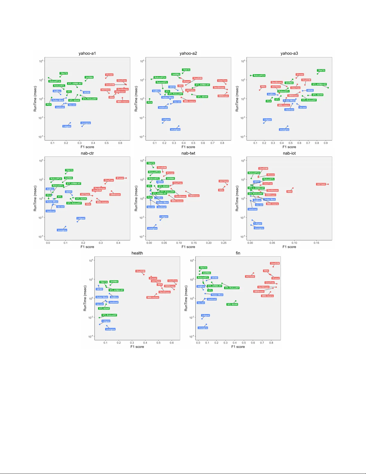
On the Runtime-Eicacy T rade-o of Anomaly Detection T echniques for Real- Time Streaming Data Dhruv Choudhary Arun Kejariwal Francois Orsini MZ Inc. ABSTRA CT Ever growing volume and velocity of data couple d with decreasing attention span of end users underscore the critical need for real-time analytics. In this regard, anomaly detection plays a key role as an application as well as a means to verify data delity . Although the subject of anomaly detection has b een researched for over 100 years in a multitude of disciplines such as, but not limited to, astronomy , statistics, manufacturing, e conometrics, marketing, most of the exist- ing techniques cannot be use d as is on real-time data streams. Further , the lack of characterization of performance – both with respect to real-timeliness and accuracy – on production data sets makes model selection very challenging. T o this end, we present an in-depth analysis, geared towards real- time streaming data, of anomaly dete ction techniques. Given the requirements with respect to real-timeliness and accuracy , the analysis presented in this pap er should ser ve as a guide for selection of the “best" anomaly detection technique. T o the best of our knowledge, this is the rst characterization of anomaly detection te chniques proposed in ver y diverse set of elds, using production data sets corresponding to a wide set of application domains. CCS CONCEPTS • Computing methodologies → Machine learning algorithms ; • Computer systems organization → Real-time systems ; KEY W ORDS Stream Mining, Anomaly Detection, Time Series, Machine Learning, Pattern Mining, Clustering 1 IN TRODUCTION Advances in technology – such as, but not limited to, decreasing form factor , network impr ovements and the growth of applications, such as location-based services, virtual reality (VR) and augmented reality ( AR) – combined with fashion to match p ersonal styles has fueled the growth of Internet of Things (Io T). Example Io T devices include smart watches, smart glasses, heads-up displays (H UDs), health and tness trackers, health monitors, wearable scanners and navigation devices, connected vehicles, drones et cetera. In a recent report [ 27 ], Cisco projected that, by 2021, there will be 929 M wearable devices globally , gr owing nearly 3 × from 325 M in 2016 at a CA GR of 23%. Permission to make digital or hard copies of part or all of this work for personal or classroom use is granted without fee provided that copies are not made or distributed for prot or commer cial advantage and that copies bear this notice and the full citation on the rst page . Copyrights for thir d-party components of this work must be honored. For all other uses, contact the owner /author(s). © 2017 Copyright held by the owner/author(s). Figure 1: Example ECG time series (10 mse c granularity) The continuous and exponential increase of volume and velocity of the data streaming from such devices limit the use of existing Big Data platforms. T o this end, recently , platforms such as Satori [ 5 ] have been launched to facilitate low-latency reactions on con- tinuously ev olving data. The other challenge in this regard pertains to analysis of real-time streaming data. The notion of real-time , though not new , is not well dened and is highly contextual [ 62 ]. The following lists the various classes of latency requirements [ 2 ] and example applications. ❚ Nano se conds : High Frequency Trading (HFT). ❚ Micro seconds : Data center applications, cloud networks. ❚ Milli seconds : T ext messaging, Publish Subscribe systems, cloud gaming. ❚ 1-3 se conds : Ad targeting. In the realm of analytics on real-time streaming data, anomaly detection plays a key r ole as an application as well as a means to verify data delity . For example, nding anomalies in one ’s vitals (see Figure 1 as an illustration) can p otentially help doctors to take appropriate action in a timely fashion, thereby potentially obviating complications. Likewise, nding anomalies in physiological signals such as electrocardiogram, electromyogram, skin conductance and respiration of a driver can help gauge the stress le vel and thereby manage non-critical in-vehicle information systems [ 49 ]. Although the subject of anomaly detection has b een researched for over 100 years [ 3 ], most of the existing te chniques cannot be used as is on real-time data str eams. This stems from a multitude of reasons – a small set of these are mentioned below . ➣ Non-conformity between the assumptions behind a given technique and the underlying distribution and/or structure of data streams ➣ The need for labels; in other words, many existing techniques are sup ervised in nature. Note that obtaining labels in a production environment is not feasible ➣ Being multi-pass and non-incremental ➣ Lack of support for recency ➣ Lack of robustness ➣ Lack of low latency computation Dhruv Choudhary Arun Kejariwal Francois Orsini Domain T echnique Summary P/N-P Inc. Robust Recency TG CF AR Statistics Mu-Sigma [ 58 , 73 , 85 , 92 , 93 , 106 , 107 ] Thresholds based on mean and standard deviation P < ✓ , ✗ > ✓ ✓ 1 µ sec Med-Mad [ 70 ] Thresholds based on median and median absolute deviation P < ✓ , ✗ > ✓ 1msec GeneralisedESD [ 42 , 43 , 86 , 98 , 102 ] Uses Student t-distribution to calculate a max number of outliers P < ✓ , ✗ > ✓ 100msec ✓ τ -Estimator [ 75 , 80 , 87 , 111 ] Measure of Spread with better Gaussian eciency than MAD P < ✓ , ✗ > ✓ 1msec Huber M-Estimator [ 54 , 105 ] Huber’s M-estimator P < ✓ , ✓ > ✓ 10msec t-digest [ 30 , 32 , 83 ] Streaming percentile based detection N-P < ✓ , ✗ > ✓ ✓ ✓ 10 µ sec ✓ AdjBox Plots [ 55 , 104 ] Adjusted whiskers for box plots N-P < ✓ , ✗ > ✓ 10msec Time Series Analysis STL [ 28 , 46 , 84 , 102 ] Seasonality Decomposition N-P < ✓ , ✗ > ✓ 100msec SARMA [ 9 , 10 , 18 , 33 , 56 ] Seasonal Auto Regr essive Moving A verage (ARMA ) P < ✓ , ✗ > 1sec STL-ARMA -KF [ 16 , 25 , 61 , 94 , 95 ] STL, ARMA on residuals P < ✓ , ✗ > 100msec STL-RobustKF [ 6 , 99 ] ARMA with Robust Kalman P < ✓ , ✗ > ✓ ✓ 100msec SDAR [ 101 , 108 , 109 ] Sequential Discounting AR P < ✓ , ✗ > ✓ ✓ 100msec RobustOutlers [ 31 , 37 , 60 , 78 ] Intervention Analysis with ARMA P < ✓ , ✗ > ✓ 10min TBA TS [ 39 , 51 , 57 , 72 , 74 ] Exponential Smoothing with Fourier T erms for Seasonality P < ✓ , ✗ > 10sec Pattern Mining HOTSAX [ 63 , 77 ] Pattern Distance based on SAX N-P < ✗ , ✓ > ✓ 1sec RRA [ 90 , 91 ] Rare Rule Anomaly based on Grammar Induction N-P < ✗ , ✓ > ✓ 1sec DenStream [ 22 ] Online Density Micro-Clustering N-P < ✓ , ✓ > ✓ ✓ ✓ 20msec CluStree [ 64 ] Hierarchical Micro-Clustering N-P < ✓ , ✓ > ✓ 100msec DBStream [ 34 , 47 , 97 , 110 ] Incremental Shared Density Based clustering N-P < ✓ , ✓ > ✓ ✓ ✓ 10msec Machine Learning MB k -means [ 13 , 113 ] Mini-batch clustering with k -means N-P < ✓ , ✓ > 10msec PCA [ 52 , 53 , 59 , 81 ] Principal Components Analysis P < ✓ , ✗ > 1msec RobustPCA [ 21 , 100 ] Low Rank Approximation P < ✓ , ✗ > ✓ 1se c IForest [ 44 , 71 , 96 ] Isolation Forests N-P < ✓ , ✓ > 100msec OneSVM [ 12 , 89 ] One Label SVM P < ✗ , ✓ > 1sec T able 1: Classication of anomaly detection techniques. P: Parametric technique, N-P: Non-parametric technique, Pt: Point anomalies, Pa: Pattern anomalies, Inc.: Incremental technique, Robust: Robustness to noise, Re cency: Ability to weigh obser- vations by age, TG: Time Granularity of a data stream that can use the method, CF AR: Constant False Alarm Rate. ➣ Lack of support for constant false alarm rate ➣ Lack of scalability Further , other characteristics of Io T devices such as, but not limited to, small storage, small power budgets consumption et cetera limit the use of o-the-shelf anomaly detection te chniques. Last but not least, constantly e volving nature of data streams in the wild call for support for continuous learning. As overviewed in [ 3 ], anomaly detection has been researched in a wide variety of disciplines, for example, but not limited to, operations, computer vision, networking, marketing, and so cial media. Unfortunately , there does not exist a characterization of the performance of anomaly detection techniques – b oth with respect to real-timeliness and accuracy – on pr oduction data sets. This in turn makes model selection very challenging. T o this end, in this paper , we pr esent an in-depth analysis, geared towar ds real-time streaming data, of a large suite of anomaly detection techniques. In particular , the main contributions of the pap er are as follows: ❏ W e present a classication of ov er 20 (!) anomaly detection techniques across seven dimensions (refer to T able 1 ). ❏ As a rst, using over 25 (!) real-world data sets and real har d- ware, we present a detailed evaluation of the real-timeliness of the anomaly dete ction techniques listed in Table 1 . It is important to note that the evaluation was carried out in an unsupervise d setting. In other words, irr espective of the availability of labels, a model was not trained a priori. ❏ W e present detailed insights into the p erformance – as mea- sured by precision, recall and F 1 score – of the anomaly detec- tion techniques listed in T able 1 . Specically , w e also present a deep dive view into the behavior subject to the following: ❚ Tr end and level shifts ❚ Change in variance ❚ Change in seasonal level ❚ Change in seasonality period ❏ W e present a map of the accuracy-runtime trade-o for the anomaly detection techniques. ❏ Given an application domain and latency requirement, based on empirical evaluation, we make recommendations for the “best" technique for anomaly detection. Given the requirements with respect to real-timeliness and accuracy , we believe that the analysis presented in this paper should serve as a guide for selection of the “best" anomaly detection te chnique. T o the best of our knowledge, this is the rst characterization of anomaly dete ction techniques proposed in a ver y diverse set of elds (refer to T able 1 ) using production data sets corr esponding to a wide set of applications. The rest of the paper is organized as follows: In Section 2 , we dene the terms in the subse quent sections. Section 3 present a brief overview of the techniques listed in T able 1 . Section 4 details the experimental set up and Section 5 walks the reader through a deep div e of the analysis and insights learned from the experiments. Finally , in Se ction 6 we conclude with directions for future w ork. 2 PRELIMINARIES In this section we dene the terms used in the rest of paper . Denition 2.1. Point Anomalies: are data points which deviate so much from other data points so as to arouse suspicions that it was generated by a dierent mechanism [ 48 ]. Denition 2.2. Pattern A nomalies: Continuous set of data p oints that are collectively anomalous even though the individual points may or may not be point anomalies. Denition 2.3. Change Detection: This corresponds to a perma- nent change in the structure of a time series, e.g., change in the mean level ( Level Shift ), change in the amplitude of seasonality ( Seasonal Level Shift ) or change in the noise amplitude ( V ariance Change ). On the Runtime-Eicacy Trade-o of Anomaly Detection T echniques for Real- Time Streaming Data Denition 2.4. Concept Drift: This corresponds to the change in statistical properties, for example, the underlying distribution, of a time series over time. Next, we dene the desirable properites for anomaly detection techniques geared towards real-time data streams. Property 2.1. Incremental: A property via which a technique can analyze a new data p oint without re-training a model. Property 2.2. Recency: Under this, a technique assigns weights to data points which decays with their age. In other words, recent data points play a dominant role during model training. Property 2.3. Constant False Alarm Rate (CF AR): A property under which the upper limit on the false alarm rate (F AR) – dened as the ratio of falsely tagged anomalies and the total numb er of non- anomalous p oints – is constant. 3 BA CK GROUND As mentioned earlier in Section 1 , the subject of anomaly detection has been researched for over 100 years [ 3 ]. A detailed walkthrough of prior work is beyond the scope of this paper (the reader is referred to the b ooks [ 7 , 14 , 48 , 88 ] or sur veys [ 17 , 24 , 26 , 40 , 45 , 79 , 114 ] written on the subject). In the se ction, we present a brief overview of the techniques listed in T able 1 . 3.1 Statistics In this subsection we briey overview the common statistical te ch- niques used for anomaly detection. 3.1.1 Parametric A pproaches. One of the most commonly used rule to detect anomalies – popularly referred to as the µ ± 3 • σ rule – whereby , observations that lie 3 or more deviations ( σ ) away from the mean ( µ ) are classied as anomalies. The rule is based on the following two assumptions: ( a) the underlying data distribution is normal and (b) the time series is stationar y . In practice, production time series often do not satisfy the ab ove, which results in false positives. Further , both µ and σ are not robust against the presence of anomalies. T o this end, several robust estimators have b een proposed. Specically , Huber M-estimator [ 54 ] is commonly used as a robust estimate of location, whereas median, τ estimator [ 111 ] and Median Absolute Deviation (MAD) are commonly used as robust estimates of scatter . In the presence of heavy tails in the data, t -distribution [ 112 ] is often used as an alternative to the normal distribution. The Gen- eralized Extreme Studentized Deviate (ESD) test [ 86 ] uses the t - distribution to detect outliers in a sample , by carrying out hypothe- sis tests iteratively . GESD requires an upp er bound on the numb er of anomalies, which helps to contain the false alarm rate (F AR). 3.1.2 Non-parametric A pproaches. It is routine to observe pro- duction data to exhibit, for example but not limited to, skewed and multi-modal distribution. For nding anomalies in such cases, several non-parametric appr oaches have been proposed over the years. For instance, t -digest [ 32 ] builds an empirical cumulative density function (CDF), using adaptive bin sizes, in a streaming fashion. Maximum bin size is determined base d on the quantile of the value max ( 1 , ⌊ 4 N δ q ( 1 − q )⌋ ) , where q is the quantile and δ is a compression factor that controls the space requirements. In a similar vein, adjusted Boxplots [ 104 ] have been proposed to identify anomalies in ske wed distributions. For this, it uses a robust measure of the skew called medcouple[ 19 ]. 3.2 Time Series Analysis Observations in a data streams exhibit autocorrelation. Thus, prior to applying any anomaly detection technique, it is critical to weed out the autocorrelation. A uto Regressive Moving A verage (ARMA ) [ 18 ] models have been commonly used for analysis of stationary time series. ARMA models are formulated as State Space Models (SSM) [ 33 ], where one can employ K alman Filters for model estima- tion and inference. K alman lters (KF) [ 61 ] are rst order Gaussian Markov Processes that provide fast and optimal inference for SSMs. KFs assume that the hidden and observed states are Gaussian pro- cesses. When that assumption fails, the estimates obtained via KFs can p otentially b e biase d. Robust Kalman Filters ( RobustKF ) [ 99 ] treat the residual err or as a statistical property of the process and down weight the impact of anomalies on the observed and hidden states. Sequential Discounting AutoRegressive (SDAR) lters assign more weight to recent obser vations in order to adapt to non-stationar y time series or change in dynamics of a system [ 108 ]. Further , a key feature of SDAR lters is that they update incrementally . A dis- count rate is specied to guide the rate of adaptation to changing dynamics. 3.3 Pattern Mining Time series with irregular but self-similar patterns are dicult to model with parametric methods. Non-parametric data mining ap- proaches that nd anomalous patterns and/or subsequences have been proposed for such time series. SAX is a discretization tech- nique that transforms a series from real valued domain to a string dened over a nite alphab et F of size a [ 63 ]. It divides the real num- ber scale into equal probabilistic bins based on the normal model and assigns a unique letter from F to every bin. Before discretiza- tion, SAX z-normalizes the time series to map it to a probabilistic scale. It then forms w ords from consecutive observations that fall into a sliding window . The time series can now be represented as a do cument of words. SAX employs a dimensionality reduction technique called Pie cewise Aggregate Appr oximation (P AA) which chunks the time series into equal parts and computes the average for each part. The reduced series is then discretized for further processing. The key advantage of SAX o ver other discretization heuristics [ 20 , 38 ] is that the distance b etween two subsequences in SAX low er bounds the distance measure on the original series. This allows SAX to be used in distance based anomaly dete ction te chniques. For example, HOTSAX [ 63 ] uses SAX to nd the top- k discords. Another method that leverages SAX is the Rare Rule Anomaly (RRA) technique [ 90 ]. RRA induces a context fr ee grammar from the data. The grammar induction process compresses the input sequence by learning hierarchical grammar rules. The inability of compressing a subse quence is indicative of the Kolmogoro v randomness of the sequence and hence, can be treated as b eing an anomaly . RRA uses the distance to the closest non-self match subsequence as the anomaly score. 3.4 Machine Learning Machine Learning approaches such as clustering, random for ests, and deep learning are ver y eective in modeling complex time Dhruv Choudhary Arun Kejariwal Francois Orsini series patterns. Having said that, the training time is usually v ery high and many of these techniques are not incr emental in nature. Thus, most of these techniques work in batch mode where training is performed perio dically . Isolation forests [ 71 ] is a tree base d technique that randomly splits the data recursively in an attempt to isolate all observations into separate leafs. The numb er of splits ne eded to reach a data p oint from the root no de is called the path length. Many such random split forests are constructe d and the average path length to r each a point is used to compute the anomaly score . Anomalous observations are closer to the root node and hence have lower average path lengths. One Label Support V ector Machines (SVMs) [ 89 ] are often used to construct a non-linear decision boundar y around the normal instances, thereby isolating anomalous observation that lie away form the dense regions of the support vectors. A key advantage of this technique is that it can be used even with small number of data points, but are potentially slow to train. Clustering There are two main approaches to handle the stream clustering problem: Micro-Clustering ( MC ) and Mini-Batching ( M B ). Micro-Clustering A large number of techniques follow a 2-phase Micro-clustering approach [ 8 ] which has b oth an online as well as an oine com- ponent. The online component is a dimensionality reduction step that computes the summary statistics for observations v ery close to each other (called micro-clusters). The oine phase is a traditional clustering technique that ingests a set of MC s to output the nal clustering, which can be used to identify anomalous MC s. DenStream is a density-based streaming te chnique which uses the MC paradigm [ 22 ]. In the online phase , it creates two kinds of MC s: potential micro-clusters ( p M C ) and anomalous micro-clusters( o M C ). Each cluster maintains a weight w which is an exponential function of the age of the observations in the cluster . w is updated period- ically for all clusters to reect the aging of the observations. If w is above a threshold ( t α ), it is deemed as a core micro-cluster . If w is more than β t α (where 0 < β < 1 ), the cluster is de emed as a p M C , otherwise it is deemed a o M C . When a new observation arrives, the technique looks for a p M C that can absorb it. If no p M C is found, it looks for an o M C that can absorb the observation. If no o M C is found, a new o M C is instantiated. Older clusters are perio dically removed as their w be come smaller . DBStream is an incremental clustering technique that decays MC s, akin to DenStream . It also keeps track of the shar ed density between MC s. During the oine phase, it leverages this shared density for a DBSCAN-style clustering to identify anomalous MC s. Hierarchical clustering techniques such as Clustree use the MC paradigm to construct a hierarchical height balanced tree of MC s [ 64 ]. MC corresponding to an inner node is an aggregation of the clusters of all its children. A key advantage of these techniques is their being incremental; having said that, the data structures can grow balloon in size. For anomaly detection, the distance of a new observation from the closest leaf MC is used as the anomaly score. Mini-Batching The second approach for a data stream clustering entails batch clus- tering of a sample generated from the data stream. These samples are signicantly larger than the micro-clusters and hence the name mini-batch. An example te chnique of this kind is the mini-batch k -means which uses cluster centroids from the previous clustering step to reduce the convergence time signicantly [ 35 ] . 3.5 Potpourri Seasonality in time series is commonly observed in production data. Filtering of the seasonal component is critical for eectiv e anomaly detection. In this regard, a key challenge is how to determine the the seasonal period. For this, a widely used approach is to detect strong peaks in the auto-correlation function coupled with statistical tests for the strength of the seasonality . Seasonal- T rend-Loess ( STL ) [ 28 ] is one the most commonly used techniques for removing the seasonal and trend components. STL uses LOESS [ 29 ] to smooth the seasonal and trend comp onents. Presence of anomalies can potentially induce distortions in trend which in turn can result in false positives. T o alleviate this, Robust STL iteratively estimates the weights of the residual – the number of robustness iterations is an input manual parameter . The downside of this is that the r obustness iterations slow do wn the run time per- formance. V allis et al. [ 103 ] proposed the use of pie cewise medians of the trend or quantile regression – this is signicantly faster than using the robustness iterations. Although STL is ee ctive when seasonality is xed over time, moderate changes to seasonality can be handled by choosing a lower value for the “s.window" parameter in the STL implementation of R . Seasonal ARMA ( SARMA ) models handle seasonality via the use of seasonal lag terms [ 33 ]. A key advantage with the use of SARMA models is the supp ort for change in seasonality parameters over time. However , SARMA is not robust to anomalies. This can b e addressed via the use of robust lters [ 23 ]. Note that the estimation of extra parameters increases the relative model estimation time considerably . SARMA models can also handle multiple seasonalities at the expense of complexity and runtime. Akin to SARMA, TBA TS is an exponential smoothing model which handles seasonality using Fourier impulse terms [ 72 ]. Principal Components Analysis (PCA) is another common method used to extract seasonality . However , the use of PCA requires the data to b e represented as a matrix. One way to achieve this is to fold a time series along its seasonal boundaries so as to build a rectangular matrix ( M ) where each row is a complete season. Note that PCA is not robust to anomalies as it uses the covariance matrix which is non-robust measure of scatter . T o alleviate this, Candes et al. proposed Robust PCA ( RPCA ) [ 21 ], by decomposing the matrix M into a low rank comp onent( L ) and a sparse component( S ) by minimizing the nuclear-norm of M . 4 EXPERIMEN T AL SET UP In this section, we detail the data sets used for evaluation, the underlying methodology and walk through any transformation and/or tuning needed to ensure a fair comparative analysis. 4.1 Data Sets T able 2 details the data sets used for evaluation. Note that the data sets belong to a diverse set of domains. The diversity of the data sets is reected based on the following attributes: ❚ Seasonality Period (SP): Most of these time series exhibit seasonal b ehavior and the SP increases with TG . For instance, the minutely time series of operations data experience daily On the Runtime-Eicacy Trade-o of Anomaly Detection T echniques for Real- Time Streaming Data Domain Description Acronym Len WinSize PL Cnt TG Lab els SP SJ LS VC SLD SLS NAB [ 67 ] NAB Advertising Click Rates nab-ctr 1600 240 20 4 1 hr ✓ 24 ✓ ✓ ✓ NAB T weet V olumes nab-twt 15800 2880 20 4 1 hr ✓ 288 NAB Ambient T emperature nab-iot 7268, 22696 5000 20 1 1 hr ✓ 24 ✓ ✓ ✓ ✓ Y AD [ 66 ] Real operations series yahoo-a1 1440 720 10 67 1hr ✓ 24,168 ✓ ✓ ✓ Synthetic operations series yahoo-a2 1440 720 10 100 1hr ✓ 100-300 ✓ ✓ ✓ Synthetic operations series yahoo-a3 1680 720 10 100 1hr ✓ 24,168 ✓ ✓ ✓ HFT [ 4 ] Facebook Trades Dec. 2016 n-fb 334783 10000 60 1 1 se c Manual ✓ ✓ Google Trades Dec. 2016 n-goog 127848 10000 60 1 1 sec Manual ✓ ✓ Netix Trades Dec. 2016 n-nx 177018 10000 60 1 1 sec Manual ✓ ✓ SPY Trades Dec. 2016 n-spy 392974 10000 60 1 1 sec Manual ✓ ✓ Ops. Minutely Operations Data ops-* 120000 14400 60 44 1 min 1440,60 ✓ ✓ ✓ ✓ Io T [ 15 ] Power Usage of Freezer iot-freezer01 432000 23820 1800 1 1 sec 2382 2370-2390 ✓ ✓ Power Usage of Fridge iot-fridge01 432000 81900 1800 1 1 sec 8190 7900-8200 ✓ ✓ Power Usage of Dishwasher iot-dishwasher01 432000 20000 1800 1 1 sec ✓ ✓ Power Usage of Freezer iot-freezer02 432000 20000 1800 1 1 sec ✓ ✓ Power Usage of Fridge iot-fridge02 432000 30360 1800 1 1 sec 3036 3030-3080 ✓ ✓ Power Usage of Lamp iot-lamp02 432001 20000 1800 1 1 sec 2370-2390 ✓ ✓ Power Usage of Freezer iot-freezer04 432000 41500 1800 1 1 sec 4150 4100-4200 ✓ ✓ Power Usage of Fountain iot-fountain05 432000 432000 1800 1 1 sec 86400 ✓ ✓ Power Usage of Fridge iot-fridge05 432000 47500 1800 1 1 sec 4750 4720-5000 ✓ ✓ Health [ 41 ] ECG Sleep Apnea [ 82 ] health-apnea-ecg/a02 15000 2000 40 1 10 msec ✓ 100 90-110 ✓ ECG Seizure Epilepsy [ 11 ] health-szdb/sz04 10000 2000 40 1 5 msec ✓ 200 190-230 ✓ ECG Smart Health Monitoring [ 76 ] health-shareedb/02019 15000 2000 40 1 8 msec ✓ 110 95-105 ✓ Skin Resistance Under Driving Stress [ 50 ] health-drivedb/driver02 22000 2000 40 1 60 msec ✓ ✓ Skin Resistance Under Driving Stress [ 50 ] health-drivedb/driver09/foot 20000 2000 40 1 60 msec ✓ ✓ Respiration Under Driving Stress [ 50 ] health-drivedb/driver09/resp 20000 2000 40 1 60 msec ✓ ✓ ECG Premature V entricular Contraction [ 65 ] health-qtdb/0606 10000 2000 40 1 4 msec ✓ 176 170-180 ✓ T able 2: Anomaly detection datasets. Len: A verage length of the time series, WinSize: Window Size, PL: Pattern Length, Cnt: Number of Series, TG: Time Granularity , SP: Seasonal Perio d, SJ: Seasonal p eriod Jitter , LS: Level Shift, VC: V ariance Change, SLD: Seasonal Level Drift, SLS: Seasonal Level Shift Figure 2: Illustration of the characteristics of data sets from dierent domains seasonality (p eriod= 1440 ). In contrast, secondly time series of Io T workloads experience v ery long seasonalities (period= 2 k - 90 k ) depending on the operation cycles of the appliances. Health series have coarse TG but the seasonal p eriodicity are usually small(period= 100 - 200 ). ❚ Seasonal Jitter : It refers to the presence of jitter in seasonal periods, and is an artifact of coarse TG . Io T and Health time series exhibit this property . ❚ Non-stationarity : Time series e xhibit one or more types of nonstationarities with respect to their level (amplitude) and variance. Figure 2 illustrates characteristics of these time series. From the gure we note that most of the series are non-stationary and e xhibit one of these types of nonstationarities: The Numenta Anomaly Benchmark (NAB) [ 67 ] and the Y ahoo A nom- aly Dataset (Y AD) [ 66 ] – which are considered industry standard – provide labels. NAB itself is a collection of time series from multiple domains like Advertising Click Through Rates ( nab-ctr ), volume of tweets per hour ( nab-twt ), sensor data for temp erature ( nab-iot ). The NAB series used herein have hourly granularity . Y AD is com- posed of three distinct data sets: yahoo-a1 comprises of a set of operations time series with hourly granularity , whereas yahoo-a2 and yahoo-a3 are synthetic time series. Anomalies dete ction in the context of high frequency trading (HFT) surfaces arbitrage opportunities and hence can have poten- tially large impact to the bottom line. In light of this, w e included a month long time series of trades for the tickers FB , GOOG , NFLX and SPY . The time series, purchased fr om QuantQuote [ 4 ], are of secondly granularity . W e collected 44 minutely time series of operations data from our production environment. The ECO dataset [ 15 ] comprises of secondly time series of power usage. Given the increasing emphasis Dhruv Choudhary Arun Kejariwal Francois Orsini on healthcare apps owing to the use Io T devices in Healthcare domain, we included seven data sets from Physiobank [ 41 ]. 4.2 Methodology T o emulate unbounded evolutionary data streams, we chose long time series and applied anomaly detection techniques for every new data point in a str eaming fashion. Further , we limit the number of data points a technique can use to determine whether the most recent observation is anomalous. A common way of doing this is to dene a maximum Window Size that can be used for training or modeling. Window size is an imp ortant hyper-parameter which has a dir ect correlation with runtime and accuracy . Longer windows require more processing time, while shorter windows result in drop in accuracy . For a fair comparative analysis, we set an upp er limit on the values of windo w size for dierent data sets, as listed in T able 2 . The values were set based on the data set, e.g., for the minutely operations time series (seasonal period=1440), one would need at least 10 periods [ 68 ] to capture the variance in the seasonal patterns, giving a seasonal p eriod of 14400 . This is the maximum allowed valuer; techniques may choose a shorter seasonal period depending on their requirements. For instance, TBA TS needs fewer number of periods to learn and hence, we used only 5 p eriods (WinSize= 7200 ) in the experiments. Data sets such as Y AD have xed seasonal periods due to hourly TG , and hence, require much smaller window sizes to achieve maximum accuracy . Io T data sets have the longest window sizes due to the long seasonal periods. Pattern Length (PL) is a hyper-parameter of all pattern mining techniques. The value of PL is dependent on the application and the typ e of anomalies. For example, IoT workloads require a PL of ≈ 30 minutes, whereas Health time series usually require a PL of only 40 . A moving window equal to the PL is used to extract subsequences from the time series. Although pattern anomalies are typically not of xed length in production data, most techniques require a xed length to transform the series into subsequences. T o alleviate this, post-processing can be used to string together multiple length anomalies [ 90 ]. In order to characterize the runtime p erformance of the tech- nique listed in T able 1 , we measured the runtime needed to process every ne w point in a time series. For ev ery new data point in a time series, each technique was run 10 times and the me dian runtime was recorded. Across a single time series, the run-times for all the data points in the time series were averaged. Across multiple time series in a group, geometric mean of the run-times 1 of the individ- ual series is used to r epresent the runtime for the group. Given that some of the data sets listed in T able 2 have short time series ( e.g., NAB and Y AD ), we replicate these series 10 times to increase their length. All run-times are reported in milliseconds (msec). 4.2.1 Metrics. Accuracy for labeled data sets is calculate d in terms of the correctly identie d anomalies calle d True Positives (TP), falsely detected anomalies called False Positives (FP) and missed anomalies called False Negatives (FN). T o measure accuracy of a single time series, we use the following three metrics: 1 This approach is an industry standard as evidenced by its use by SPEC [ 1 ] for over 20 years. ❏ Precision: dened as the ratio of true positives (TP) to the total detected anomalies: P r = T P T P + F P ❏ Recall: dened as the ratio of true positives (TP) to the total labeled anomalies: Re = T P T P + F N ❏ F 1 -score: dened as the weighted harmonic mean of Preci- sion and Re call: F 1 = ( 1 + β 2 ) P r ∗ R e β 2 ∗ P r + R e , where β is a constant that weights precision vs recall based on the application In most applications, it is common to set β =1, giving equal weight- age to precision and recall. But for healthcare, r ecall is sometimes more important than precision and hence β =2 is often used [ 69 ]. This is b ecause false negatives can b e catastrophic. T o calculate accuracy acr oss a group of time series, we report the micr o-average F 1 -score [ 36 ], which calculates precision and recall across the whole group. The use of this is subject to time series in a group being similar to each other . Most of our data sets are labeled with point anomalies. In light of this, we propose the following metho dology to compute accu- racy for detecte d patterns against labeled point anomalies. Let ( Y 1 , Y 2 , Y 3 , . . . Y p , Y p + 1 ) denote a time series and the pattern Y 2 - Y p be detected as a pattern anomaly . Let Y p − 1 be a true anomaly . A naive way to compute a T P is to have a pattern anomaly end at the true anomaly . In this case, Y 2 - Y p would be considered a F P . In contrast, T P can correspond to an instance where a true anomaly occurs anywhere inside the boundary of an anomalous pattern. Pattern anomalies are very often closely spaced due to the prop- erty of neighb orhood similarity as described by Handschin and Mayne [ 63 ]. Given this, it is important to count each true anomaly only once even if multiple overlapping pattern anomalies ar e de- tected. A p ost-processing pass can help weed out such overlapping subsequences. Given that the methodology of calculating accuracy is so dier- ent for pattern techniques, we advise the r eader to only compare accuracies of pattern techniques with other pattern techniques. 4.2.2 System Configuration. T able 3 details the hardware and software system conguration. T able 4 details the R and P y t h on packages used. For HOTSAX and RRA , we modie d the implemen- tation so as to make them amenable to a str eaming data context. Architecture Intel(R) Xeon(R) Frequency 2.40GHz Num Cores 24 Memory 128GB L1d cache 32K L1i cache 32K L2 cache 256K L3 cache 15360K OS V ersion CentOS Linux release 7.1.1503 R, Python 3.2.4, 2.7 T able 3: System Conguration R stream , streamMO A MASS rrcov jmotif robustbase forecast tsoutliers rpca Python pykalman scikit-learn tdigest statsmodels T able 4: Packages and Libraries On the Runtime-Eicacy Trade-o of Anomaly Detection T echniques for Real- Time Streaming Data 4.3 Hyper-parameters In the interest of r eproducibility , we detail the hyper-parameters used for the techniques liste d in T able 1 . In addition, we detail any transformation and/or tuning needed to ensure a fair comparative analysis. 4.3.1 Statistical te chniques. For parametric statistical te chniques such as mu-sigma , med-mad et cetera, we set the threshold to 3 • σ or its equivalent robust estimate of scale. A constant false alarm rate can be set for te chniques such as t-digest and GESD . In case of the former , we set the threshold at 99 . 73 th percentile which is equivalent to 3 • σ . In case of the latter , one can set an upper limit on the number of anomalies. Based on our experiments, w e set this parameter to 0 . 02 for all, but the Health data sets. The parameter was set to 0 . 04 for the the Health data sets to improve r ecall at the expense of precision. Model parameter estimates are computed at each new time step over the mo ving window . As these techniques do not handle sea- sonality or trend, we removed seasonality and trend using STL and evaluate these techniques on the residual of the STL. In light of this, i.e., statistical techniques are not applicable to the raw time series in the presence of seasonality or trend, the accuracy of these techniques should not be compared with ML and Pattern Mining based techniques. 4.3.2 Time series analysis te chniques. Parametric time series analysis techniques such as TBA TS , SARMA , STL- ARMA estimate model parameters and evaluate incoming data against the model. Retraining at every time step is often unnecessar y as the temporal dynamics do not change at every point. In practice , it is common to retrain the model periodically and this retraining perio d is another hyper-parameter . This period dep ends on the application, but it should not be greater than the window size. W e set the retraining period to be the same as the window size. W e include the training runtime as part of the total runtime of a techniques so as to assess the total detection time for anomalies. STL with default parameters assumes periodic series. T o allow gradual seasonal level drift, we set the stl-periodic parameter equal to 21 . For RobustSTL , we use 4 robust iterations. SD AR is an incre- mental technique that requires a learning rate parameter ( r ). Based on our experiments, we set r = 0 . 0001 . RobustKF is the robust kalman lter by Ting et al.[ 99 ] which requires parameters α and β for the G a mma prior on the robustness weights. W e set α = β = 1 . W e also evaluate te chniques based on Inter vention A nalysis of time series implemented in the tsoutliers package of R . These tech- niques are signicantly slow er than most other techniques we eval- uate in this work, e.g., for a series with 2 k data points, it took over 5 minutes (!) for parameter estimation. Clearly , these techniques are non-viable for real-time streaming data. 4.3.3 Paern mining and machine learning techniques. Most pat- tern techniques require pattern length (PL) as an input parameter . T able 5 lists the specic parameters and their respective values for each technique. HOTSAX and RRA are robust to presence of trend in a time series as they use symb olic approximation, but they do require the series to b e studentized. All the other pattern techniques are not robust to presence of trend as the y use the underlying real valued series directly . Thus, all the subse quences need to be mean adjusted (i.e., subtract the mean from all the data points) to av oid spurious anomalies due to changing trend. Scale normalization is not carried as change in scale is an anomaly itself. Keogh et al. pr oposed a noise reduction technique wherein a subse- quence is rejected if its variance lies b elow a threshold, ϵ [ 63 ]. Our experiments show that this preprocessing step is critical, fr om an accuracy standpoint, for all pattern mining techniques considerably . Therefore, we use it by default, with ϵ = 0 . 01 . DenStream is the only T echnique Parameters Description HOTSAX paa-size= 4 , a-size= 5 P AA Size, Alphabet Size RRA paa-size= 4 , a-size= 5 P AA Size, Alphabet Size DenStream epsilon= 0 . 9 lambda= 0 . 01 MC radius, Decay Constant DBStream r= 0 . 5 , Cm= 5 , shared-density=True MC radius, minimum weight for MC ClustTree max-height= 5 , lambda= 0 . 02 Tr ee Height, Decay Constant DBScan eps= . 05 Threshold used to re-cluster ClusTree IForest n-estimators= 50 , contamin.= . 05 Number of Trees, Number of Outliers OneSVM nu= 0 . 5 , gamma= 0 . 1 support vectors, kernel coe. MB k -means n-clusters= 10 , batch-size= 200 Number of Clusters, Batch Size T able 5: Parameters for Pattern Mining and Machine Learn- ing T echniques MC technique that works without an explicit re-clustering step. The technique can classify outlier micro-clusters ( oM C ) as anoma- lous, but this leads to a higher false positive rate. Alternatively , one can take the distance of the points to the near est p M C as the strength of the anomaly . This makes DenStream less sensitive to the MC radius ϵ as well. DenStream and DBStream are incremental techniques. Hence , they do not nee d an explicit windo w size param- eter; having said that, the y use a decay constant λ to discount older samples. IForest and OneSVM are not incremental techniques and hence, need to be retrained for each time step . MBKmeans is also not incremental, how ever , it uses cluster centroids from pr evious run to calculate the new clusters, which allows the clustering to converge faster . 5 ANAL YSIS In this se ction we present a de ep dive analysis of the techniques listed in T able 1 , using the data sets detailed in T able 2 . 5.1 Handling Non-stationarity In this subsection we walk the reader through how the dierent techniques handle the dierent sources of non-stationarity e xhib- ited by the data. Most techniques assume that the underlying pro- cess is stationary or evolving gradually . However , in practice, this assumption does not hold true thereby resulting in a larger number of false positives immediately after a process change. Though de- tecting the change is itself important, the false positives adversely impact the ecacy in a material fashion. ❐ Tr end and Level Shifts (LS): Statistical techniques are not robust to trend or level shifts. Consequently , their perfor- mance is dependent on the window size, which decides how fast these techniques adapt to a new level. Time series anal- ysis techniques base d on state space mo dels (e.g., SARMA , TBA TS ) can identify level shifts and adapt to the new level without adding false positives. Figure 3a illustrates a nan- cial time series, where SARMA and SDAR detect the level shift as an anomaly . me d-mad can also dete ct the level shift but it surfaces many false p ositives right after the level shift. Pattern techniques mean-adjust the patterns. Hence, in the Dhruv Choudhary Arun Kejariwal Francois Orsini (a) An illustration of a Level Shift (b) An example illustrating adaptation of SDAR to change in variance (c) Illustration of Seasonal Level Shift Figure 3: Impact of Non-Stationarities presence of level shifts, they do not surface false positives as long as the pattern shapes do not change rapidly . ❐ V ariance Change (VC): Figure 3b shows an operations se- ries with a variance change. Iterative techniques such as STL-SD AR adapt faster to changing variance which allows them to limit the numb er of false positives. On the other hand, STL-ARMA and SARMA are periodically re-trained and oscillate around the true error variance. ❐ Seasonal Drift (SD) : Gradually changing seasonal pattern is often observed in iot and ops time series. SARMA adapts to such a drift with default parameters. STL adapts as well if the pe r iod i c parameter is set to false – this ensures that seasonality is not averaged out across seasons. ❐ Seasonal Level Shift (SLS) : SLS is again e xhibited predom- inantly in iot and ops series as illustrated in Figure 3c . TBA TS does not adapt to SLS or SD as it handles seasonality using Fourier terms and assumes that the amplitudes of seasonal- ity do not change with time. SARMA handles SLS smo othly as it runs a Kalman-Filter on the seasonal lags and hence only detects anomalies when the shift happens. On the other hand, STL is not robust to SLS and may result in false posi- tives as exemplied by Figure 3c . Pattern T echniques such as DBStream are very robust to SLS and can dete ct the pattern around the shift without any false positives. ❐ Seasonal Jitter (SJ) : SJ is an artifact of ne-grain TG and is predominantly exhibited in iot (sec) and health (msec) time series. Statistical and time series analysis techniques do not model this non-stationar y behavior . As a consequence, in such cases, only pattern anomaly techniques can be used. 5.2 Runtime Analysis In this section we present a characterization of the techniques listed in T able 1 with respect to their runtimes. In the gures referenced later in the section, the b enchmarks are organized in an increasing order of seasonal period from left to right. ❐ Statistical techniques: From Figure 4a we note that mu- sigma and t-digest – recall that these are incr emental too – are the fastest( <10 µ s e c ) in this category . Robust techniques are at least an order of magnitude slower! This stem from the fact that these techniques solv e an optimization problem. Although GESD is the slowest technique in this category , it let’s one set an upper bound on the numb er of anomalies, which in turn helps control the false alarm rate(CF AR). ❐ Time series analysis techniques: From Figure 4b we note that STL is the fastest technique (1-5 mse c ) in this category . Having said that, the runtime increases considerably as the seasonal period increases (left to right). Robust STL is an order of magnitude slower than STL even when the number of robust iterations is limited to 4 . This can be ascribed to the fact that iterations with the robust weights in STL are signicantly slower than the rst one. SARMA and TBA TS are signicantly slower than most other techniques in this categor y . This is an artifact of the win- dow length needed to t these mo dels being proportional to the seasonal period and thus, model parameters need to be estimated on a much larger window . On the other hand, a technique such as STL-ARMA applies ARMA on the residual of STL and therefore does not ne ed to deal with seasonality , which allows for a much smaller training windo w . Runtimes for TBA TS, SARMA and RPCA increase exponentially with an increase in seasonal period. Hence, for secondly time series, these methods become nonviable. SD AR and RobustKF are fast incremental te chniques that can execute in µ s e c s . Howev er , these techniques cannot b e applied to seasonal series as is. This limitation can b e allevi- ated by applying STL as a preprocessing step. From Figure 4b , we note that STL-SDAR and STL-RobustKF are almost as fast as STL. Even though STL- ARMA trains on small training windows, note that it adds signicant additional runtime to STL . This impact is not as pr ominent in the case of the ops and n data sets - this is due to the fact that STL itself has On the Runtime-Eicacy Trade-o of Anomaly Detection T echniques for Real- Time Streaming Data (a) Statistical te chniques (b) Time series analysis techniques (c) Pattern and machine learning techniques Figure 4: Runtime characterization of anomaly detection techniques long runtimes for these data sets. Although we note that PCA is a very fast technique, its accuracy is v ery low (this is discussed further in the next subsection). This is owing to the PCs being not robust to anomalies. themselves. ❐ Pattern and machine learning techniques: From Fig- ure 4c we note that IForest and OneSVM have the worst runtime performance as they are not incr emental and they need to be traine d for every new data point. MB-Kmeans is relatively faster even though it performs clustering for every new point. This is because the clustering has fast conver- gence if the underlying model drift is gradual. Although the internal data structures HOTSAX and RRA can be generated incrementally , nding the farthest point using these structures accounts for majority of the runtime. Thus, the runtime for HOTSAX, RRA is not dependent on the window size; instead, it is a function of the variance in the data. Data sets such as n , ops and iot exhibit high variance due to ne grain TG – this impacts the runtime of HOTSAX, RRA . med data set on the other hand has coarse TG and therefore have a lo w variance in terms of the shapes of patterns and hence, HOTSAX and RRA are signicantly faster for them. DBStream is the fastest micro-clustering technique across all data sets even though it does hav e an oine clustering component which is executed for every new point. This is because it maintains the shared density b etween MC s on-the- y and then uses DBScan over these MC s to produce the nal clustering. DenStream is slower than DBStream b ecause the distance of a data point to all p M C ’s needs to be computed to calculate the strength of the anomaly . Alternatively , one can tag all oM C s as anomalous which helps to reduce runtime but adversely impacts the F AR. From Figure 4c we note that ClusTr ee is the slowest of all the micro-clustering te chniques. Figure 5: Illustration of the impact of lack of robustness 5.3 Accuracy-Speed Tradeo Figure 6 charts the landscape of accuracy-sp eed tradeo for the techniques listed in Table 1 across all data sets tabulated in T able 2 . T able 6 details the Precision , Recall along with the F 1 -score . In this rest of this subsection, we present an in-depth analysis of the trade- o from multiple standpoints. ❐ Robustness and False Positives: T echniques such as me d- mad surface a higher numb er of anomalies, which improves recall at the e xpense of precision as evident from T able 6 . For best accuracy , we recommend to use robust techniques with CF AR such as GESD . From Table 6 we note that GESD outper- forms most other statistical techniques. On the other hand, from Figure 6 we note that GESD has the highest runtime amongst the statistical techniques. ❐ Model Building: Estimating model parameters in the pres- ence of anomalies can potentially impact accuracy adv ersely if the technique is not robust. This is observed from Fig- ure 5 wherein an e xtreme anomaly biases the model obtained Dhruv Choudhary Arun Kejariwal Francois Orsini Figure 6: Landscape of accuracy-spe ed tradeo. Note that Y -axis is on log scale. For ease of visual analysis, the range for X-axis is custom for each dataset. T echniques are grouped according to scale - Blue: Statistical, Green: Time Series, Red: Pattern via SARMA thereby inducing false p ositives in the nab-ctr dataset. STL is susceptible to this as well. In contrast, Robust STL eectively down-weights the anomalies during model parameter estimation. From Figure 5 we also note that pat- tern mining techniques such as DenStream are more robust to anomalies, as they do not t a parametric model. ❐ Anomaly Bursts: It is not uncommon to observe bursts of anomalies in production data. In such a scenario, the accuracy of a technique is driven by how soon the te ch- nique adapts adapts to the new “normal" . If a burst is long enough, then most techniques do adapt but with dierent lag. CF AR techniques such as t-digest and GESD fair quite poorly against anomaly bursts. For instance, in the health data set, the anomalies happen in bursts and a CF AR system puts an upper bound on the number of anomalies, thereby missing many of them. Having said that, this can also b e On the Runtime-Eicacy Trade-o of Anomaly Detection T echniques for Real- Time Streaming Data Datasets MuSigma Med-MAD tau-est Huber Mest AdjBox GESD t-digest SARMA Pr Re F 1 Pr Re F 1 Pr Re F 1 Pr Re F 1 Pr Re F 1 Pr Re F 1 Pr Re F 1 Pr Re F 1 yahoo-a1 0.268 0.392 0.318 0.108 0.623 0.185 0.118 0.61 0.197 0.121 0.592 0.201 0.092 0.579 0.159 0.303 0.314 0.308 0.221 0.242 0.231 0.284 0.434 0.344 yahoo-a2 0.234 0.687 0.349 0.139 0.83 0.238 0.158 0.83 0.266 0.154 0.83 0.26 0.087 0.83 0.158 0.215 0.803 0.339 0.107 0.588 0.181 0.232 0.749 0.355 yahoo-a3 0.467 0.745 0.467 0.353 0.999 0.522 0.402 0.999 0.573 0.389 0.999 0.56 0.215 0.999 0.354 0.47 0.986 0.636 0.111 0.787 0.195 0.355 0.993 0.523 nab-ctr 0.053 0.786 0.1 0.013 1 0.025 0.015 1 0.029 0.016 1 0.031 0.011 1 0.023 0.075 0.857 0.137 0.093 0.786 0.167 0.044 0.786 0.083 nab-twt 0.011 0.743 0.022 0.002 0.914 0.004 0.002 0.914 0.004 0.002 0.914 0.005 0.002 0.886 0.003 0.015 0.714 0.028 0.019 0.743 0.037 0.022 0.75 0.042 nab-iot 0.001 0.167 0.002 0 0.167 0.001 0 0.167 0.001 0 0.167 0.001 0.001 0.333 0.001 0.001 0.167 0.002 0.002 0.333 0.004 0 0 - n 0.073 0.114 0.089 0.044 0.203 0.072 0.045 0.17 0.071 0.049 0.177 0.076 0.033 0.196 0.056 0.073 0.12 0.091 0.037 0.047 0.041 0.007 0.144 0.014 health 0.109 0.11 0.11 0.067 0.272 0.107 0.065 0.231 0.101 0.075 0.202 0.11 0.084 0.283 0.13 0.037 0.066 0.047 0.042 0.08 0.055 0.129 0.145 0.136 TBA TS STL-ARMA -KF STL RobustSTL STL-SD AR STL-RobustKF RobustPCA PCA Pr Re F 1 Pr Re F 1 Pr Re F 1 Pr Re F 1 Pr Re F 1 Pr Re F 1 Pr Re F 1 Pr Re F 1 yahoo-a1 0.106 0.295 0.156 0.225 0.378 0.282 0.133 0.454 0.206 0.111 0.525 0.183 0.372 0.23 0.284 0.299 0.313 0.306 0.038 0.585 0.071 0.062 0.191 0.094 yahoo-a2 0.253 0.83 0.388 0.379 0.697 0.491 0.133 0.454 0.206 0.111 0.525 0.183 0.346 0.811 0.486 0.234 0.809 0.363 0.033 1 0.064 0.024 0.469 0.046 yahoo-a3 0.678 0.995 0.806 0.865 0.999 0.927 0.242 1 0.39 0.307 0.999 0.47 0.537 0.999 0.698 0.468 0.986 0.635 0.023 0.996 0.045 0.184 0.686 0.291 nab-ctr 0.053 0.857 0.1 0.048 0.786 0.09 0.02 0.929 0.038 0.014 1 0.027 0.079 0.714 0.142 0.07 0.786 0.128 0.009 1 0.018 0.002 0.071 0.003 nab-twt 0.007 0.8 0.013 0.009 0.8 0.017 0.003 0.943 0.006 0.002 0.857 0.004 0.015 0.686 0.03 0.015 0.714 0.028 0.002 0.935 0.004 0.001 0.226 0.001 nab-iot 0 0 - 0.003 0.167 0.005 0 0.167 0.001 0.001 0.333 0.002 0 0 - 0.001 0.167 0.003 0.001 1 0.002 0 0 - n 0.008 0.151 0.015 0.109 0.231 0.148 0.034 0.191 0.058 0.032 0.182 0.054 0.443 0.383 0.411 0.221 0.319 0.261 - - - - - - health 0.109 0.096 0.102 0.103 0.11 0.107 - - - - - - 0.104 0.105 0.105 0.057 0.05 0.053 - - - - - - HOTSAX RRA DenStream ClusTree DBStream IForest MB k -means OneSVM Pr Re F 1 Pr Re F 1 Pr Re F 1 Pr Re F 1 Pr Re F 1 Pr Re F 1 Pr Re F 1 Pr Re F 1 yahoo-a1 0.783 0.386 0.517 0.675 0.488 0.566 0.569 0.702 0.628 0.594 0.686 0.637 0.646 0.537 0.586 0.46 0.531 0.493 0.563 0.68 0.616 0.58 0.724 0.644 yahoo-a2 0.471 0.417 0.443 0.312 0.532 0.393 0.741 1 0.851 0.719 1 0.837 0.759 0.959 0.847 0.226 0.989 0.368 0.231 1 0.375 0.267 1 0.422 yahoo-a3 0.431 0.328 0.372 0.105 0.244 0.147 0.411 0.514 0.457 0.466 0.755 0.577 0.784 0.492 0.605 0.486 0.672 0.564 0.471 0.433 0.451 0.603 0.737 0.663 nab-ctr 0.148 0.857 0.253 0.141 1 0.248 0.181 0.929 0.302 0.197 0.929 0.325 0.224 0.929 0.361 0.3 0.857 0.444 0.169 0.786 0.278 0.162 0.786 0.268 nab-twt 0.169 0.571 0.261 0.16 0.6 0.253 0.038 0.971 0.074 0.037 0.971 0.071 0.066 0.914 0.123 0.025 0.971 0.049 0.034 0.943 0.066 0.023 0.714 0.045 nab-iot 0.107 0.5 0.176 0.054 0.5 0.097 0.01 0.5 0.02 0.012 0.5 0.023 0.012 0.333 0.023 0.009 0.667 0.018 0.009 0.667 0.018 0.009 0.667 0.018 n 0.932 0.449 0.606 0.952 0.663 0.781 0.806 0.908 0.854 0.816 0.91 0.861 0.888 0.759 0.819 0.808 0.78 0.794 0.686 0.936 0.792 0.749 0.91 0.822 health 0.949 0.335 0.495 0.788 0.387 0.519 0.775 0.398 0.526 0.827 0.512 0.633 0.9 0.47 0.618 0.858 0.3 0.445 0.79 0.349 0.484 0.679 0.273 0.389 T able 6: Precision, Re call and F 1 -scores for all the techniques. For each dataset, the most accurate technique is highlighte d. Figure 7: Peformance of t-digest anomaly bursts advantageous as exemplied by the nab-ctr data set wherein there are a few spaced out anomalies. T able 6 shows that t- digest improves both pr ecision and r ecall. Figure 7 illustrates an operations time series that highlights why t-digest does not surface anomaly bursts. ❐ Unique Pattern Anomalies: The performance of HOTSAX and RRA is abysmal on the yahoo-a2 and yaho o-a3 data sets. This is because these synthetic data sets comprise of many similar anomalies. Both HOTSAX and RRA are not robust to the presence of such similar anomalies as the anomaly score is based on the nearest neighbor distance. Figure 8 highlights how similar anomalies may b e missed. In con- trast, DenStream and DBStream are able to detect self-similar anomalies as they create micro-clusters of similar anomalies. ❐ Scale of distance measure: Accuracy of an anomaly detec- tion technique is a function of the distance measure use d to Figure 8: HOTSAX similar anomalies dierentiate normal vs. anomalous data points. For instance, let us consider IForest and DBStream (refer to Figure 9 ). The latter creates much better separation between normal and anomalous data p oints. This can be ascrib ed to anomaly score in IForest being the depth of the leaf in which the point resides, which is analogous to the log of the distance. 5.4 Model Sele ction As mentioned earlier , the analysis presented in this paper should serve as a guide for selection of the “b est" anomaly detection tech- nique. In general, model selection is a function of the application domain and latency requirement. T able 7 enlists the various appli- cation domains, the attributes exhibited by the datasets in these domains and the “best" algorithms for a given latency requirement Dhruv Choudhary Arun Kejariwal Francois Orsini Figure 9: Anomaly Score Separation (according to the accuracy-speed trade-os discussed in the previ- ous section). Application Domain DataSets Attributes < 1 msec 1 - 10 msec > 10 msec Hourly Operations yahoo-a1, yahoo-a2, yahoo-a3 LS, VC, SLC, Noisy STL-SDAR/ STL-RobustKF DenStream DenStream Advertising nab-ctr No Anomaly Bursts t-digest DBStream IForest Hourly IoT nab-twt, nab-iot Unique Anomalies med-mad DBStream HOTSAX Financial n LS, V C SDAR DenStream ClusTree Healthcare health SJ, LS – DBStream DBStream/ HOTSAX Minutely Operations ops LS, VC, SLS, SLD , Large SP med-mad DBStream DBStream T able 7: Best T echniques For Dierent Latency Re quire- ments. SP: Seasonal Period, SJ: Seasonal period Jitter , LS: Level Shift, VC: V ariance Change, SLD: Seasonal Level Drift, SLS: Seasonal Level Shift For applications with latency requirement < 1 msec, the use of pattern and machine learning based anomaly dete ction techniques is impractical owing to their high computation requirements. Al- though techniques geared towards detecting point anomalies can be employed, the “b est" technique is highly dep endent on the at- tributes. For instance, STL-SD AR accurately detects anomalies for operations time series that exhibit non-stationarities such as LS , V C . On the other hand, in the case of minutely operations time series which typically tend to exhibit long Seasonal Periods (SP), STL be- comes expensive, and hence a simpler technique such as med-mad can potentially be used to meet the latency requirement. One can use SDAR for nancial time series even if the latency requirements are strict. This stems from the fact that these series (mostly) do not exhibit seasonality , and hence STL is not a bottleneck. When latency requirement is in the range of 1 - 10 msec, micro- clustering techniques like DBStream and DenStream outperform all others. Although DBStream marginally outp erforms DenStream , in the pr esence of noisy time series DenStream is more eective. It has been shown in prior w ork [ 63 , 90 ] that techniques such as HOTSAX are eective in nding anomalies in ECG data in an oine setting. From Figure 6 we note that the detection runtime is over 100 msec, which is signicantly larger than the TG for ECG series. DBStream on the other hand is much faster ( 5 - 10 msec) and can detect the same set of anomalies as HOTSAX , refer to Figure 10 . Having said that, DBStream does surface more false p ositives than HOTSAX . A p ost processing step can help reduce the false positive rate. It should be noted that none of the aforementioned te chniques satisfy the < 1 mse c latency requirement for the health time series. Finally , when the latency requirements are > 10 mse c, a wide range of anomaly techniques can b e leveraged. In many cases, DB- Stream is still the most accurate technique. When an application has very few unique anomalies, HOTSAX usually is the most eective, as is the case with the datasets nab-twt and nab-iot . Figure 10: HOTSAX and DBStream for health-qtdb/0606 6 CONCLUSION In this paper , we rst presented a classication of over 20 anomaly detection techniques across seven dimensions (refer to T able 1 ). Next, as a rst, using over 25 real-world data sets and real hard- ware, we pr esented a detailed evaluation of these te chniques with respect to their real-timeliness and performance – as measured by precision, recall and F 1 score. W e also presented a map of their accuracy-runtime trade-o. Our experiments demonstrate that the state-of-the-art anomaly dete ction techniques are applicable for data streams with 1 msec or higher granularity , highlighting the need for faster algorithms to supp ort the use cases mentioned ear- lier in Section 1 . Last but not least, given an application domain and latency requirement, based on empirical evaluation, we made recommendations for the “best" technique for anomaly detection. As future w ork, we plan to extend our evaluation to other data sets such as live data streams as exemplied by Facebook Live, T witter Periscope video applications and other live data streams on platforms such as Satori. REFERENCES [1] 2006. SPEC: Standard Performance Evaluation Corporation. (2006). http://www. spec.org/ . [2] 2010. Low Latency 101. (2010). http://w ww .informatix- sol.com/docs/ LowLatency101.pdf . [3] 2017. Anomaly detection in real-time data streams using Heron. (2017). https://www.slideshar e.net/arunkejariwal/ anomaly- dete ction- in- realtime- data- streams- using- heron . [4] 2017. QuantQuote. (2017). https://quantquote.com/ . [5] 2017. Satori: Transforming the world with live data. (2017). https://ww w .satori. com . [6] G. A gamennoni, J. I. Nieto, and E. M. Nebot. 2011. An outlier-r obust K alman lter . In 2011 IEEE International Conference on Robotics and Automation . 1551–1558. [7] Charu C. Aggarwal. 2013. Outlier analysis . Springer . On the Runtime-Eicacy Trade-o of Anomaly Detection T echniques for Real- Time Streaming Data [8] C. C. Aggarwal, T. J. W atson, R. Ctr, J. Han, J. W ang, and P. S. Y u. 2003. A framework for clustering evolving data str eams. (2003). [9] H. Akaike. 1969. Fitting autoregressive models for prediction. Annals of the Inst. of Stat. Math. 21 (1969), 243–247. [10] H. Akaike. 1986. Use of Statistical Models for Time Series Analysis. In Proceedings of the International Conference on Acoustics, Sp eech, and Signal Processing . 3147– 3155. [11] Krishnamurthy KB Al-A weel IC. 1999. Post-Ictal Heart Rate Oscillations in Partial Epilepsy . Neurology 53, 7 (October 1999), 1590–1592. [12] Mennatallah Amer , Markus Goldstein, and Slim Abdennadher . 2013. Enhancing One-class Supp ort V ector Machines for Unsupervised Anomaly Detection. In Proceedings of the ACM SIGKDD Workshop on Outlier Detection and Description . ACM, Ne w Y ork, NY, USA, 8–15. [13] Hesam Amoualian, Marianne Clausel, Eric Gaussier , and Massih-Reza Amini. 2016. Streaming-LDA: A Copula-based Approach to Modeling T opic Dependen- cies in Document Streams. In Proceedings of the 22Nd ACM SIGKDD International Conference on Knowledge Discovery and Data Mining (KDD ’16) . A CM, New Y ork, NY, USA, 695–704. https://doi.org/10.1145/2939672.2939781 [14] Vic Barnett and T oby Lewis. 1994. Outliers in statistical data . V ol. 3. Wiley New Y ork. [15] Christian Beckel, Wilhelm Kleiminger , Romano Cicchetti, Thorsten Staake, and Silvia Santini. 2014. The ECO Data Set and the Performance of Non-intrusive Load Monitoring Algorithms. In Proceedings of the 1st A CM Conference on Embedded Systems for Energy-Ecient Buildings . 80–89. [16] A. Bera, S. Kim, and D. Manocha. 2016. Realtime Anomaly Detection Using Trajectory-Level Cr owd Behavior Learning. In 2016 IEEE Conference on Computer Vision and Pattern Recognition W orkshops (CVPRW) . 1289–1296. [17] Monowar Hussain Bhuyan, D . K. Bhattachary ya, and Jugal K. Kalita. 2012. Sur- vey on incremental appr oaches for network anomaly detection. arXiv preprint arXiv:1211.4493 (2012). [18] George Edward Pelham Box and Gwilym Jenkins. 1990. Time Series A nalysis, Forecasting and Control . HoldenDay , Incorporated. [19] G. Brys, M. Hubert, and A. Struyf. 2003. A Comparison of Some New Measures of Skewness . Physica-V erlag HD, Heidelberg, 98–113. [20] Yingyi Bu, T at- Wing Leung, Ada Wai-Chee Fu, Eamonn Keogh, Jian Pei, and Sam Meshkin. [n. d.]. W A T: Finding Top-K Discords in Time Series Database . 449–454. arXiv: http://epubs.siam.org/doi/pdf/10.1137/1.9781611972771.43 http: //epubs.siam.org/doi/abs/10.1137/1.9781611972771.43 [21] Emmanuel J. Candès, Xiaodong Li, Yi Ma, and John W right. 2011. Robust Principal Component Analysis? J. ACM 58, 3, Article 11 (June 2011), 11:1–11:37 pages. [22] Feng Cao, Martin Estert, W eining Qian, and Aoying Zhou. [n. d.]. Density-Based Clustering over an Evolving Data Stream with Noise . 328–339. https://doi.org/10.1137/1.9781611972764.29 arXiv: http://epubs.siam.org/doi/pdf/10.1137/1.9781611972764.29 [23] Y . Chakhchoukh, P. Panciatici, and P. Bondon. 2009. Robust estimation of SARIMA models: Application to short-term load forecasting. In 2009 IEEE/SP 15th W orkshop on Statistical Signal Processing . 77–80. [24] V arun Chandola, Arindam Banerjee, and Vipin Kumar . 2009. Anomaly detection: A survey . ACM Computing Surveys (CSUR) 41, 3 (2009), 15. [25] S. Y . Chen. 2012. Kalman Filter for Robot Vision: A Survey . IEEE Transactions on Industrial Electronics 59, 11 (Nov 2012), 4409–4420. [26] Shin C. Chin, Asok Ray , and V enkatesh Rajagopalan. 2005. Symbolic time series analysis for anomaly detection: a comparative evaluation. Signal Processing 85, 9 (2005), 1859âĂŞ1868. [27] Cisco. 2016. Cisco Visual Networking Index: Global Mobile Data T raf- c Forecast Update, 2016-2021. (Feb . 2016). http://ww w .cisco.com/c/ en/us/solutions/collateral/service- provider/visual- networking- index- vni/ mobile- white- paper- c11- 520862.html#MeasuringMobileIoT . [28] Robert B. Cleveland, William S. Cleveland, Jean E. McRae, and Irma T erpenning. 1990. STL: A Seasonal- Trend Decomposition Procedure Based on Loess (with Discussion). Journal of Ocial Statistics 6 (1990), 3–73. [29] William S. Cleveland. 1979. Robust Locally W eighted Regression and Smoothing Scatterplots. J. A mer . Statist. Assoc. 74, 368 (1979), 829–836. [30] Edith Cohen and Martin J. Strauss. 2006. Maintaining Time-decaying Stream Aggregates. J. Algorithms 59, 1 (April 2006), 19–36. [31] Javier Lopez de Lacalle. 2016. tsoutliers: Detection of Outliers in Time Series . R package version 0.6-5. [32] T . Dunning and O . Ertl. 2015. Computing Extremely Accurate Quantiles using t-Digests. (2015). https://github.com/tdunning/t- digest/ . [33] J. Durbin and S.J. K oopman. 2001. Time Series Analysis by State Space Metho ds . Clarendon Press. [34] Martin Ester , Hans-Peter Kriegel, Jörg Sander , Michael Wimmer , and Xiaow ei Xu. 1998. Incremental Clustering for Mining in a Data W arehousing Environment. In Proceedings of the 24rd International Conference on V ery Large Da ta Bases (VLDB ’98) . Morgan Kaufmann Publishers Inc., San Francisco, CA, USA, 323–333. http://dl.acm.org/citation.cfm?id=645924.671201 [35] A. Feizollah, N. B. Anuar, R. Salleh, and F. Amalina. 2014. Comparative study of k-means and mini batch k-means clustering algorithms in andr oid malware detection using network trac analysis. In 2014 International Symposium on Biometrics and Se curity T echnologies (ISBAST) . 193–197. https://doi.org/10.1109/ ISBAST .2014.7013120 [36] George Forman and Martin Scholz. 2010. Apples-to-apples in Cross-validation Studies: Pitfalls in Classier Performance Measurement. SIGKDD Explor. Newsl. 12, 1 (Nov . 2010), 49–57. [37] Anthony J. Fox. 1972. Outliers in time series. Journal of the Royal Statistical Society . Series B (Methodological) (1972), 350–363. [38] Ada W ai-che e Fu, Oscar T at- Wing Leung, Eamonn Keogh, and Jessica Lin. 2006. Finding Time Series Discords Based on Haar T ransform. In Proceedings of the Sec- ond International Conference on Advanced Data Mining and Applications . Springer- V erlag, Berlin, Heidelberg, 31–41. [39] P. Laurinec G. Grmanova. 2016. Incremental Ensemble Learning for Electricity Load Forecasting. Acta Polyte chnica Hungarica 13, 2 (2016). [40] Prasanta Gogoi, D. K. Bhattachary ya, Bhogeswar Borah, and Jugal K. Kalita. 2011. A sur vey of outlier detection methods in network anomaly identication. Comput. J. 54, 4 (2011), 570âĂŞ588. [41] A. L. Goldberger , L. A. N. Amaral, L. Glass, J. M. Hausdor, P . Ch. Ivanov , R. G. Mark, J. E. Mietus, G. B. Moody, C.-K. Peng, and H. E. Stanley . 2000 ( June 13). PhysioBank, PhysioT oolkit, and P hysioNet: Components of a New Research Resource for Complex Physiologic Signals. Circulation 101, 23 (2000 ( June 13)), e215–e220. [42] Frank E. Grubbs. 1950. Sample Criteria for T esting Outlying Observations. The A nnals of Mathematical Statistics 21, 1 (1950), 27–58. [43] Frank E. Grubbs. 1969. Procedures for detecting outlying observations in samples. T echnometrics 11, 1 (1969), 1–21. [44] Sudipto Guha, Nina Mishra, Gourav Roy , and Okke Schrijvers. 2016. Robust Random Cut Forest Based Anomaly Detection on Streams. In Proceedings of the 33rd International Conference on International Conference on Machine Learning - V olume 48 . JMLR.org, 2712–2721. [45] M. Gupta, J. Gao, C. C. Aggarwal, and J. Han. 2014. Outlier Detection for T emporal Data: A Survey . IEEE Transactions on Knowledge and Data Engineering 26, 9 (Sept 2014), 2250–2267. [46] Ryan Hafen. 2016. stlplus: Enhanced Seasonal Decomp osition of Time Series by Loess . https://CRAN.R- project.org/package=stlplus R package version 0.5.1. [47] M. Hahsler and M. Bolanos. 2016. Clustering Data Streams Based on Shared Density between Micro-Clusters. IEEE Transactions on Knowledge and Data Engineering 28, 6 (June 2016), 1449–1461. https://doi.org/10.1109/TKDE.2016. 2522412 [48] Douglas M. Hawkins. 1980. Identication of outliers . V ol. 11. Chapman and Hall London. [49] J. A. Healey and R. W . Picard. 2005. Detecting stress during real-world driving tasks using physiological sensors. IEEE Transactions on Intelligent Transportation Systems 6, 2 (June 2005), 156–166. [50] J. A. Healey and R. W . Picard. 2005. Detecting stress during real-world driving tasks using physiological sensors. IEEE Transactions on Intelligent Transportation Systems 6, 2 (June 2005), 156–166. [51] Charles C. Holt. 2004. Forecasting seasonals and trends by exponentially weighted moving averages. International Journal of Forecasting 20, 1 (2004), 5–10. [52] H. Hotelling. 1933. Analysis of a Complex of Statistical V ariables Into Principal Components. Journal of Educational Psychology 24, 6 (1933), 417–441. [53] H. Hotelling. 1933. Analysis of a Complex of Statistical V ariables Into Principal Components. Journal of Educational Psychology 24, 7 (Oct. 1933), 498–520. [54] Peter J. Huber . 1964. Robust Estimation of a Location Parameter. The Annals of Mathematical Statistics 35, 1 (1964), 73–101. [55] M. Hubert and E. V andervieren. 2008. An adjuste d boxplot for skewed distribu- tions. Computational Statistics and Data Analysis 52, 12 (2008), 5186 – 5201. [56] R.J. Hyndman and G. Athanasopoulos. 2014. Forecasting: principles and practice: . OT exts. [57] Rob J Hyndman. 2016. forecast: Forecasting functions for time series and linear models . http://github.com/robjhyndman/for ecast R package version 7.3. [58] Willis A. Jensen, L. Allison Jones-Farmer , Charles W . Champ, and William H. W oo dall. 2006. Eects of parameter estimation on control chart properties: a literature review . Journal of Quality Technology 38, 4 (2006), 349–364. [59] I. T . Jollie. 1986. Principal Component A nalysis . Springer-V erlag. [60] Regina Kaiser and AgustÃŋn Maravall. 2001. Seasonal outliers in time series. Estadistica 53, 160-161 (2001), 97–142. [61] Rudolph Emil Kalman. 1960. A New Approach to Linear Filtering and Prediction Problems. Transactions of the ASME-Journal of Basic Engine ering 82, Series D (1960), 35–45. [62] A. Kejariwal and F . Orsini. 2016. On the Denition of Real- Time: Applications and Systems. In 2016 IEEE Trustcom/BigDataSE/ISP A . 2213–2220. [63] Eamonn Keogh, Jessica Lin, and Ada Fu. 2005. HOTSAX: Eciently Finding the Most Unusual Time Series Subsequence. In Proceedings of the Fifth IEEE International Conference on Data Mining . 226–233. Dhruv Choudhary Arun Kejariwal Francois Orsini [64] P. Kranen, I. Assent, C. Baldauf, and T. Seidl. 2011. The ClusTree: indexing micro-clusters for anytime stream mining. Knowl Inf Syst 29 (2011). [65] P. Laguna, R. G. Mark, A. Goldberg, and G. B. Moody. 1997. A database for evaluation of algorithms for measurement of QT and other waveform intervals in the ECG. In Computers in Cardiology 1997 . 673–676. [66] Nikolay Laptev , Saeed Amizadeh, and Ian F lint. 2015. Generic and Scalable Framework for A utomated Time-series Anomaly Dete ction. In Proceedings of the 21th ACM SIGKDD International Conference on Knowledge Discovery and Data Mining . Sydney , NSW , A ustralia, 1939–1947. [67] A. Lavin and S. Ahmad. 2015. Evaluating Real- Time Anomaly Detection Algo- rithms – The Numenta Anomaly Benchmark. In 2015 IEEE 14th International Conference on Machine Learning and A pplications (ICMLA) . 38–44. [68] V ernon Lawhern, Scott Kerick, and Kay A. Robbins. 2007. Minimum Sample Size Requirements For Seasonal Forecasting Models. Foresight: the International Journal of Applied Forecasting (2007). [69] V ernon Lawhern, Scott Kerick, and Kay A. Robbins. 2013. Dete cting alpha spindle events in EEG time series using adaptive autoregressive models. BMC Neuroscience 14, 1 (2013), 101. [70] Christophe Leys, Christophe Ley , Olivier Klein, Philippe Bernard, and Laurent Licata. 2013. Detecting outliers: Do not use standard deviation around the mean, use absolute deviation around the median. Journal of Experimental Social Psychology (2013). [71] Fei T ony Liu, Kai Ming Ting, and Zhi-Hua Zhou. 2012. Isolation-Based Anomaly Detection. A CM Trans. Knowl. Discov . Data 6, 1, Article 3 (March 2012), 3:1– 3:39 pages. [72] Alysha M. De Livera, Rob J. Hyndman, and Ralph D. Snyder . 2011. Forecasting Time Series With Complex Seasonal Patterns Using Exponential Smoothing. J. A mer . Statist. Assoc. 106, 496 (2011), 1513–1527. [73] Cynthia A. Lowry and Douglas C. Montgomery. 1995. A review of multivariate control charts. IIE transactions 27, 6 (1995), 800–810. [74] James M. Lucas and Michael S. Saccucci. 1990. Exponentially weighted moving average control schemes: properties and enhancements. T echnometrics 32, 1 (1990), 1–12. [75] Martin Maechler , Peter Rousseeuw , Christophe Croux, Valentin T odorov , Andreas Ruckstuhl, Matias Salibian-Barrera, T obias V erbeke, Manuel Koller , Eduardo L. T . Conceicao, and Maria Anna di Palma. 2016. robustbase: Basic Robust Statistics . R package version 0.92-7. [76] Paolo Melillo, Raaele Izzo, Ada Orrico , Paolo Scala, Marcella Attanasio, Marco Mirra, Nicola De Luca, and Leandro Pecchia. 2015. Automatic Prediction of Cardiovascular and Cerebrovascular Events Using Heart Rate V ariability Analysis. PLOS ONE 10, 3 (03 2015), 1–14. [77] Abdullah Mueen, Eamonn J. Keogh, Qiang Zhu, Sydney Cash, and M. Brandon W estover . 2009. Exact Discovery of Time Series Motifs.. In SDM . SIAM, 473–484. [78] Colin R. Muirhead. 1986. Distinguishing outlier types in time series. Journal of the Royal Statistical Society . Series B (Methodological) (1986), 39âĂŞ47. [79] Joseph Ndong and Kav Ãľ Salamatian. 2011. Signal Processing-based Anomaly Detection T echniques: A Comparative Analysis. In INTERNET 2011, The Third International Conference on Evolving Internet . 32âĂŞ39. [80] Robin Nunkesser , Kar en Schettlinger , and Roland Fried. 2008. Applying the Qn Estimator Online . Springer Berlin Heidelberg, 277–284. [81] K. Pearson. 1901. On lines and planes of closest t to systems of points in space. Philosophical Magazine, Series 6 2, 11 (1901), 559–572. [82] T . Penzel, G. B. Moody , R. G. Mark, A. L. Goldberger , and J. H. Peter . 2000. The apnea-ECG database. In Computers in Cardiology 2000. V ol.27 (Cat. 00CH37163) . 255–258. [83] Q. Plessis, M. Suzuki, and T . Kitahara. 2016. Unsup ervised multi scale anomaly detection in streams of events. In 2016 10th International Conference on Signal Processing and Communication Systems (ICSPCS) . 1–9. [84] R Core T eam. 2016. R: A Language and Environment for Statistical Computing . R Foundation for Statistical Computing, Vienna, A ustria. https://www.R- project. org/ [85] S. W . Roberts. 1959. Control Chart T ests Based on Geometric Moving A verages. T echnometrics 1, 3 (1959), 239–250. [86] Bernard Rosner. 1983. Percentage points for a generalized ESD many-outlier procedure. T echnometrics 25, 2 (1983), 165–172. [87] Peter J. Rousseeuw and Christophe Croux. 1993. Alternatives to the median absolute deviation. J. A mer. Statist. Assoc. 88, 424 (1993), 1273âĂŞ1283. [88] P. J. Rousseeuw and A. M. Ler oy . 2003. Robust Regression and Outlier Detection . John Wiley and Sons, New Y ork, N Y . [89] Bernhard Schölkopf, John C. Platt, John C. Shawe-T aylor, Alex J. Smola, and Robert C. Williamson. 2001. Estimating the Supp ort of a High-Dimensional Distribution. Neural Comput. 13, 7 (July 2001), 1443–1471. [90] Pavel Senin, Jessica Lin, Xing W ang, Tim Oates, Sunil Gandhi, Arnold P. Boedi- hardjo, Crystal Chen, and Susan Frankenstein. 2015. Time series anomaly dis- covery with grammar-based compression. In Proceedings of the 18th International Conference on Extending Database T echnology , Brussels, Belgium, March 23-27, 2015. 481–492. [91] Pavel Senin, Jessica Lin, Xing W ang, Tim Oates, Sunil Gandhi, Arnold P. Boedi- hardjo, Crystal Chen, Susan Frankenstein, and Manfred Lerner . 2014. Grammar- Viz 2.0: A T ool for Grammar-Based Pattern Discovery in Time Series. In Machine Learning and Knowledge Discovery in Databases - European Conference, ECML PKDD 2014, Nancy, France, September 15-19, 2014. Proceedings, Part III . 468–472. https://doi.org/10.1007/978- 3- 662- 44845- 8_37 [92] W alter A. Shewhart. 1926. Quality control charts. Bell System T echnical Journal 5, 4 (1926), 593âĂŞ603. [93] W . A. Shewhart. 1926. Quality Control Charts1. Bell System T echnical Journal 5, 4 (1926), 593–603. [94] D. Simon. 2010. Kalman ltering with state constraints: a survey of linear and nonlinear algorithms. IET Control Theory A pplications 4, 8 (August 2010), 1303– 1318. [95] Augustin Soule, Kavé Salamatian, and Nina Taft. 2005. Combining Filtering and Statistical Methods for Anomaly Detection. In Proceedings of the 5th ACM SIGCOMM Conference on Internet Measurement . 31–31. [96] Swee Chuan T an, Kai Ming Ting, and T ony Fei Liu. 2011. Fast Anomaly Detec- tion for Streaming Data. In Proceedings of the T wenty-Second International Joint Conference on A rticial Intelligence - V olume V olume Two . AAAI Press, 1511–1516. [97] D. K. T asoulis, G. J. Ross, and N. M. A dams. 2007. Visualising the cluster structure of data. In Proceedings of the 7th International Symposium on Intelligent Data A nalysis . Ljubljana, Slovenia, 81–92. [98] Gary L. Tietjen and Roger H. Moore. 1972. Some Grubbs-type statistics for the detection of several outliers. T echnometrics 14, 3 (1972), 583âĂŞ597. [99] J. A. Ting, E. Theodorou, and S. Schaal. 2007. A Kalman lter for robust outlier detection. In 2007 IEEE/RSJ International Conference on Intelligent Robots and Systems . 1514–1519. [100] Madeleine Udell, Corinne Horn, Reza Zadeh, and Stephen P. Boyd. 2014. General- ized Low Rank Models. CoRR abs/1410.0342 (2014). http://arxiv .org/abs/1410.0342 [101] Y asuhiro Urabe, K enji Y amanishi, Ryota T omioka, and Hiroki Iwai. 2011. Real- Time Change-Point Detection Using Sequentially Discounting Normalized Maxi- mum Likelihood Coding . 185–197. [102] Owen Vallis, Jordan Ho chenbaum, and Arun Kejariwal. 2014. A Novel T echnique for Long-term Anomaly Detection in the Cloud. In Proceedings of the 6th USENIX Conference on Hot T opics in Cloud Computing . USENIX Association, Berkele y , CA, USA, 15–15. [103] Owen Vallis, Jordan Ho chenbaum, and Arun Kejariwal. 2014. A Novel T echnique for Long- T erm Anomaly Detection in the Cloud. In 6th USENIX W orkshop on Hot T opics in Cloud Computing (HotCloud 14) . USENIX Association, Philadelphia, P A. [104] E. V andervieren and M Huber . 2004. An adjusted boxplot for skewed distribu- tions. 52, 12 (2004), 5186 – 5201. [105] W . N. V enables and B. D . Ripley . 2002. Modern A pplied Statistics with S (fourth ed.). New Y ork. ISBN 0-387-95457-0. [106] Mark W ade and William W oodall. 1993. A review and analysis of cause-selecting control charts. Journal of Quality T echnology 25, 3 (1993). [107] Z Wu and Tr evor Spedding. 2000. A synthetic control chart for dete cting small shifts in the process mean. Faculty of Commerce - Papers (A rchive) (Jan. 2000), 32–38. [108] Kenji Y amanishi and Junichi T akeuchi. 2002. A Unifying Framework for De- tecting Outliers and Change Points from Nonstationar y Time Series Data. In Proceedings of the Eighth ACM SIGKDD International Conference on Knowledge Discovery and Data Mining (KDD ’02) . 676–681. [109] Kenji Y amanishi, Junichi Takeuchi, Graham Williams, and Peter Milne. 2004. OnLine Unsupervised Outlier Detection Using Finite Mixtures with Discounting Learning Algorithms. Data Mining and Knowledge Discovery 8, 3 (2004), 275–300. [110] Xiaohua Y an and Joy Ying Zhang. 2013. A Early Detection of Cyber Security Threats using Structured Behavior Modeling. [111] Victor J. Y ohai and Ruben H. Zamar . 1988. High Breakdown-Point Estimates of Regression by Means of the Minimization of an Ecient Scale. J. A mer . Statist. Assoc. 83, 402 (1988), 406–413. [112] S. L. Zabell. 2008. On Student’s 1908 Article “The Probable Error of a Mean”. J. A mer . Statist. Assoc. 103, 481 (2008), 1–7. [113] Ke Zhai and Jordan Boyd-Graber . 2013. Online Latent Dirichlet Allocation with Innite V ocabular y . In International Conference on Machine Learning . [114] Y ang Zhang, N. Meratnia, and P . Havinga. 2010. Outlier Detection T echniques for Wireless Sensor Networks: A Sur vey . Commun. Surveys Tuts. 12, 2 (April 2010), 159–170.