Gaussian Processes for Data-Efficient Learning in Robotics and Control

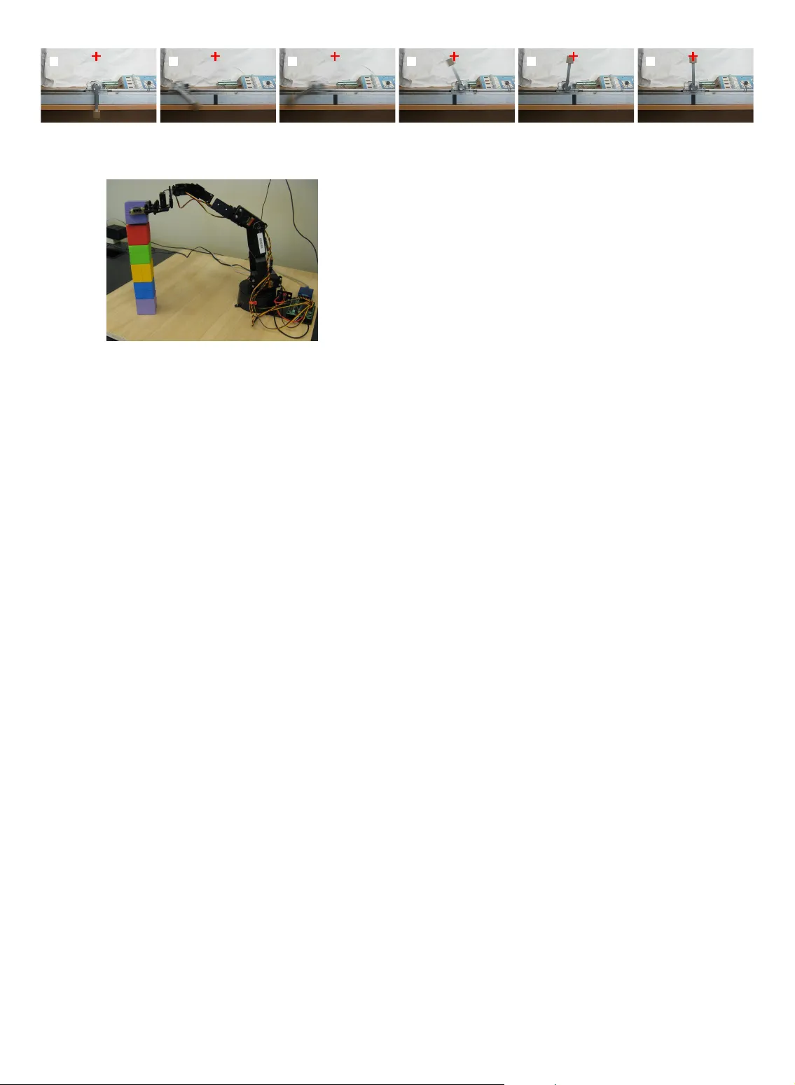
IEEE TRANSACTIONS ON P A TTERN ANAL YSIS AND MACHINE INTELLIGENCE, V OL. 37, NO. 2, FEBRU AR Y 2015 1 Gaussian Processes f or Data-Efﬁcient Lear ning in Robotics and Control Marc P eter Deisenroth, Dieter Fo x, and Carl Edward Rasm ussen Abstract —Autonomous learning has been a promising direction in control and robotics f or more than a decade since data-driven learning allows to reduce the amount of engineering knowledge, which is otherwise required. Howe v er , autonomous reinforcement learning (RL) approaches typically require many interactions with the system to learn controllers, which is a practical limitation in real systems, such as robots, where man y interactions can be impractical and time consuming. T o address this prob lem, current learning approaches typically require task-speciﬁc knowledge in f orm of expert demonstrations, realistic simulators, pre-shaped policies , or speciﬁc knowledge about the underlying dynamics. In this article, we follo w a diff erent approach and speed up learning by extr acting more information from data. In par ticular , we learn a probabilistic, non-parametric Gaussian process transition model of the system. By explicitly incorporating model uncertainty into long-ter m planning and controller lear ning our approach reduces the effects of model errors, a k ey prob lem in model-based learning. Compared to state-of-the ar t RL our model-based policy search method achieves an unprecedented speed of learning. We demonstrate its applicability to autonomous learning in real robot and control tasks. Index T erms —P olicy search, robotics, control, Gaussian processes, Ba yesian inf erence , reinforcement learning F 1 I N T R O D U C T I O N O N E of the main limitations of many current r ein- forcement learning (RL) algorithms is that learning is prohibitively slow , i.e., the requir ed number of interactions with the environment is impractically high. For example, many RL approaches in pr oblems with low-dimensional state spaces and fairly benign dynamics require thousands of trials to learn. This data inefﬁciency makes learning in real contr ol/r obotic systems impractical and prohibits RL approaches in more challenging scenarios. Increasing the data efﬁciency in RL requires either task- speciﬁc prior knowledge or extraction of more information from available data. In this article, we assume that expert knowledge (e.g., in terms of expert demonstrations [48], realistic simulators, or explicit differ ential equations for the dynamics) is unavaiable. Instead, we carefully model the observed dynamics using a general ﬂexible nonparametric approach. Generally , model-based methods, i.e., methods which learn an explicit dynamics model of the environment, are more promising to efﬁciently extract valuable information from available data [5] than model-free methods, such as • M.P . Deisenr oth is with the Department of Computing, Imperial College London, 180 Queen’ s Gate, London SW7 2AZ, United Kingdom, and with the Department of Computer Science, TU Darmstadt, Germany. • D. Fox is with the Department of Computer Science & Engineering, University of Washington, Box 352350, Seattle, W A 98195-2350. • C.E. Rasmussen is with the Department of Engineering, University of Cambridge, T rumpington Street, Cambridge CB2 1PZ, United Kingdom. Manuscript received 15 Sept. 2012; revised 6 May 2013; accepted 20 Oct. 2013; published online 4 November 2013. Recommended for acceptance by R.P . Adams, E. Fox, E. Sudderth, and Y .W . T eh. For information on obtaining reprints of this article, please send e-mail to: tpami@computer .org and refer ence IEEECS Log Number TP AMISI-2012-09-0742. Digital Object Identiﬁer no. 10.1109/TP AMI.2013.218 Q-learning [55] or TD-learning [52]. The main reason why model-based methods ar e not widely used in RL is that they can suffer severely from model errors , i.e., they inherently assume that the learned model resembles the real envi- ronment sufﬁciently accurately [5], [48], [49]. Model errors are especially an issue when only a few samples and no informative prior knowledge about the task are available. Fig. 1 illustrates how model err ors can af fect learning. Given a small data set of observed transitions (left), multiple transition functions plausibly could have generated them (center). Choosing a single deterministic model has severe consequences: Long-term predictions often leave the range of the training data in which case the pr edictions become es- sentially arbitrary . However , the deterministic model claims them with full conﬁdence! By contrast, a probabilistic model places a posterior distribution on plausible transition func- tions (right) and expresses the level of uncertainty about the model itself. When learning models, considerable model uncertainty is present, especially early on in learning. Thus, we require probabilistic models to express this uncertainty . Mor eover , model uncertainty needs to be incorporated into plan- ning and policy evaluation. Based on these ideas, we pro- pose P I L C O (Probabilistic Inference for Learning Control), a model-based policy search method [15], [16]. As a prob- abilistic model we use nonparametric Gaussian processes (GPs) [47]. P I L C O uses computationally efﬁcient determin- istic approximate inference for long-term predictions and policy evaluation. Policy improvement is based on ana- lytic policy gradients. Due to pr obabilistic modeling and inference P I L C O achieves unpr ecedented learning efﬁciency in continuous state-action domains and, hence, is directly applicable to complex mechanical systems, such as robots. In this article, we provide a detailed overview of the key ingredients of the P I L C O learning framework. In particular , we assess the quality of two dif ferent appr oximate infer ence IEEE TRANSACTIONS ON P A TTERN ANAL YSIS AND MACHINE INTELLIGENCE, V OL. 37, NO. 2, FEBRU AR Y 2015 2 −5 −4 −3 −2 −1 0 1 2 3 4 5 6 7 8 9 10 −2 0 2 (x t , u t ) f(x t , u t ) −5 −4 −3 −2 −1 0 1 2 3 4 5 6 7 8 9 10 −2 0 2 (x t , u t ) f(x t , u t ) −5 −4 −3 −2 −1 0 1 2 3 4 5 6 7 8 9 10 −2 0 2 (x t , u t ) f(x t , u t ) Fig. 1. Effect of model errors. Left: Small data set of obser ved transitions from an idealized one-dimensional representations of states and actions ( x t , u t ) to the ne xt state x t +1 = f ( x t , u t ) . Center: Multiple plausible deterministic models. Right: Probabilistic model. The probabilistic model describes the uncer tainty about the latent function by a probability distribution on the set of all plausible transition functions. Predictions with deterministic models are claimed with full conﬁdence, while the probabilistic model e xpresses its predictiv e uncertainty by a probability distribution. methods in the context of policy search. Moreover , we give a concrete example of the importance of Bayesian modeling and inference for fast learning from scratch. W e demon- strate that P I L C O ’s unpr ecedented learning speed makes it directly applicable to realistic control and robotic hardwar e platforms. This article is organized as follows: After discussing related work in Sec. 2, we describe the key ideas of the PI L C O learning framework in Sec. 3, i.e., the dynamics model, policy evaluation, and gradient-based policy improvement. In Sec. 4, we detail two approaches for long-term pr edictions for policy evaluation. In Sec. 5, we describe how the policy is repr esented and practically implemented. A particular cost function and its natural exploration/exploitation trade-off are discussed in Sec. 6. Experimental results are provided in Sec. 7. In Sec. 8, we discuss key properties, limitations, and extensions of the P I L C O framework before concluding in Sec. 9. 2 R E L AT E D W O R K Controlling systems under parameter uncertainty has been investigated for decades in robust and adaptive control [4], [35]. T ypically , a certainty equivalence principle is applied, which treats estimates of the model parameters as if they were the true values [58]. Approaches to designing adaptive controllers that explicitly take uncertainty about the model parameters into account are stochastic adaptive control [4] and dual control [23]. Dual contr ol aims to reduce parameter uncertainty by explicit probing, which is closely related to the exploration problem in RL. Robust, adaptive, and dual control are most often applied to linear systems [58]; nonlinear extensions exist in special cases [22]. The speciﬁcation of parametric models for a particular control problem is often challenging and requires intricate knowledge about the system. Sometimes, a r ough model estimate with uncertain parameters is sufﬁcient to solve challenging control problems. For instance, in [3], this ap- proach was applied together with locally optimal controllers and temporal bias terms for handling model errors. The key idea was to ground policy evaluations using real-life trials, but not the approximate model. All above-mentioned approaches to ﬁnding controllers requir e more or less accurate parametric models. These mod- els are problem speciﬁc and have to be manually speciﬁed, i.e., they ar e not suited for learning models for a br oad range of tasks. Nonparametric regression methods, however , are promising to automatically extract the important features of the latent dynamics from data. In [7], [49] locally weighted Bayesian regr ession was used as a nonparametric method for learning these models. T o deal with model uncertainty , in [7] model parameters were sampled from the parameter posterior , which accounts for temporal correlation. In [49], model uncertainty was treated as noise. The approach to controller learning was based on stochastic dynamic pro- gramming in discretized spaces, where the model errors at each time step were assumed independent. P I L C O builds upon the idea of treating model uncer- tainty as noise [49]. However , unlike [49], P I L C O is a policy search method and does not require state space discr etiza- tion. Instead closed-form Bayesian averaging over inﬁnitely many plausible dynamics models is possible by using non- parametric GPs. Nonparametric GP dynamics models in RL were previ- ously pr oposed in [17], [30], [46], where the GP training data were obtained from “motor babbling”. Unlike P I L C O , these approaches model global value functions to derive policies, requiring accurate value function models. T o reduce the effect of model err ors in the value functions, many data points are necessary as value functions ar e often discon- tinuous, rendering value-function based methods in high- dimensional state spaces often statistically and computa- tionally impractical. Therefor e, [17], [19], [46], [57] propose to learn GP value function models to address the issue of model errors in the value function. However , these methods can usually only be applied to low-dimensional RL prob- lems. As a policy search method, P I L C O does not require an explicit global value function model but rather searches directly in policy space. However , unlike value-function based methods, P I L C O is currently limited to episodic set- ups. 3 M O D E L - B A S E D P O L I C Y S E A R C H In this article, we consider dynamical systems x t +1 = f ( x t , u t ) + w , w ∼ N ( 0 , Σ w ) , (1) with continuous-valued states x ∈ R D and controls u ∈ R F , i.i.d. Gaussian system noise w , and unknown transition dynamics f . The policy search objective is to ﬁnd a policy/ controller π : x 7→ π ( x , θ ) = u , which minimizes the expected long-term cost J π ( θ ) = X T t =0 E x t [ c ( x t )] , x 0 ∼ N ( µ 0 , Σ 0 ) , (2) IEEE TRANSACTIONS ON P A TTERN ANAL YSIS AND MACHINE INTELLIGENCE, V OL. 37, NO. 2, FEBRU AR Y 2015 3 Algorithm 1 P I L C O 1: init: Sample controller parameters θ ∼ N ( 0 , I ) . Apply random control signals and record data. 2: repeat 3: Learn probabilistic (GP) dynamics model, see Sec. 3.1, using all data 4: repeat 5: Approximate inference for policy evaluation, see Sec. 3.2: get J π ( θ ) , Eq. (9)–(11) 6: Gradient-based policy improvement, see Sec. 3.3: get d J π ( θ ) / d θ , Eq. (12)–(16) 7: Update parameters θ (e.g., CG or L-BFGS). 8: until convergence; return θ ∗ 9: Set π ∗ ← π ( θ ∗ ) 10: Apply π ∗ to system and recor d data 11: until task learned of following π for T steps, where c ( x t ) is the cost of being in state x at time t . W e assume that π is a function parametrized by θ . 1 T o ﬁnd a policy π ∗ , which minimizes (2), P I L C O builds upon three components: 1) a probabilistic GP dynamics model (Sec. 3.1), 2) deterministic approximate inference for long-term pr edictions and policy evaluation (Sec. 3.2), 3) analytic computation of the policy gradients d J π ( θ ) / d θ for policy improvement (Sec. 3.3). The GP model inter- nally represents the dynamics in (1) and is subsequently employed for long-term predictions p ( x 1 | π ) , . . . , p ( x T | π ) , given a policy π . These predictions are obtained through approximate inference and used to evaluate the expected long-term cost J π ( θ ) in (2). The policy π is improved based on gradient information d J π ( θ ) / d θ . Alg. 1 summarizes the P I L C O learning framework. 3.1 Model Learning P I L C O ’s probabilistic dynamics model is implemented as a GP , where we use tuples ( x t , u t ) ∈ R D + F as training inputs and differences ∆ t = x t +1 − x t ∈ R D as training targets. 2 A GP is completely speciﬁed by a mean function m ( · ) and a positive semideﬁnite covariance function/kernel k ( · , · ) . In this paper , we consider a prior mean function m ≡ 0 and the covariance function k ( ˜ x p , ˜ x q ) = σ 2 f exp  − 1 2 ( ˜ x p − ˜ x q ) > Λ − 1 ( ˜ x p − ˜ x q )  + δ pq σ 2 w (3) with ˜ x : = [ x > u > ] > . W e deﬁned Λ : = diag([ ` 2 1 , . . . , ` 2 D + F ]) in (3), which depends on the characteristic length-scales ` i , and σ 2 f is the variance of the latent transition function f . Given n training inputs ˜ X = [ ˜ x 1 , . . . , ˜ x n ] and corre- sponding training targets y = [∆ 1 , . . . , ∆ n ] > , the posterior GP hyper-parameters (length-scales ` i , signal variance σ 2 f , and noise variance σ 2 w ) are learned by evidence maximiza- tion [34], [47]. 1. In our experiments in Sec. 7, we use a) nonlinear parametrizations by means of RBF networks, where the parameters θ are the weights and the features, or b) linear-afﬁne parametrizations, where the parameters θ are the weight matrix and a bias term. 2. Using dif ferences as training tar gets encodes an implicit prior mean function m ( x ) = x . This means that when leaving the training data, the GP predictions do not fall back to 0 but they remain constant. The posterior GP is a one-step prediction model, and the predicted successor state x t +1 is Gaussian distributed p ( x t +1 | x t , u t ) = N  x t +1 | µ t +1 , Σ t +1  (4) µ t +1 = x t + E f [ ∆ t ] , Σ t +1 = v ar f [ ∆ t ] , (5) where the mean and variance of the GP prediction are E f [ ∆ t ] = m f ( ˜ x t ) = k > ∗ ( K + σ 2 w I ) − 1 y = k > ∗ β , (6) v ar f [ ∆ t ] = k ∗∗ − k > ∗ ( K + σ 2 w I ) − 1 k ∗ , (7) respectively , with k ∗ : = k ( ˜ X , ˜ x t ) , k ∗∗ : = k ( ˜ x t , ˜ x t ) , and β : = ( K + σ 2 w I ) − 1 y , where K is the kernel matrix with entries K ij = k ( ˜ x i , ˜ x j ) . For multivariate targets, we train conditionally inde- pendent GPs for each target dimension, i.e., the GPs are independent for given test inputs. For uncertain inputs, the target dimensions covary [44], see also Sec. 4. 3.2 P olic y Evaluation T o evaluate and minimize J π in (2) P I L C O uses long- term predictions of the state evolution. In particular , we determine the marginal t -step-ahead predictive distribu- tions p ( x 1 | π ) , . . . , p ( x T | π ) fr om the initial state distribution p ( x 0 ) , t = 1 , . . . , T . T o obtain these long-term predictions, we cascade one-step predictions, see (4)–(5), which requires mapping uncertain test inputs through the GP dynamics model. In the following, we assume that these test inputs are Gaussian distributed. For notational convenience, we omit the explicit conditioning on the policy π in the fol- lowing and assume that episodes start from x 0 ∼ p ( x 0 ) = N  x 0 | µ 0 , Σ 0  . For predicting x t +1 from p ( x t ) , we requir e a joint distri- bution p ( ˜ x t ) = p ( x t , u t ) , see (1). The control u t = π ( x t , θ ) is a function of the state, and we approximate the desired joint distribution p ( ˜ x t ) = p ( x t , u t ) by a Gaussian. Details are provided in Sec. 5.5. From now on, we assume a joint Gaussian distribution distribution p ( ˜ x t ) = N  ˜ x t | ˜ µ t , ˜ Σ t  at time t . T o compute p ( ∆ t ) = Z Z p ( f ( ˜ x t ) | ˜ x t ) p ( ˜ x t ) d f d ˜ x t , (8) we integrate out both the random variable ˜ x t and the ran- dom function f , the latter one according to the posterior GP distribution. Computing the exact predictive distribution in (8) is analytically intractable as illustrated in Fig. 2. Hence, we approximate p ( ∆ t ) by a Gaussian. Assume the mean µ ∆ and the covariance Σ ∆ of the predictive distribution p ( ∆ t ) ar e known 3 . Then, a Gaussian approximation to the desired predictive distribution p ( x t +1 ) is given as N  x t +1 | µ t +1 , Σ t +1  with µ t +1 = µ t + µ ∆ , (9) Σ t +1 = Σ t + Σ ∆ + cov[ x t , ∆ t ] + cov[ ∆ t , x t ] . (10) Note that both µ ∆ and Σ ∆ are functions of the mean µ u and the covariance Σ u of the control signal. T o evaluate the expected long-term cost J π in (2), it remains to compute the expected values E x t [ c ( x t )] = Z c ( x t ) N  x t | µ t , Σ t  d x t , (11) 3. W e will detail their computations in Secs. 4.1–4.2. IEEE TRANSACTIONS ON P A TTERN ANAL YSIS AND MACHINE INTELLIGENCE, V OL. 37, NO. 2, FEBRU AR Y 2015 4 ∆ t ( x t , u t ) p ( x t , u t ) p ( ∆ t ) Ground truth Moment matching Linearization Fig. 2. GP prediction at an uncer tain input. The input distribution p ( x t , u t ) is assumed Gaussian (lower left panel). When propagating it through the GP model (upper left panel), we obtain the shaded distribu- tion p ( ∆ t ) , upper r ight panel. W e approximate p ( ∆ t ) by a Gaussian (upper r ight panel), which is computed by means of either moment matching (blue) or linearization of the poster ior GP mean (red). Using linearization for appro ximate inference can lead to predictive distr ibu- tions that are too tight. t = 1 , . . . , T , of the cost c with respect to the pr edictive state distributions. W e choose the cost c such that the integral in (11) and, thus, J π in (2) can computed analytically . Examples of such cost functions include polynomials and mixtures of Gaussians. 3.3 Analytic Gradients for Polic y Improvement T o ﬁnd policy parameters θ , which minimize J π ( θ ) in (2), we use gradient information d J π ( θ ) / d θ . W e require that the expected cost in (11) is differentiable with respect to the moments of the state distribution. Moreover , we assume that the moments of the control distribution µ u and Σ u can be computed analytically and are differentiable with respect to the policy parameters θ . In the following, we describe how to analytically com- pute these gradients for a gradient-based policy search. W e obtain the gradient d J π / d θ by repeated application of the chain-rule: First, we move the gradient into the sum in (2), and with E t : = E x t [ c ( x t )] we obtain d J π ( θ ) d θ = X T t =1 d E t d θ , d E t d θ = d E t d p ( x t ) d p ( x t ) d θ : = ∂ E t ∂ µ t d µ t d θ + ∂ E t ∂ Σ t d Σ t d θ , (12) where we used the shorthand notation d E t / d p ( x t ) = { d E t / d µ t , d E t / d Σ t } for taking the derivative of E t with respect to both the mean and covariance of p ( x t ) = N  x t | µ t , Σ t  . Second, as we will show in Sec. 4, the pre- dicted mean µ t and covariance Σ t depend on the moments of p ( x t − 1 ) and the controller parameters θ . By applying the chain-rule to (12), we obtain then d p ( x t ) d θ = ∂ p ( x t ) ∂ p ( x t − 1 ) d p ( x t − 1 ) d θ + ∂ p ( x t ) ∂ θ , (13) ∂ p ( x t ) ∂ p ( x t − 1 ) =  ∂ µ t ∂ p ( x t − 1 ) , ∂ Σ t ∂ p ( x t − 1 )  . (14) From here onward, we focus on d µ t / d θ , see (12), but com- puting d Σ t / d θ in (12) is similar . For d µ t / d θ , we compute the derivative d µ t d θ = ∂ µ t ∂ µ t − 1 d µ t − 1 d θ + ∂ µ t ∂ Σ t − 1 d Σ t − 1 d θ + ∂ µ t ∂ θ . (15) Since d p ( x t − 1 ) / d θ in (13) is known from time step t − 1 and ∂ µ t /∂ p ( x t − 1 ) is computed by applying the chain-rule to (17)–(20), we conclude with ∂ µ t ∂ θ = ∂ µ ∆ ∂ p ( u t − 1 ) ∂ p ( u t − 1 ) ∂ θ = ∂ µ ∆ ∂ µ u ∂ µ u ∂ θ + ∂ µ ∆ ∂ Σ u ∂ Σ u ∂ θ . (16) The partial derivatives of µ u and Σ u , i.e., the mean and covariance of p ( u t ) , used in (16) depend on the policy repr esentation. The individual partial derivatives in (12)– (16) depend on the approximate inference method used for propagating state distributions through time. For example, with moment matching or linearization of the posterior GP (see Sec. 4 for details) the desired gradients can be computed analytically by repeated application of the chain-rule. The Appendix derives the gradients for the moment-matching approximation. A gradient-based optimization method using estimates of the gradient of J π ( θ ) such as ﬁnite differences or more efﬁcient sampling-based methods (see [43] for an overview) requir es many function evaluations, which can be computa- tionally expensive. However , since in our case policy evalu- ation can be performed analytically , we proﬁt from analytic expressions for the gradients, which allows for standard gradient-based non-convex optimization methods, such as CG or BFGS, to determine optimized policy parameters θ ∗ . 4 L O N G - T E R M P R E D I C T I O N S Long-term predictions p ( x 1 ) , . . . , p ( x T ) for a given policy parametrization are essential for policy evaluation and im- provement as described in Secs. 3.2 and 3.3, respectively . These long-term predictions ar e computed iteratively: At each time step, P I L C O approximates the predictive state distribution p ( x t +1 ) by a Gaussian, see (9)–(10). For this approximation, we need to predict with GPs when the input is given by a probability distribution p ( ˜ x t ) , see (8). In this section, we detail the computations of the mean µ ∆ and covariance matrix Σ ∆ of the GP predic- tive distribution, see (8), as well as the cross-covariances co v[ ˜ x t , ∆ t ] = cov  [ x > t , u > t ] > , ∆ t  , which are requir ed in (9)–(10). W e present two approximations to predicting with GPs at uncertain inputs: Moment matching [15], [44] and linearization of the posterior GP mean function [28]. While moment matching computes the ﬁrst two moments of the predictive distribution exactly , their approximation by ex- plicit linearization of the posterior GP is computationally advantageous. 4.1 Moment Matching Following the law of iterated expectations, for tar get dimen- sions a = 1 , . . . , D , we obtain the predictive mean µ a ∆ = E ˜ x t [ E f a [ f a ( ˜ x t ) | ˜ x t ]] = E ˜ x t [ m f a ( ˜ x t )] = Z m f a ( ˜ x t ) N  ˜ x t | ˜ µ t , ˜ Σ t  d ˜ x t = β > a q a , (17) β a = ( K a + σ 2 w a ) − 1 y a , (18) IEEE TRANSACTIONS ON P A TTERN ANAL YSIS AND MACHINE INTELLIGENCE, V OL. 37, NO. 2, FEBRU AR Y 2015 5 with q a = [ q a 1 , . . . , q a n ] > . The entries of q a ∈ R n are computed using standard results from multiplying and integrating over Gaussians and are given by q a i = Z k a ( ˜ x i , ˜ x t ) N  ˜ x t | ˜ µ t , ˜ Σ t  d ˜ x t (19) = σ 2 f a | ˜ Σ t Λ − 1 a + I | − 1 2 exp  − 1 2 ν > i ( ˜ Σ t + Λ a ) − 1 ν i  , where we deﬁne ν i : = ( ˜ x i − ˜ µ t ) (20) as the differ ence between the training input ˜ x i and the mean of the test input distribution p ( x t , u t ) . Computing the predictive covariance matrix Σ ∆ ∈ R D × D requir es us to distinguish between diagonal elements σ 2 aa and off-diagonal elements σ 2 ab , a 6 = b : Using the law of total (co-)variance, we obtain for target dimensions a, b = 1 , . . . , D σ 2 aa = E ˜ x t  v ar f [∆ a | ˜ x t ]  + E f , ˜ x t [∆ 2 a ] − ( µ a ∆ ) 2 , (21) σ 2 ab = E f , ˜ x t [∆ a ∆ b ] − µ a ∆ µ b ∆ , a 6 = b , (22) respectively , where µ a ∆ is known from (17). The off- diagonal terms σ 2 ab do not contain the additional term E ˜ x t [co v f [∆ a , ∆ b | ˜ x t ]] because of the conditional indepen- dence assumption of the GP models: Dif ferent target dimen- sions do not covary for given ˜ x t . W e start the computation of the covariance matrix with the terms that are common to both the diagonal and the off- diagonal entries: W ith p ( ˜ x t ) = N  ˜ x t | ˜ µ t , ˜ Σ t  and the law of iterated expectations, we obtain E f , ˜ x t [∆ a ∆ b ] = E ˜ x t  E f [∆ a | ˜ x t ] E f [∆ b | ˜ x t ]  (6) = Z m a f ( ˜ x t ) m b f ( ˜ x t ) p ( ˜ x t ) d ˜ x t (23) because of the conditional independence of ∆ a and ∆ b given ˜ x t . Using the deﬁnition of the GP mean function in (6), we obtain E f , ˜ x t [∆ a ∆ b ] = β > a Qβ b , (24) Q : = Z k a ( ˜ x t , ˜ X ) > k b ( ˜ x t , ˜ X ) p ( ˜ x t ) d ˜ x t . (25) Using standard results from Gaussian multiplications and integration, we obtain the entries Q ij of Q ∈ R n × n Q ij = | R | − 1 2 k a ( ˜ x i , ˜ µ t ) k b ( ˜ x j , ˜ µ t ) exp  1 2 z > ij T − 1 z ij  (26) where we deﬁne R : = ˜ Σ t ( Λ − 1 a + Λ − 1 b ) + I , T : = Λ − 1 a + Λ − 1 b + ˜ Σ − 1 t , z ij : = Λ − 1 a ν i + Λ − 1 b ν j , with ν i deﬁned in (20). Hence, the off-diagonal entries of Σ ∆ are fully determined by (17)–(20), (22), and (24)–(26). From (21), we see that the diagonal entries contain the additional term E ˜ x t  v ar f [∆ a | ˜ x t ]  = σ 2 f a − tr  ( K a + σ 2 w a I ) − 1 Q  + σ 2 w a (27) with Q given in (26) and σ 2 w a being the system noise vari- ance of the a th target dimension. This term is the expected variance of the function, see (7), under the distribution p ( ˜ x t ) . T o obtain the cross-covariances cov[ x t , ∆ t ] in (10), we compute the cross-covariance co v[ ˜ x t , ∆ t ] between an uncer- tain state-action pair ˜ x t ∼ N ( ˜ µ t , ˜ Σ t ) and the corr esponding predicted state differ ence x t +1 − x t = ∆ t ∼ N ( µ ∆ , Σ ∆ ) . This cross-covariance is given by co v[ ˜ x t , ∆ t ] = E ˜ x t ,f [ ˜ x t ∆ > t ] − ˜ µ t µ > ∆ , (28) where the components of µ ∆ are given in (17), and ˜ µ t is the known mean of the input distribution of the state-action pair at time step t . Using the law of iterated expectation, for each state dimension a = 1 , . . . , D , we compute E ˜ x t ,f [ ˜ x t ∆ a t ] as E ˜ x t ,f [ ˜ x t ∆ a t ] = E ˜ x t [ ˜ x t E f [∆ a t | ˜ x t ]] = Z ˜ x t m a f ( ˜ x t ) p ( ˜ x t ) d ˜ x t (6) = Z ˜ x t  n X i =1 β a i k a f ( ˜ x t , ˜ x i )  p ( ˜ x t ) d ˜ x t , (29) where the (posterior) GP mean function m f ( ˜ x t ) was rep- resented as a ﬁnite kernel expansion. Note that ˜ x i are the state-action pairs, which were used to train the dynamics GP model. By pulling the constant β a i out of the integral and changing the order of summation and integration, we obtain E ˜ x t ,f [ ˜ x t ∆ a t ] = n X i =1 β a i Z ˜ x t c 1 N ( ˜ x t | ˜ x i , Λ a ) | {z } = k a f ( ˜ x t , ˜ x i ) N ( ˜ x t | ˜ µ t , ˜ Σ t ) | {z } p ( ˜ x t ) d ˜ x t , (30) where we deﬁne c 1 : = σ 2 f a (2 π ) D + F 2 | Λ a | 1 2 with ˜ x ∈ R D + F , such that k a f ( ˜ x t , ˜ x i ) = c 1 N  ˜ x t | ˜ x i , Λ a  is an unnormal- ized Gaussian probability distribution in ˜ x t , where ˜ x i , i = 1 , . . . , n , are the GP training inputs. The product of the two Gaussians in (30) yields a new (unnormalized) Gaussian c − 1 2 N  ˜ x t | ψ i , Ψ  with c − 1 2 = (2 π ) − D + F 2 | Λ a + ˜ Σ t | − 1 2 × exp  − 1 2 ( ˜ x i − ˜ µ t ) > ( Λ a + ˜ Σ t ) − 1 ( ˜ x i − ˜ µ t )  , Ψ = ( Λ − 1 a + ˜ Σ − 1 t ) − 1 , ψ i = Ψ ( Λ − 1 a ˜ x i + ˜ Σ − 1 t ˜ µ t ) . By pulling all remaining variables, which are independent of ˜ x t , out of the integral in (30), the integral determines the expected value of the product of the two Gaussians, ψ i . Hence, we obtain E ˜ x t ,f [ ˜ x t ∆ a t ] = X n i =1 c 1 c − 1 2 β a i ψ i , a = 1 , . . . , D , co v ˜ x t ,f [ ˜ x t , ∆ a t ] = X n i =1 c 1 c − 1 2 β a i ψ i − ˜ µ t µ a ∆ , (31) for all predictive dimensions a = 1 , . . . , E . W ith c 1 c − 1 2 = q a i , see (19), and ψ i = ˜ Σ t ( ˜ Σ t + Λ a ) − 1 ˜ x i + Λ ( ˜ Σ t + Λ a ) − 1 ˜ µ t we simplify (31) and obtain co v ˜ x t ,f [ ˜ x t , ∆ a t ] = n X i =1 β a i q a i ˜ Σ t ( ˜ Σ t + Λ a ) − 1 ( ˜ x i − ˜ µ t ) , (32) a = 1 , . . . , E . The desired covariance cov[ x t , ∆ t ] is a D × E submatrix of the ( D + F ) × E cross-covariance computed in to (32). A visualization of the approximation of the predictive distribution by means of exact moment matching is given in Fig. 2. IEEE TRANSACTIONS ON P A TTERN ANAL YSIS AND MACHINE INTELLIGENCE, V OL. 37, NO. 2, FEBRU AR Y 2015 6 4.2 Linearization of the Posterior GP Mean Function An alternative way of approximating the predictive distri- bution p ( ∆ t ) by a Gaussian for ˜ x t ∼ N  ˜ x t | ˜ µ t , ˜ Σ t  is to linearize the posterior GP mean function. Fig. 2 visualizes the approximation by means of linearizing the posterior GP mean function. The predicted mean is obtained by evaluating the posterior GP mean in (5) at the mean ˜ µ t of the input distribution, i.e., µ a ∆ = E f [ f a ( ˜ µ t )] = m f a ( ˜ µ t ) = β > a k a ( ˜ X , ˜ µ t ) , (33) a = 1 , . . . , E , where β a is given in (18). T o compute the GP predictive covariance matrix Σ ∆ , we explicitly linearize the posterior GP mean function around ˜ µ t . By applying standard results for mapping Gaussian dis- tributions through linear models, the predictive covariance is given by Σ ∆ = V ˜ Σ t V > + Σ w , (34) V = ∂ µ ∆ ∂ ˜ µ t = β > ∂ k ( ˜ X , ˜ µ t ) ∂ ˜ µ t . (35) In (34), Σ w is a diagonal matrix whose entries are the noise variances σ 2 w a plus the model uncertainties v ar f [∆ a t | ˜ µ t ] evaluated at ˜ µ t , see (7). This means, model uncertainty no longer depends on the density of the data points. Instead it is assumed to be constant. Note that the moments computed in (33)–(34) are not exact. The cross-covariance co v[ ˜ x t , ∆ t ] is given by ˜ Σ t V , where V is deﬁned in (35). 5 P O L I C Y In the following, we describe the desired properties of the policy within the P I L C O learning framework. First, to compute the long-term predictions p ( x 1 ) , . . . , p ( x T ) for policy evaluation, the policy must allow us to compute a distribution over contr ols p ( u ) = p ( π ( x )) for a given (Gaussian) state distribution p ( x ) . Second, in a r ealistic real- world application, the amplitudes of the control signals are bounded. Ideally , the learning system takes these constraints explicitly into account. In the following, we detail how P I L C O implements these desiderata. 5.1 Predictive Distribution over Controls During the long-term predictions, the states are given by a probability distribution p ( x t ) , t = 0 , . . . , T . The probability distribution of the state x t induces a predictive distribution p ( u t ) = p ( π ( x t )) over controls, even when the policy is deterministic. W e appr oximate the distribution over controls using moment matching, which is in many interesting cases analytically tractable. 5.2 Constrained Control Signals In practical applications, force or torque limits are present and must be accounted for during planning. Suppose the control limits are such that u ∈ [ − u max , u max ] . Let us consider a preliminary policy ˜ π with an unconstrained am- plitude. T o account for the control limits coherently during simulation, we squash the preliminary policy ˜ π through a bounded and differentiable squashing function, which −5 0 5 −1 0 1 2 x ˜ π ( x ) (a) Preliminar y policy ˜ π as a func- tion of the state. −5 0 5 −1 0 1 2 x π ( x ) (b) Policy π = σ ( ˜ π ( x )) as a func- tion of the state. Fig. 3. Constr aining the control signal. P anel (a) shows an e xample of an unconstrained preliminary policy ˜ π as a function of the state x . P anel (b) shows the constrained policy π ( x ) = σ ( ˜ π ( x )) as a function of the state x . limits the amplitude of the ﬁnal policy π . As a squashing function, we use σ ( x ) = 9 8 sin( x ) + 1 8 sin(3 x ) ∈ [ − 1 , 1] , (36) which is the third-order Fourier series expansion of a trape- zoidal wave, normalized to the interval [ − 1 , 1] . The squash- ing function in (36) is computationally convenient as we can analytically compute predictive moments for Gaussian distributed states. Subsequently , we multiply the squashed policy by u max and obtain the ﬁnal policy π ( x ) = u max σ ( ˜ π ( x )) ∈ [ − u max , u max ] , (37) an illustration of which is shown in Fig. 3. Although the squashing function in (36) is periodic, it is almost always used within a half wave if the preliminary policy ˜ π is initialized to produce function values that do not exceed the domain of a single period. Therefor e, the periodicity does not matter in practice. T o compute a distribution over constrained control sig- nals, we execute the following steps: p ( x t ) 7→ p ( ˜ π ( x t )) 7→ p ( u max σ ( ˜ π ( x t ))) = p ( u t ) . (38) First, we map the Gaussian state distribution p ( x t ) thr ough the preliminary (unconstrained) policy ˜ π . Thus, we requir e a preliminary policy ˜ π that allows for closed-form com- putation of the moments of the distribution over controls p ( ˜ π ( x t )) . Second, we squash the approximate Gaussian distribution p ( ˜ π ( x )) according to (37) and compute exactly the mean and variance of p ( ˜ π ( x )) . Details are given in the Appendix. W e approximate p ( ˜ π ( x )) by a Gaussian with these moments, yielding the distribution p ( u ) over controls in (38). 5.3 Representations of the Preliminar y P olicy In the following, we present two repr esentations of the preliminary policy ˜ π , which allow for closed-form computa- tions of the mean and covariance of p ( ˜ π ( x )) when the state x is Gaussian distributed. W e consider both a linear and a nonlinear representations of ˜ π . 5.3.1 Linear P olicy The linear preliminary policy is given by ˜ π ( x ∗ ) = Ax ∗ + b , (39) where A is a parameter matrix of weights and b is an offset vector . In each control dimension d , the policy in (39) is a IEEE TRANSACTIONS ON P A TTERN ANAL YSIS AND MACHINE INTELLIGENCE, V OL. 37, NO. 2, FEBRU AR Y 2015 7 linear combination of the states (the weights are given by the d th row in A ) plus an offset b d . The predictive distribution p ( ˜ π ( x ∗ )) for a state distribu- tion x ∗ ∼ N ( µ ∗ , Σ ∗ ) is an exact Gaussian with mean and covariance E x ∗ [ ˜ π ( x ∗ )] = Aµ ∗ + b , cov x ∗ [ ˜ π ( x ∗ )] = A Σ ∗ A > , (40) respectively . A drawback of the linear policy is that it is not ﬂexible. However , a linear controller can often be used for stabilization around an equilibrium. 5.3.2 Nonlinear P olicy: Deter ministic Gaussian Process In the nonlinear case, we represent the preliminary policy ˜ π by ˜ π ( x ∗ ) = N X i =1 k ( m i , x ∗ )( K + σ 2 π I ) − 1 t = k ( M , x ∗ ) > α , (41) where x ∗ is a test input, α = ( K + 0 . 01 I ) − 1 t , where t plays the role of a GP’s training targets. In (41), M = [ m 1 , . . . , m N ] ar e the centers of the (axis-aligned) Gaussian basis functions k ( x p , x q ) = exp  − 1 2 ( x p − x q ) > Λ − 1 ( x p − x q )  . (42) W e call the policy representation in (41) a deterministic GP with a ﬁxed number of N basis functions. Here, “determin- istic” means that there is no uncertainty about the under- lying function, that is, v ar ˜ π [ ˜ π ( x )] = 0 . Therefore, the de- terministic GP is a degenerate model, which is functionally equivalent to a regularized RBF network. The deterministic GP is functionally equivalent to the posterior GP mean function in (6), where we set the signal variance to 1, see (42), and the noise variance to 0 . 01 . As the pr eliminary policy will be squashed through σ in (36) whose relevant support is the interval [ − π 2 , π 2 ] , a signal variance of 1 is about right. Setting additionally the noise standard deviation to 0.1 corr esponds to ﬁxing the signal-to-noise ratio of the policy to 10 and, hence, the regularization. For a Gaussian distributed state x ∗ ∼ N ( µ ∗ , Σ ∗ ) , the predictive mean of ˜ π ( x ∗ ) as deﬁned in (41) is given as E x ∗ [ ˜ π ( x ∗ )] = α > a E x ∗ [ k ( M , x ∗ )] = α > a Z k ( M , x ∗ ) p ( x ∗ ) d x ∗ = α > a r a , (43) where for i = 1 , . . . , N and all policy dimensions a = 1 , . . . , F r a i = | Σ ∗ Λ − 1 a + I | − 1 2 × exp( − 1 2 ( µ ∗ − m i ) > ( Σ ∗ + Λ a ) − 1 ( µ ∗ − m i )) . The diagonal matrix Λ a contains the squared length-scales ` i , i = 1 , . . . , D . The predicted mean in (43) is equivalent to the standard predicted GP mean in (17). For a, b = 1 , . . . , F , the entries of the predictive covariance matrix are computed according to co v x ∗ [ ˜ π a ( x ∗ ) , ˜ π b ( x ∗ )] = E x ∗ [ ˜ π a ( x ∗ ) ˜ π b ( x ∗ )] − E x ∗ [ ˜ π a ( x ∗ )] E x ∗ [ ˜ π b ( x ∗ )] , Algorithm 2 Computing the Successor State Distribution 1: init: x t ∼ N ( µ t , Σ t ) 2: Control distribution p ( u t ) = p ( u max σ ( ˜ π ( x t , θ ))) 3: Joint state-control distribution p ( ˜ x t ) = p ( x t , u t ) 4: Predictive GP distribution of change in state p ( ∆ t ) 5: Distribution of successor state p ( x t +1 ) where E x ∗ [ ˜ π { a,b } ( x ∗ )] is given in (43). Hence, we focus on the term E x ∗ [ ˜ π a ( x ∗ ) ˜ π b ( x ∗ )] , which for a, b = 1 , . . . , F is given by E x ∗ [ ˜ π a ( x ∗ ) ˜ π b ( x ∗ )] = α > a E x ∗ [ k a ( M , x ∗ ) k b ( M , x ∗ ) > ] α b = α > a Qα b . For i, j = 1 , . . . , N , we compute the entries of Q as Q ij = Z k a ( m i , x ∗ ) k b ( m j , x ∗ ) p ( x ∗ ) d x ∗ = k a ( m i , µ ∗ ) k b ( m j , µ ∗ ) | R | − 1 2 exp( 1 2 z > ij T − 1 z ij ) , R = Σ ∗ ( Λ − 1 a + Λ − 1 b ) + I , T = Λ − 1 a + Λ − 1 b + Σ − 1 ∗ , z ij = Λ − 1 a ( µ ∗ − m i ) + Λ − 1 b ( µ ∗ − m j ) . Combining this result with (43) fully determines the predic- tive covariance matrix of the preliminary policy . Unlike the predictive covariance of a probabilistic GP , see (21)–(22), the predictive covariance matrix of the deter- ministic GP does not comprise any model uncertainty in its diagonal entries. 5.4 P olic y Parameters In the following, we describe the policy parameters for both the linear and the nonlinear policy 4 . 5.4.1 Linear P olicy The linear policy in (39) possesses D + 1 parameters per control dimension: For control dimension d there are D weights in the d th row of the matrix A . One additional parameter originates from the offset parameter b d . 5.4.2 Nonlinear P olicy The parameters of the deterministic GP in (41) are the locations M of the centers ( D N parameters), the (shared) length-scales of the Gaussian basis functions ( D length-scale parameters per target dimension), and the N tar gets t per target dimension. In the case of multivariate controls, the basis function centers M are shared. 5.5 Computing the Successor State Distribution Alg. 2 summarizes the computational steps requir ed to compute the successor state distribution p ( x t +1 ) from p ( x t ) . The computation of a distribution over controls p ( u t ) from the state distribution p ( x t ) requires two steps: First, for a Gaussian state distribution p ( x t ) at time t a Gaussian ap- proximation of the distribution p ( ˜ π ( x t )) of the preliminary policy is computed analytically . Second, the preliminary 4. For notational convenience, with a (non)linear policy we mean the (non)linear preliminary policy ˜ π mapped through the squashing function σ and subsequently multiplied by u max . IEEE TRANSACTIONS ON P A TTERN ANAL YSIS AND MACHINE INTELLIGENCE, V OL. 37, NO. 2, FEBRU AR Y 2015 8 policy is squashed through σ and an approximate Gaussian distribution of p ( u max σ ( ˜ π ( x t ))) is computed analytically in (38) using results from the Appendix. Third, we analytically compute a Gaussian approximation to the joint distribution p ( x t , u t ) = p ( x t , π ( x t )) . For this, we compute (a) a Gaus- sian approximation to the joint distribution p ( x t , ˜ π ( x t )) , which is exact if ˜ π is linear , and (b) an approximate fully joint Gaussian distribution p ( x t , ˜ π ( x t ) , u t ) . W e obtain cr oss- covariance information between the state x t and the control signal u t = u max σ ( ˜ π ( x t )) via co v[ x t , u t ] = cov[ x t , ˜ π ( x t )]co v[ ˜ π ( x t ) , ˜ π ( x t )] − 1 co v[ ˜ π ( x t ) , u t ] , where we exploit the conditional independence of x t and u t given ˜ π ( x t ) . Then, we integrate ˜ π ( x t ) out to obtain the desired joint distribution p ( x t , u t ) . This leads to an approx- imate Gaussian joint probability distribution p ( x t , u t ) = p ( x t , π ( x t )) = p ( ˜ x t ) . Fourth, with the approximate Gaus- sian input distribution p ( ˜ x t ) , the distribution p ( ∆ t ) of the change in state is computed using the results from Sec. 4. Finally , the mean and covariance of a Gaussian approxima- tion of the successor state distribution p ( x t +1 ) are given by (9) and (10), respectively . All r equired computations can be performed analytically because of the choice of the Gaussian covariance function for the GP dynamics model, see (3), the representations of the preliminary policy ˜ π , see Sec. 5.3, and the choice of the squashing function, see (36). 6 C O S T F U N C T I O N In our learning set-up, we use a cost function that solely penalizes the Euclidean distance d of the current state to the target state. Using only distance penalties is often sufﬁcient to solve a task: Reaching a target x target with high speed naturally leads to overshooting and, thus, to high long-term costs. In particular , we use the generalized binary saturating cost c ( x ) = 1 − exp  − 1 2 σ 2 c d ( x , x target ) 2  ∈ [0 , 1] , (44) which is locally quadratic but saturates at unity for large deviations d from the desired target x target . In (44), the geometric distance fr om the state x to the tar get state is denoted by d , and the parameter σ c controls the width of the cost function. 5 In classical contr ol, typically a quadratic cost is assumed. However , a quadratic cost tends to focus attention on the worst deviation from the target state along a predicted trajectory . In the early stages of learning the predictive un- certainty is large and, therefore, the policy gradients, which are described in Sec. 3.3 become less useful. Therefor e, we use the saturating cost in (44) as a default within the P I L C O learning framework. The immediate cost in (44) is an unnormalized Gaussian with mean x target and variance σ 2 c , subtracted from unity . 5. In the context of sensorimotor control, the saturating cost function in (44) resembles the cost function in human reasoning as experimen- tally validated by [31]. −1.5 −1 −0.5 0 0.5 1 1.5 0 0.5 1 1.5 2 2.5 state cost function peaked state distribution wide state distribution (a) When the mean of the state is far a wa y from the target, uncertain states (red, dashed-dotted) are preferred to more cer tain states with a more peaked distr ibution (blac k, dashed). This leads to ini- tial explor ation. −1.5 −1 −0.5 0 0.5 1 1.5 0 0.5 1 1.5 2 2.5 state cost function peaked state distribution wide state distribution (b) When the mean of the state is close to the target, peaked state distributions (black, dashed) cause less expected cost and, thus, are pref er able to more uncer- tain states (red, dashed-dotted), leading to exploitation close to the target. Fig. 4. A utomatic exploration and exploitation with the saturating cost function (blue, solid). The x -axes descr ibe the state space. The target state is the origin. Therefor e, the expected immediate cost can be computed analytically according to E x [ c ( x )] = Z c ( x ) p ( x ) d x (45) = 1 − Z exp  − 1 2 ( x − x target ) > T − 1 ( x − x target )  p ( x ) d x , where T − 1 is the precision matrix of the unnormalized Gaussian in (45). If the state x has the same repr esentation as the target vector , T − 1 is a diagonal matrix with entries either unity or zero, scaled by 1 /σ 2 c . Hence, for x ∼ N ( µ , Σ ) we obtain the expected immediate cost E x [ c ( x )] = 1 − | I + Σ T − 1 | − 1 / 2 × exp( − 1 2 ( µ − x target ) > ˜ S 1 ( µ − x target )) , (46) ˜ S 1 : = T − 1 ( I + Σ T − 1 ) − 1 . (47) The partial derivatives ∂ ∂ µ t E x t [ c ( x t )] , ∂ ∂ Σ t E x t [ c ( x t )] of the immediate cost with respect to the mean and the covariance of the state distribution p ( x t ) = N ( µ t , Σ t ) , which are requir ed to compute the policy gradients analytically , are given by ∂ E x t [ c ( x t )] ∂ µ t = − E x t [ c ( x t )] ( µ t − x target ) > ˜ S 1 , (48) ∂ E x t [ c ( x t )] ∂ Σ t = 1 2 E x t [ c ( x t )] (49) ×  ˜ S 1 ( µ t − x target )( µ t − x target ) > − I  ˜ S 1 , respectively , where ˜ S 1 is given in (47). 6.1 Exploration and Exploitation The saturating cost function in (44) allows for a natural exploration when the policy aims to minimize the expected long-term cost in (2). This property is illustrated in Fig. 4 for a single time step where we assume a Gaussian state distribution p ( x t ) . If the mean of p ( x t ) is far away from the target x target , a wide state distribution is more likely to have substantial tails in some low-cost region than a more peaked distribution as shown in Fig. 4(a). In the IEEE TRANSACTIONS ON P A TTERN ANAL YSIS AND MACHINE INTELLIGENCE, V OL. 37, NO. 2, FEBRU AR Y 2015 9 early stages of learning, the predictive state uncertainty is largely due to propagating model uncertainties forward. If we predict a state distribution in a high-cost region, the sat- urating cost then leads to automatic exploration by favoring uncertain states, i.e., states in regions far from the target with a poor dynamics model. When visiting these regions during interaction with the physical system, subsequent model learning reduces the model uncertainty locally . In the subsequent policy evaluation, P I L C O will predict a tighter state distribution in the situations described in Fig. 4. If the mean of the state distribution is close to the target as in Fig. 4(b), wide distributions are likely to have substantial tails in high-cost regions. By contrast, the mass of a peaked distribution is mor e concentrated in low-cost regions. In this case, the policy prefers peaked distributions close to the target, leading to exploitation . T o summarize, combining a probabilistic dynamics model, Bayesian inference, and a saturating cost leads to automatic exploration as long as the pr edictions ar e far fr om the target—even for a policy , which greedily minimizes the expected cost. Once close to the target, the policy does not substantially deviate from a conﬁdent trajectory that leads the system close to the target. 6 7 E X P E R I M E N TA L R E S U L T S In this section, we assess P I L C O ’s key properties and show that P I L C O scales to high-dimensional control problems. Moreover , we demonstrate the hardware applicability of our learning framework on two real systems. In all cases, P I L C O followed the steps outlined in Alg. 1. T o reduce the computational burden, we used the sparse GP method of [50] after 300 collected data points. 7.1 Ev aluation of Key Properties In the following, we assess the quality of the approximate inference method used for long-term predictions in terms of computational demand and learning speed. Moreover , we shed some light on the quality of the Gaussian approxima- tions of the predictive state distributions and the importance of Bayesian averaging. For these assessments, we applied P I L C O to two nonlinear control tasks, which are introduced in the following. 7.1.1 T ask Descriptions W e considered two simulated tasks (double-pendulum swing-up, cart-pole swing-up) to evaluate important prop- erties of the P I L C O policy search framework: learning speed, quality of approximate inference, importance of Bayesian averaging, and hardware applicability . In the following we brieﬂy introduce the experimental set-ups. 7.1.1.1 Double-Pendulum Swing-Up with T wo Ac- tuators: The double pendulum system is a two-link robot arm with two actuators, see Fig. 5. The state x is given by the angles θ 1 , θ 2 and the corresponding angular velocities ˙ θ 1 , ˙ θ 2 of the inner and outer link, respectively , measured fr om being upright. Each link was of length 1 m and mass 0 . 5 kg . Both torques u 1 and u 2 were constrained to [ − 3 , 3] Nm . The control signal could be changed every 100 ms . In the 6. Code is available at http://mloss.org/software/view/508/ . target u 1 u 2 d Fig. 5. Double pendulum with two actuators applying torques u 1 and u 2 . The cost function penalizes the distance d to the target. meantime it was constant (zero-or der-hold control). The objective was to learn a controller that swings the double pendulum up from an initial distribution p ( x 0 ) around µ 0 = [ π , π , 0 , 0] > and balances it in the inverted position with θ 1 = 0 = θ 2 . The prediction horizon was 2 . 5 s . The task is challenging since its solution requir es the in- terplay of two correlated control signals. The challenge is to automatically learn this interplay from experience. T o solve the double pendulum swing-up task, a nonlinear policy is requir ed. Thus, we parametrized the preliminary policy as a deterministic GP , see (41), with 100 basis functions resulting in 812 policy parameters. W e chose the saturating immediate cost in (44), where the Euclidean distance between the upright position and the tip of the outer link was penalized. W e chose the cost width σ c = 0 . 5 , which means that the tip of the outer pendulum had to cross horizontal to achieve an immediate cost smaller than unity . 7.1.1.2 Cart-Pole Swing-Up : The cart-pole system consists of a cart running on a track and a freely swing- ing pendulum attached to the cart. The state of the sys- tem is the position x of the cart, the velocity ˙ x of the cart, the angle θ of the pendulum measured from hanging downward, and the angular velocity ˙ θ . A horizontal force u ∈ [ − 10 , 10] N could be applied to the cart. The objective was to learn a controller to swing the pendulum up from around µ 0 = [ x 0 , ˙ x 0 , θ 0 , ˙ θ 0 ] > = [0 , 0 , 0 , 0] > and to balance it in the inverted position in the middle of the track, i.e., around x target = [0 , ∗ , π , ∗ ] > . Since a linear controller is not capable of solving the task [45], P I L C O learned a nonlinear state-feedback controller based on a deterministic GP with 50 basis functions (see Sec. 5.3.2), resulting in 305 policy parameters to be learned. In our simulation, we set the masses of the cart and the pendulum to 0 . 5 kg each, the length of the pendulum to 0 . 5 m , and the coefﬁcient of friction between cart and ground to 0 . 1 Ns / m . The prediction horizon was set to 2 . 5 s . The control signal could be changed every 100 ms . In the meantime, it was constant (zero-order -hold control). The only knowledge employed about the system was the length of the pendulum to ﬁnd appropriate orders of magnitude to set the sampling frequency ( 10 Hz ) and the standard deviation of the cost function ( σ c = 0 . 25 m ), requiring the tip of the pendulum to move above horizontal not to incur full cost. IEEE TRANSACTIONS ON P A TTERN ANAL YSIS AND MACHINE INTELLIGENCE, V OL. 37, NO. 2, FEBRU AR Y 2015 10 5 10 15 20 25 30 35 40 45 50 10 −2 10 0 10 2 State space dimensionality Computation time in s 100 Training Points 250 Training Points 500 Training Points 1000 Training Points (a) Linearizing the mean function. 5 10 15 20 25 30 35 40 45 50 10 −2 10 0 10 2 State space dimensionality Computation time in s 100 Training Points 250 Training Points 500 Training Points 1000 Training Points (b) Moment matching. Fig. 6. Empir ical computational demand for approximate inference and derivativ e computation with GPs for a single time step, shown on a log scale. (a): Linearization of the poster ior GP mean. (b): Exact moment matching. 7.1.2 Appro ximate Inference Assessment In the following, we evaluate the quality of the presented approximate inference methods for policy evaluation (mo- ment matching as described in Sec. 4.1) and linearization of the posterior GP mean as described in Sec. 4.2) with respect to computational demand (Sec. 7.1.2.1) and learning speed (Sec. 7.1.2.2). 7.1.2.1 Computational Demand: For a single time step, the computational complexity of moment matching is O ( n 2 E 2 D ) , where n is the number of GP training points, D is the input dimensionality , and E the dimension of the prediction. The most expensive computations are the entries of Q ∈ R n × n , which are given in (26). Each entry Q ij requir es evaluating a kernel, which is essentially a D - dimensional scalar product. The values z ij are cheap to compute and R needs to be computed only once. W e end up with O ( n 2 E 2 D ) since Q needs to be computed for all entries of the E × E predictive covariance matrix. For a single time step, the computational complexity of linearizing the posterior GP mean function is O ( n 2 D E ) . The most expensive operation is the determination of Σ w in (34), i.e., the model uncertainty at the mean of the input distribution, which scales in O ( n 2 D ) . This computation is performed for all E predictive dimensions, resulting in a computational complexity of O ( n 2 D E ) . Fig. 6 illustrates the empirical computational effort for both linearization of the posterior GP mean and exact moment matching. W e randomly generated GP models in D = 1 , 2 , 3 , 4 , 5 , 6 , 7 , 8 , 9 , 10 , 15 , 20 , 50 dimensions and GP training set sizes of n = 100 , 250 , 500 , 1000 data points. W e set the predictive dimension E = D . The CPU time (single core) for computing a predictive state distribution and the requir ed derivatives are shown as a function of the dimensionality of the state. Four graphs are shown for set-ups with 100, 250, 500, and 1000 GP training points, respectively . Fig. 6(a) shows the graphs for approximate inference based on linearization of the posterior GP mean, and Fig. 6(b) shows the corresponding graphs for exact moment matching on a logarithmic scale. Computations based on linearization were consistently faster by a factor of 5–10. 7.1.2.2 Learning Speed: For eight different random initial trajectories and controller initializations, P I L C O fol- lowed Alg. 1 to learn policies. In the cart-pole swing-up task, P I L C O learned for 15 episodes, which corresponds to a total of 37 . 5 s of data. In the double-pendulum swing-up 10 20 30 0 20 40 60 80 100 Total experience in s Average Success in % Lin MM (a) A ver age lear ning cur ves with 95% standard errors: moment matching (MM) and poster ior GP linearization (Lin). C KK D WP RT pilco 10 1 10 2 10 3 10 4 10 5 C: Coulom 2002 KK: Kimura & Kobayashi 1999 D: Doya 2000 WP: Wawrzynski & Pacut 2004 RT: Raiko & Tornio 2009 pilco: Deisenroth & Rasmussen 2011 Required interaction time in s (b) Required interaction time of different RL algorithms for lear n- ing the car t-pole swing-up from scratch, shown on a log scale . Fig. 7. Results for the car t-pole swing-up task. (a) Lear ning cur ves for moment matching and linearization (simulation task), (b) required interaction time for solving the car t-pole s wing-up task compared with other algorithms. task, P I L C O learned for 30 episodes, corresponding to a total of 75 s of data. T o evaluate the learning pr ogress, we applied the learned controllers after each policy search (see line 10 in Alg. 1) 20 times for 2 . 5 s , starting from 20 differ ent initial states x 0 ∼ p ( x 0 ) . The learned controller was considered successful when the tip of the pendulum was close to the target location from 2 s to 2 . 5 s , i.e., at the end of the rollout. • Cart-Pole Swing-Up. Fig. 7(a) shows P I L C O ’s aver- age learning success for the cart-pole swing-up task as a function of the total experience. W e evaluated both approximate inference methods for policy eval- uation, moment matching and linearization of the posterior GP mean function. Fig. 7(a) shows that learning using the computationally more demanding moment matching is more reliable than using the computationally more advantageous linearization. On average, after 15 s – 20 s of experience, P I L C O re- liably , i.e., in ≈ 95% of the test runs, solved the cart-pole swing-up task, whereas the linearization resulted in a success rate of about 83% . Fig. 7(b) relates P I L C O ’s learning speed (blue bar) to other RL methods (black bars), which solved the cart- pole swing-up task from scratch, i.e., without human demonstrations or known dynamics models [11], [18], [27], [45], [56]. Dynamics models wer e only learned in [18], [45], using RBF networks and multi- layered per ceptrons, respectively . In all cases without state-space discretization, cost functions similar to ours (see (44)) were used. Fig. 7(b) stresses P I L C O ’s data efﬁciency: P I L C O outperforms any other cur- rently existing RL algorithm by at least one order of magnitude. • Double-Pendulum Swing-Up with T wo Actuators. Fig. 8 shows the learning curves for the double- pendulum swing-up task when using either moment matching or mean function linearization for approxi- mate inference during policy evaluation. Fig. 8 shows that P I L C O learns faster (learning already kicks in after 20 s of data) and overall more successfully with moment matching. Policy evaluation based on linearization of the posterior GP mean function achieved about 80% success on average, whereas moment matching on average solved the task r eliably IEEE TRANSACTIONS ON P A TTERN ANAL YSIS AND MACHINE INTELLIGENCE, V OL. 37, NO. 2, FEBRU AR Y 2015 11 20 40 60 0 20 40 60 80 100 Total experience in s Average Success in % Lin MM Fig. 8. Av erage success as a function of the total data used for learning (double pendulum swing-up). The blue error bars show the 95% con- ﬁdence bounds of the standard error for the moment matching (MM) approximation, the red area represents the corresponding conﬁdence bounds of success when using approximate inference by means of linearizing the posterior GP mean (Lin). 0 0.5 1 1.5 2 2.5 −8 −6 −4 −2 0 2 4 6 Time in s Angle inner pendulum in rad Actual trajectories Predicted trajectory (a) Early stage of lear ning. 0 0.5 1 1.5 2 2.5 0 0.5 1 1.5 2 2.5 3 3.5 Time in s Angle inner pendulum in rad Actual trajectories Predicted trajectory (b) After successful learning. Fig. 9. Long-term predictive (Gaussian) distributions dur ing planning (shaded) and sample rollouts (red). (a) In the ear ly stages of lear ning, the Gaussian approximation is a suboptimal choice. (b) P I L C O lear ned a controller such that the Gaussian approximations of the predictiv e states are good. Note the different scales in (a) and (b). after about 50 s of data with a success rate ≈ 95% . Summary . W e have seen that both approximate inference methods have pros and cons: Moment matching requires more computational resour ces than linearization, but learns faster and more reliably . The reason why linearization did not reliably succeed in learning the tasks is that it gets relatively easily stuck in local minima, which is largely a result of underestimating predictive variances, an example of which is given in Fig. 2. Propagating too conﬁdent pre- dictions over a longer horizon often worsens the problem. Hence, in the following, we focus solely on the moment matching approximation. 7.1.3 Quality of the Gaussian Appro ximation P I L C O strongly relies on the quality of approximate infer- ence, which is used for long-term predictions and policy evaluation, see Sec. 4. W e already saw differences between linearization and moment matching; however , both meth- ods approximate predictive distributions by a Gaussian. Although we ultimately cannot answer whether this ap- proximation is good under all circumstances, we will shed some light on this issue. Fig. 9 shows a typical example of the angle of the inner pendulum of the double pendulum system where, in the early stages of learning, the Gaussian approximation to the multi-step ahead predictive distribution is not ideal. The trajectory distribution of a set of rollouts (red) is multi- modal. P I L C O deals with this inappropriate modeling by T ABLE 1 A ver age learning success with lear ned nonparametric (NP) transition models (car t-pole swing-up). Bayesian NP model Deterministic NP model Learning success 94.52% 0% learning a controller that forces the actual trajectories into a unimodal distribution such that a Gaussian approximation is appropriate, Fig. 9(b). W e explain this behavior as follows: Assuming that P I L C O found different paths that lead to a target, a wide Gaussian distribution is required to captur e the variability of the bimodal distribution. However , when computing the ex- pected cost using a quadratic or saturating cost, for example, uncertainty in the predicted state leads to higher expected cost, assuming that the mean is close to the target. Ther efore, P I L C O uses its ability to choose control policies to push the marginally multimodal trajectory distribution into a single mode—from the perspective of minimizing expected cost with limited expressive power , this approach is desirable. Effectively , learning good controllers and models goes hand in hand with good Gaussian approximations. 7.1.4 Impor tance of Bay esian A v eraging Model-based RL greatly proﬁts from the ﬂexibility of non- parametric models as motivated in Sec. 2. In the follow- ing, we have a closer look at whether Bayesian models are strictly necessary as well. In particular , we evaluated whether Bayesian averaging is necessary for successfully learning from scratch. T o do so, we considered the cart-pole swing-up task with two dif ferent dynamics models: ﬁrst, the standard nonparametric Bayesian GP model, second, a non- parametric deterministic GP model, i.e., a GP wher e we con- sidered only the posterior mean, but discarded the posterior model uncertainty when doing long-term predictions. W e already described a similar kind of function representation to learn a deterministic policy , see Sec. 5.3.2. The difference to the policy is that in this section the deterministic GP is still nonparametric (new basis functions are added if we get more data), whereas the number of basis functions in the policy is ﬁxed. However , the deterministic GP is no longer pr obabilistic because of the loss of model uncertainty , which also results in a degenerate model. Note that we still propagate uncertainties resulting from the initial state distribution p ( x 0 ) forwar d. T ab. 1 shows the average learning success of swinging the pendulum up and balancing it in the inverted position in the middle of the track. W e used moment matching for approximate infer ence, see Sec. 4. T ab. 1 shows that learning is only successful when model uncertainties are taken into account during long-term planning and control learning, which strongly suggests Bayesian nonparametric models in model-based RL. The reason why model uncertainties must be appro- priately taken into account is the following: In the early stages of learning, the learned dynamics model is based on a relatively small data set. States close to the target are unlikely to be observed when applying random controls. Therefor e, the model must extrapolate from the current set of observed states. This requires to predict function values in IEEE TRANSACTIONS ON P A TTERN ANAL YSIS AND MACHINE INTELLIGENCE, V OL. 37, NO. 2, FEBRU AR Y 2015 12 frame ﬂywheel wheel (a) Robotic unicy- cle. 1 2 3 4 5 0 20 40 60 80 100 time in s distance distribution in % d ≤ 3 cm d ∈ (3,10] cm d ∈ (10,50] cm d > 50cm (b) Histogram (after 1,000 test runs) of the distances of the ﬂywheel from being upr ight. Fig. 10. Robotic unicycle system and simulation results . The state space is R 12 , the control space R 2 . regions with large posterior model uncertainty . Depending on the choice of the deterministic function (we chose the MAP estimate), the predictions (point estimates) are very differ ent. Iteratively predicting state distributions ends up in pr edicting trajectories, which are essentially arbitrary and not close to the target state either , r esulting in vanishing policy gradients. 7.2 Scaling to Higher Dimensions: Unicyc ling W e applied P I L C O to learning to ride a 5-DoF unicycle with x ∈ R 12 and u ∈ R 2 in a realistic simulation of the one shown in Fig. 10(a). The unicycle was 0 . 76 m high and consisted of a 1 kg wheel, a 23 . 5 kg frame, and a 10 kg ﬂywheel mounted perpendicularly to the frame. T wo torques could be applied to the unicycle: The ﬁrst torque | u w | ≤ 10 Nm was applied directly on the wheel to mimic a human rider using pedals. The torque produced longitudinal and tilt accelerations. Lateral stability of the wheel could be maintained by steering the wheel toward the falling direction of the unicycle and by applying a tor que | u t | ≤ 50 Nm to the ﬂywheel. The dynamics of the robotic unicycle wer e described by 12 coupled ﬁrst-order ODEs, see [24]. The objective was to learn a controller for riding the uni- cycle, i.e., to prevent it from falling. T o solve the balancing task, we used the linear preliminary policy ˜ π ( x , θ ) = Ax + b with θ = { A , b } ∈ R 28 . The covariance Σ 0 of the initial state was 0 . 25 2 I allowing each angle to be off by about 30 ◦ (twice the standard deviation). P I L C O differs from conventional controllers in that it learns a single controller for all control dimensions jointly . Thus, P I L C O takes the correlation of all control and state di- mensions into account during planning and control. Learn- ing separate controllers for each control variable is often unsuccessful [37]. P I L C O required about 20 trials, corresponding to an overall experience of about 30 s , to learn a dynamics model and a controller that keeps the unicycle upright. A trial was aborted when the turntable hit the ground, which happened quickly during the ﬁve random trials used for ini- tialization. Fig. 10(b) shows empirical results after 1,000 test runs with the learned policy: Differ ently-colored bars show the distance of the ﬂywheel from a fully upright position. Depending on the initial conﬁguration of the angles, the unicycle had a transient phase of about a second. After 1 . 2 s , either the unicycle had fallen or the learned controller had managed to balance it very closely to the desired upright position. The success rate was approximately 93% ; bringing the unicycle upright from extr eme initial conﬁgurations was sometimes impossible due to the torque constraints. 7.3 Har dware T asks In the following, we present results from [15], [16], where we successfully applied the P I L C O policy search framework to challenging control and robotics tasks, respectively . It is important to mention that no task-speciﬁc modiﬁcations were necessary , besides choosing a controller representation and deﬁning an immediate cost function. In particular , we used the same standard GP priors for learning the forward dynamics models. 7.3.1 Car t-P ole Swing-Up As described in [15], P I L C O was applied to learning to con- trol the real cart-pole system, see Fig. 11, developed by [26]. The masses of the cart and pendulum were 0 . 7 kg and 0 . 325 kg , r espectively . A horizontal for ce u ∈ [ − 10 , 10] N could be applied to the cart. P I L C O successfully learned a sufﬁciently good dynam- ics model and a good controller fully automatically in only a handful of trials and a total experience of 17 . 5 s , which also conﬁrms the learning speed of the simu- lated cart-pole system in Fig. 7(b) despite the fact that the parameters of the system dynamics (masses, pendu- lum length, friction, delays, stiction, etc.) ar e different. Snapshots of a 20 s test trajectory are shown in Fig. 11; a video of the entire learning process is available at http://www .youtube.com/user/PilcoLearner . 7.3.2 Controlling a Low-Cost Robotic Manipulator W e applied P I L C O to make a low-pr ecision r obotic arm learn to stack a tower of foam blocks—fully autonomously [16]. For this purpose, we used the lightweight robotic manip- ulator by L ynxmotion [1] shown in Fig. 12. The arm costs approximately $370 and possesses six controllable degrees of freedom: base rotate, three joints, wrist rotate, and a gripper (open/close). The plastic arm was controllable by commanding both a desired conﬁguration of the six servos via their pulse durations and the duration for executing the command. The arm was very noisy: T apping on the base made the end effector swing in a radius of about 2 cm . The system noise was particularly pronounced when moving the arm vertically (up/down). Additionally , the servo motors had some play . Knowledge about the joint conﬁguration of the robot was not available. W e used a PrimeSense depth camera [2] as an external sensor for visual tracking the block in the gripper of the robot. The camera was identical to the Kinect sensor , providing a synchr onized depth image and a 640 × 480 RGB image at 30 Hz . Using structur ed infrared light, the camera delivered useful depth information of objects in a range of about 0 . 5 m – 5 m . The depth resolution was approximately 1 cm at a distance of 2 m [2]. IEEE TRANSACTIONS ON P A TTERN ANAL YSIS AND MACHINE INTELLIGENCE, V OL. 37, NO. 2, FEBRU AR Y 2015 13 1 2 3 4 5 6 Fig. 11. Real car t-pole system [15]. Snapshots of a controlled trajector y of 20 s length after having lear ned the task. T o solve the swing-up plus balancing, P I L C O required only 17 . 5 s of interaction with the physical system. Fig. 12. Low-cost robotic ar m by Lynxmotion [1]. The manipulator does not pro vide an y pose feedbac k. Hence , P I L C O learns a controller directly in the task space using visual feedback from a Pr imeSense depth camera. Every 500 ms , the robot used the 3D center of the block in its gripper as the state x ∈ R 3 to compute a continuous- valued control signal u ∈ R 4 , which comprised the com- manded pulse widths for the ﬁrst four servo motors. W rist rotation and gripper opening/closing were not learned. For block tracking we used real-time ( 50 Hz ) color-based region growing to estimate the extent and 3D center of the object, which was used as the state x ∈ R 3 by P I L C O . As an initial state distribution, we chose p ( x 0 ) = N  x 0 | µ 0 , Σ 0  with µ 0 being a single noisy measurement of the 3D camera coordinates of the block in the gripper when the robot was in its initial conﬁguration. The initial covariance Σ 0 was diagonal, where the 95%-conﬁdence bounds were the edge length b of the block. Similarly , the target state was set based on a single noisy measurement using the PrimeSense camera. W e used linear preliminary policies, i.e., ˜ π ( x ) = u = Ax + b , and initialized the controller parameters θ = { A , b } ∈ R 16 to zero. The Euclidean distance d of the end effector fr om the camera was approximately 0 . 7 m – 2 . 0 m , depending on the robot’s con- ﬁguration. The cost function in (44) penalized the Euclidean distance of the block in the gripper from its desired target location on top of the current tower . Both the frequency at which the contr ols wer e changed and the time discr etization were set to 2 Hz ; the planning horizon T was 5 s . After 5 s , the robot opened the gripper and released the block. W e split the task of building a tower into learning individual controllers for each target block B2–B6 (bottom to top), see Fig. 12, starting from a conﬁguration, in which the robot arm was upright. All independently trained con- trollers shared the same initial trial. The motion of the block in the end effector was modeled by GPs. The inferred system noise standard deviations, which comprised stochasticity of the robot arm, synchro- nization errors, delays, image pr ocessing errors, etc., ranged from 0 . 5 cm to 2 . 0 cm . Here, the y -coordinate, which corre- sponded to the height, suffered from larger noise than the other coor dinates. The reason for this is that the r obot move- ment was particularly jerky in the up/down movements. These learned noise levels were in the right ballpark since they were slightly lar ger than the expected camera noise [2]. The signal-to-noise ratio in our experiments ranged from 2 to 6. A total of ten learning-interacting iterations (including the random initial trial) generally suf ﬁced to learn both good forward models and good controllers as shown in Fig. 13(a), which displays the learning curve for a typical training session, averaged over ten test runs after each learning stage and all blocks B2–B6. The effects of learning became noticeable after about four learning iterations. After 10 learning iterations, the block in the gripper was expected to be very close (appr oximately at noise level) to the tar get. The requir ed interaction time sums up to only 50 s per contr oller and 230 s in total (the initial random trial is counted only once). This speed of learning is difﬁcult to achieve by other RL methods that learn from scratch as shown in Sec. 7.1.1.2. Fig. 13(b) gives some insights into the quality of the learned forward model after 10 controlled trials. It shows the marginal predictive distributions and the actual trajec- tories of the block in the gripper . The robot learned to pay attention to stabilizing the y -coordinate quickly: Moving the arm up/down caused relatively large “system noise” as the arm was quite jerky in this direction: In the y -coor dinate the pr edictive mar ginal distribution noticeably increases between 0 s and 2 s . As soon as the y -coordinate was sta- bilized, the predictive uncertainty in all three coordinates collapsed. V ideos of the block-stacking robot are available at http://www .youtube.com/user/PilcoLearner . 8 D I S C U S S I O N W e have shed some light on essential ingredients for suc- cessful and efﬁcient policy learning: (1) a probabilistic for- ward model with a faithful representation of model uncer- tainty and (2) Bayesian inference. W e focused on very basic repr esentations: GPs for the probabilistic forward model and Gaussian distributions for the state and contr ol distribu- tions. More expressive representations and Bayesian infer- ence methods ar e conceivable to account for multi-modality , for instance. However , even with our current set-up, P I L C O can already learn learn complex control and robotics tasks. In [8], our framework was used in an industrial application for throttle valve control in a combustion engine. P I L C O is a model-based policy search method, which uses the GP forward model to predict state sequences given the current policy . These predictions are based on deterministic approximate inference, e.g., moment match- ing. Unlike all model-free policy search methods, which are inherently based on sampling trajectories [14], P I L C O IEEE TRANSACTIONS ON P A TTERN ANAL YSIS AND MACHINE INTELLIGENCE, V OL. 37, NO. 2, FEBRU AR Y 2015 14 5 10 15 20 25 30 35 40 45 50 0 5 10 15 20 25 30 Total experience in s Average distance to target (in cm) (a) Av erage lear ning cur ve (bloc k- stacking task). The horizontal axis shows the learning stage, the v erti- cal axis the average distance to the target at the end of the episode. 0 1 2 3 4 5 −0.35 −0.3 −0.25 −0.2 −0.15 −0.1 time in s x−coordinate actual trajectory target predictive distribution, 95% confidence bound 0 1 2 3 4 5 −0.05 0 0.05 0.1 0.15 time in s y−coordinate actual trajectory target predictive distribution, 95% confidence bound 0 1 2 3 4 5 0.82 0.84 0.86 0.88 0.9 0.92 0.94 0.96 0.98 time in s z−coordinate actual trajectory target predictive distribution, 95% confidence bound (b) Marginal long-ter m predictive distributions and actually incurred trajector ies. The red lines show the trajectories of the bloc k in the end effector , the two dashed blue lines represent the 95% conﬁdence intervals of the corresponding multi-step ahead predictions using moment matching. The target state is marked by the str aight lines. All coordinates are measured in cm . Fig. 13. Robot bloc k stacking task: (a) A verage learning cur ve with 95% standard error , (b) Long-term predictions. exploits the learned GP model to compute analytic gradients of an approximation to the expected long-term cost J π for policy search. Finite differences or more efﬁcient sampling- based approximations of the gradients requir e many func- tion evaluations, which limits the ef fective number of policy parameters [14], [42]. Instead, P I L C O computes the gradients analytically and, ther efore, can learn thousands of policy parameters [15]. It is possible to exploit the learned GP model for sampling trajectories using the PEGASUS algorithm [39], for instance. Sampling with GPs can be straightforwardly parallelized, and was exploited in [32] for learning meta controllers. However , even with high parallelization, policy search methods based on trajectory sampling do usually not rely on gradients [7], [30], [32], [40] and are practically limited by a relatively small number of a few tens of policy parameters they can manage [38]. 7 In Sec. 6.1, we discussed P I L C O ’s natural exploration property as a result of Bayesian averaging. It is, however , also possible to explicitly encourage additional exploration in a UCB (upper conﬁdence bounds) sense [6]: Instead of summing up expected immediate costs, see (2), we would add the sum of cost standar d deviations, weighted by a factor κ ∈ R . Then, J π ( θ ) = P t  E [ c ( x t )] + κσ [ c ( x t )]  . This type of utility function is also often used in experi- mental design [10] and Bayesian optimization [9], [33], [41], [51] to avoid getting stuck in local minima. Since P I L C O ’s approximate state distributions p ( x t ) ar e Gaussian, the cost standard deviations σ [ c ( x t )] can often be computed analyt- ically . For further details, we refer the reader to [12]. One of P I L C O ’s key beneﬁts is the reduction of model errors by explicitly incorporating model uncertainty into planning and control. P I L C O , however , does not take tem- poral correlation into account. Instead, model uncertainty is treated as noise, which can result in an under-estimation of model uncertainty [49]. On the other hand, the moment- matching approximation used for approximate inference is typically a conservative approximation. In this article, we focused on learning controllers in MDPs with transition dynamics that suffer fr om system noise , see (1). The case of measurement noise is more challenging: Learning the GP models is a real challenge since we no 7. “T ypically , PEGASUS policy search algorithms have been using [...] maybe on the order of ten parameters or tens of parameters; so, 30, 40 parameters, but not thousands of parameters [...]”, A. Ng [38]. longer have direct access to the state. However , approaches for training GPs with noise on both the training inputs and training tar gets yield initial promising results [36]. For a more general POMDP set-up, Gaussian Process Dynamical Models (GPDMs) [29], [54] could be used for learning both a transition mapping and the observation mapping. However , GPDMs typically need a good initialization [53] since the learning problem is very high dimensional. In [25], the P I L C O framework was extended to allow for learning reference tracking controllers instead of solely con- trolling the system to a ﬁxed tar get location. In [16], we used P I L C O for planning and control in constrained environments , i.e., environments with obstacles. This learning set-up is important for practical robot applications. By discouraging obstacle collisions in the cost function, P I L C O was able to ﬁnd paths around obstacles without ever colliding with them, not even during training. Initially , when the model was uncertain, the policy was conservative to stay away from obstacles. The P I L C O framework has been applied in the context of model-based imitation learning to learn controllers that minimize the Kullback-Leibler divergence between a distribution of demonstrated trajectories and the predictive distribution of robot trajectories [20], [21]. Recently , P I L C O has also been extended to a multi-task set- up [13]. 9 C O N C L U S I O N W e have introduced P I L C O , a practical model-based policy search method using analytic gradients for policy learning. P I L C O advances state-of-the-art RL methods for continuous state and control spaces in terms of learning speed by at least an order of magnitude. Key to P I L C O ’s success is a principled way of reducing the ef fect of model errors in model learning, long-term planning, and policy learning. P I L C O is one of the few RL methods that has been directly applied to robotics without human demonstrations or other kinds of informative initializations or prior knowledge. The P I L C O learning framework has demonstrated that Bayesian inference and nonparametric models for learning controllers is not only possible but also practicable. Hence, nonparametric Bayesian models can play a fundamental role in classical control set-ups, while avoiding the typically excessive reliance on explicit models. IEEE TRANSACTIONS ON P A TTERN ANAL YSIS AND MACHINE INTELLIGENCE, V OL. 37, NO. 2, FEBRU AR Y 2015 15 A C K N O W L E D G M E N T S The research leading to these results has received funding from the EC’s Seventh Framework Pr ogramme (FP7/2007– 2013) under grant agreement #270327, ONR MURI grant N00014-09-1-1052, and Intel Labs. R E F E R E N C E S [1] http://www .lynxmotion.com . [2] http://www .primesense.com . [3] P . Abbeel, M. Quigley , and A. Y . Ng. Using Inaccurate Models in Reinforcement Learning. In Proceedings of the 23rd International Conference on Machine Learning , 2006. [4] K. J. Astr ¨ om and B. W ittenmark. Adaptive Control . Dover Publica- tions, 2008. [5] C. G. Atkeson and J. C. Santamar ´ ıa. A Comparison of Direct and Model-Based Reinforcement Learning. In Proceedings of the International Conference on Robotics and Automation , 1997. [6] P . Auer . Using Conﬁdence Bounds for Exploitation-Exploration T rade-offs. Journal of Machine Learning Research , 3:397–422, 2002. [7] J. A. Bagnell and J. G. Schneider . Autonomous Helicopter Control using Reinforcement Learning Policy Search Methods. In Proceed- ings of the International Conference on Robotics and Automation , 2001. [8] B. Bischoff, D. Nguyen-T uong, T . Koller , H. Markert, and A. Knoll. Learning Throttle V alve Control Using Policy Search. In Proceed- ings of the European Conference on Machine Learning and Knowledge Discovery in Databases , 2013. [9] E. Brochu, V . M. Cora, and N. de Freitas. A T utorial on Bayesian Optimization of Expensive Cost Functions, with Application to Active User Modeling and Hierarchical Reinforcement Learning. T echnical Report TR-2009-023, Department of Computer Science, University of British Columbia, 2009. [10] K. Chaloner and I. V erdinelli. Bayesian Experimental Design: A Review. Statistical Science , 10:273–304, 1995. [11] R. Coulom. Reinforcement Learning Using Neural Networks, with Applications to Motor Control . PhD thesis, Institut National Poly- technique de Grenoble, 2002. [12] M. P . Deisenroth. Efﬁcient Reinforcement Learning using Gaussian Processes . KIT Scientiﬁc Publishing, 2010. ISBN 978-3-86644-569-7. [13] M. P . Deisenroth, P . Englert, J. Peters, and D. Fox. Multi-T ask Policy Search. http://arxiv .org/abs/1307.0813 , July 2013. [14] M. P . Deisenroth, G. Neumann, and J. Peters. A Survey on Policy Search for Robotics , volume 2 of Foundations and T rends in Robotics . NOW Publishers, 2013. [15] M. P . Deisenroth and C. E. Rasmussen. PILCO: A Model-Based and Data-Efﬁcient Approach to Policy Search. In Proceedings of the International Conference on Machine Learning , 2011. [16] M. P . Deisenroth, C. E. Rasmussen, and D. Fox. Learning to Con- trol a Low-Cost Manipulator using Data-Efﬁcient Reinforcement Learning. In Proceedings of Robotics: Science and Systems , 2011. [17] M. P . Deisenroth, C. E. Rasmussen, and J. Peters. Gaussian Process Dynamic Programming. Neurocomputing , 72(7–9):1508–1524, 2009. [18] K. Doya. Reinforcement Learning in Continuous T ime and Space. Neural Computation , 12(1):219–245, 2000. [19] Y . Engel, S. Mannor , and R. Meir . Bayes Meets Bellman: The Gaussian Process Approach to T emporal Difference Learning. In Proceedings of the International Confer ence on Machine Learning , 2003. [20] P . Englert, A. Paraschos, J. Peters, and M. P . Deisenroth. Model- based Imitation Learning by Proabilistic T rajectory Matching. In Proceedings of the IEEE International Confer ence on Robotics and Automation , 2013. [21] P . Englert, A. Paraschos, J. Peters, and M. P . Deisenr oth. Probabilis- tic Model-based Imitation Learning. Adaptive Behavior , 21:388–403, 2013. [22] S. Fabri and V . Kadirkamanathan. Dual Adaptive Control of Nonlinear Stochastic Systems using Neural Networks. Automatica , 34(2):245–253, 1998. [23] A. A. Fel’dbaum. Dual Control Theory , Parts I and II. Automation and Remote Control , 21(11):874–880, 1961. [24] D. Forster . Robotic Unicycle. Report, Department of Engineering, University of Cambridge, UK, 2009. [25] J. Hall, C. E. Rasmussen, and J. Maciejowski. Reinforcement Learn- ing with Reference T racking Control in Continuous State Spaces. In Proceedings of the IEEE International Conference on Decision and Control , 2011. [26] T . T . Jervis and F . Fallside. Pole Balancing on a Real Rig Using a Reinforcement Learning Controller. T echnical Report CUED/F- INFENG/TR 115, University of Cambridge, December 1992. [27] H. Kimura and S. Kobayashi. Efﬁcient Non-Linear Control by Combining Q-learning with Local Linear Controllers. In Proceed- ings of the 16th International Conference on Machine Learning , 1999. [28] J. Ko and D. Fox. GP-BayesFilters: Bayesian Filtering using Gaus- sian Process Prediction and Observation Models. In Proceedings of the IEEE/RSJ International Conference on Intelligent Robots and Systems , 2008. [29] J. Ko and D. Fox. Learning GP-BayesFilters via Gaussian Process Latent V ariable Models. In Proceedings of Robotics: Science and Systems , 2009. [30] J. Ko, D. J. Klein, D. Fox, and D. Haehnel. Gaussian Processes and Reinfor cement Learning for Identiﬁcation and Control of an Autonomous Blimp. In Proceedings of the IEEE International Conference on Robotics and Automation , 2007. [31] K. P . K ¨ ording and D. M. W olpert. The Loss Function of Sensorimo- tor Learning. In J. L. McClelland, editor , Proceedings of the National Academy of Sciences , volume 101, pages 9839–9842, 2004. [32] A. Kupcsik, M. P . Deisenroth, J. Peters, and G. Neumann. Data- Efﬁcient Generalization of Robot Skills with Contextual Policy Search. In Proceedings of the AAAI Conference on Artiﬁcial Intelli- gence , 2013. [33] D. Lizotte. Practical Bayesian Optimization . PhD thesis, University of Alberta, Edmonton, Alberta, 2008. [34] D. J. C. MacKay . Information Theory , Inference, and Learning Algo- rithms . Cambridge University Press, 2003. [35] D. C. McFarlane and K. Glover . Lecture Notes in Contr ol and Information Sciences , volume 138, chapter Robust Controller Design using Normalised Coprime Factor Plant Descriptions. Springer- V erlag, 1989. [36] A. McHutchon and C. E. Rasmussen. Gaussian Process T raining with Input Noise. In Advances in Neural Information Processing Systems . 2011. [37] Y . Naveh, P . Z. Bar-Y oseph, and Y . Halevi. Nonlinear Modeling and Control of a Unicycle. Journal of Dynamics and Control , 9(4):279–296, October 1999. [38] A. Y . Ng. Stanford Engineering Everywhere CS229—Machine Learning, Lecture 20, 2008. http://see.stanford.edu/materials/ aimlcs229/transcripts/MachineLearning- Lecture20.html . [39] A. Y . Ng and M. Jordan. P E G A S U S : A policy search method for large mdps and pomdps. In Proceedings of the Conference on Uncertainty in Artiﬁcial Intelligence , 2000. [40] A. Y . Ng, H. J. Kim, M. I. Jordan, and S. Sastry . Autonomous Helicopter Flight via Reinforcement Learning. In Advances in Neural Information Processing Systems , 2004. [41] M. A. Osborne, R. Garnett, and S. J. Roberts. Gaussian Processes for Global Optimization. In Proceedings of the International Confer- ence on Learning and Intelligent Optimization , 2009. [42] J. Peters and S. Schaal. Policy Gradient Methods for Robotics. In Proceedings of the 2006 IEEE/RSJ International Conference on Intelligent Robotics Systems , 2006. [43] J. Peters and S. Schaal. Reinforcement Learning of Motor Skills with Policy Gradients. Neural Networks , 21:682–697, 2008. [44] J. Qui ˜ nonero-Candela, A. Girard, J. Larsen, and C. E. Ras- mussen. Propagation of Uncertainty in Bayesian Kernel Models— Application to Multiple-Step Ahead Forecasting. In IEEE Interna- tional Conference on Acoustics, Speech and Signal Processing , 2003. [45] T . Raiko and M. T ornio. V ariational Bayesian Learning of Non- linear Hidden State-Space Models for Model Predictive Control. Neurocomputing , 72(16–18):3702–3712, 2009. [46] C. E. Rasmussen and M. Kuss. Gaussian Processes in Reinforce- ment Learning. In Advances in Neural Information Processing Systems 16 . The MIT Press, 2004. [47] C. E. Rasmussen and C. K. I. W illiams. Gaussian Processes for Machine Learning . The MIT Press, 2006. [48] S. Schaal. Learning From Demonstration. In Advances in Neural Information Processing Systems 9 . The MIT Press, 1997. [49] J. G. Schneider . Exploiting Model Uncertainty Estimates for Safe Dynamic Control Learning. In Advances in Neural Information Processing Systems . 1997. [50] E. Snelson and Z. Ghahramani. Sparse Gaussian Processes using Pseudo-inputs. In Advances in Neural Information Processing Sys- tems . 2006. [51] N. Srinivas, A. Krause, S. Kakade, and M. Seeger . Gaussian Process Optimization in the Bandit Setting: No Regret and Experimental IEEE TRANSACTIONS ON P A TTERN ANAL YSIS AND MACHINE INTELLIGENCE, V OL. 37, NO. 2, FEBRU AR Y 2015 16 Design. In Proceedings of the International Conference on Machine Learning , 2010. [52] R. S. Sutton and A. G. Barto. Reinforcement Learning: An Introduc- tion . The MIT Press, 1998. [53] R. T urner , M. P . Deisenroth, and C. E. Rasmussen. State-Space Inference and Learning with Gaussian Processes. In Proceedings of the International Conference on Artiﬁcial Intelligence and Statistics , 2010. [54] J. M. W ang, D. J. Fleet, and A. Hertzmann. Gaussian Process Dynamical Models for Human Motion. IEEE T ransactions on Pattern Analysis and Machine Intelligence , 30(2):283–298, 2008. [55] C. J. C. H. W atkins. Learning from Delayed Rewards . PhD thesis, University of Cambridge, Cambridge, UK, 1989. [56] P . W awrzynski and A. Pacut. Model-free off-policy Reinforcement Learning in Continuous Environment. In Proceedings of the Inter- national Joint Conference on Neural Networks , 2004. [57] A. W ilson, A. Fern, and P . T adepalli. Incorporating Domain Models into Bayesian Optimization for RL. In Proceedings of the European Conference on Machine Learning and Knowledge Discovery in Databases , 2010. [58] B. W ittenmark. Adaptive Dual Control Methods: An Overview. In In Proceedings of the IF AC Symposium on Adaptive Systems in Control and Signal Processing , 1995. Marc Peter Deisenroth conducted his Ph.D . re- search at the Max Planck Institute for Biologi- cal Cyber netics (2006–2007) and at the Univer- sity of Cambridge (2007–2009) and receiv ed his Ph.D . degree in 2009. He is a Research Fellow at the Department of Computing at Imperial Col- lege London. He is also adjunct researcher at the Computer Science Depar tment at TU Dar m- stadt, where he has been Group Leader and Se- nior Researcher from December 2011 to A ugust 2013. From February 2010 to December 2011, he has been a Research Associate at the Univ ersity of W ashington. His research interests center around moder n Bay esian machine lear ning and its application to autonomous control and robotic systems. Dieter Fox received the Ph.D . degree from the University of Bonn, Ger many . He is Professor in the Depar tment of Computer Science & Engi- neering at the University of Washington, where he heads the UW Robotics and State Estimation Lab . From 2009 to 2011, he was also Director of the Intel Research Labs Seattle. Bef ore going to UW , he spent two years as a postdoctoral researcher at the CMU Robot Lear ning Lab . His research is in ar tiﬁcial intelligence, with a focus on state estimation applied to robotics and ac- tivity recognition. He has published over 150 technical papers and is coauthor of the text book Probabilistic Robotics . Fox is an editor of the IEEE T ransactions on Robotics , w as prog ram co-chair of the 2008 AAAI Conference on Ar tiﬁcial Intelligence, and ser ved as the progr am chair of the 2013 Robotics Science and Systems conference. He is a f ellow of AAAI and a senior member of IEEE. Carl Edward Rasmussen is Reader in Infor- mation Engineering at the Depar tment of En- gineering at the University of Cambridge. He was a Junior Research Group Leader at the Max Planck Institute for Biological Cyber netics in T ¨ ubingen, and a Senior Research F ellow at the Gatsby Computational Neuroscience Unit at UCL. He has wide interests in probabilistic meth- ods in machine learning, including nonparamet- ric Bayesian inference, and has co-authored the te xt book Gaussian Processes for Machine Learning , the MIT Press 2006. A P P E N D I X A T R I G O N O M E T R I C I N T E G R AT I O N This section gives exact integral equations for trigonometric functions, which are required to implement the discussed algorithms. The following expressions can be found in the book by [1], where x ∼ N ( x | µ, σ 2 ) is Gaussian distributed with mean µ and variance σ 2 . E x [sin( x )] = Z sin( x ) p ( x ) d x = exp( − σ 2 2 ) sin( µ ) , E x [cos( x )] = Z cos( x ) p ( x ) d x = exp( − σ 2 2 ) cos( µ ) , E x [sin( x ) 2 ] = Z sin( x ) 2 p ( x ) d x = 1 2  1 − exp( − 2 σ 2 ) cos(2 µ )  , E x [cos( x ) 2 ] = Z cos( x ) 2 p ( x ) d x = 1 2  1 + exp( − 2 σ 2 ) cos(2 µ )  , E x [sin( x ) cos( x )] = Z sin( x ) cos( x ) p ( x ) d x = Z 1 2 sin(2 x ) p ( x ) d x = 1 2 exp( − 2 σ 2 ) sin(2 µ ) . A P P E N D I X B G R A D I E N T S In the beginning of this section, we will give a few derivative identities that will become handy . After that we will detail derivative computations in the context of the moment- matching approximation. B.1 Identities Let us start with a set of basic derivative identities [2] that will prove useful in the following: ∂ | K ( θ ) | ∂ θ = | K | tr  K − 1 ∂ K ∂ θ  , ∂ | K | ∂ K = | K | ( K − 1 ) > , ∂ K − 1 ( θ ) ∂ θ = − K − 1 ∂ K ( θ ) ∂ θ K − 1 , ∂ θ > K θ ∂ θ = θ > ( K + K > ) , ∂ tr( AK B ) ∂ K = A > B > , ∂ | AK + I | − 1 ∂ K = −| AK + I | − 1  ( AK + I ) − 1  > , IEEE TRANSACTIONS ON P A TTERN ANAL YSIS AND MACHINE INTELLIGENCE, V OL. 37, NO. 2, FEBRU AR Y 2015 17 ∂ ∂ B ij ( a − b ) > ( A + B ) − 1 ( a − b ) = − ( a − b ) >  ( A + B ) − 1 (: ,i ) ( A + B ) − 1 ( j, :)  ( a − b ) . In in the last identity B (: , i ) denotes the i th column of B and B ( i, :) is the i th row of B . B.2 P artial Derivatives of the Predictive Distribution with Respect to the Input Distribution For an input distribution ˜ x t − 1 ∼ N  ˜ x t − 1 | ˜ µ t − 1 , ˜ Σ t − 1  , where ˜ x = [ x > u > ] > is the control-augmented state, we detail the derivatives of the predictive mean µ ∆ , the pr edic- tive covariance Σ ∆ , and the cross-covariance cov[ ˜ x t − 1 , ∆ ] (in the moment matching approximation) with respect to the mean ˜ µ t − 1 and covariance ˜ Σ t − 1 of the input distribution. B.2.1 Der ivativ es of the Predictive Mean with Respect to the Input Distribution In the following, we compute the derivative of the predic- tive GP mean µ ∆ ∈ R E with respect to the mean and the covariance of the input distribution N  x t − 1 | µ t − 1 , Σ t − 1  . The function value of the predictive mean is given as µ a ∆ = n X i =1 β a i q a i , (50) q a i = σ 2 f a | I + Λ − 1 a ˜ Σ t − 1 | − 1 2 (51) × exp  − 1 2 ( ˜ x i − ˜ µ t − 1 ) > ( Λ a + ˜ Σ t − 1 ) − 1 ( ˜ x i − ˜ µ t − 1 )  . B.2.1.1 Derivative with respect to the Input Mean: Let us start with the derivative of the predictive mean with respect to the mean of the input distribution. From the function value in (51), we obtain the derivative ∂ µ a ∆ ∂ ˜ µ t − 1 = n X i =1 β a i ∂ q a i ∂ ˜ µ t − 1 (52) = n X i =1 β a i q a i ( ˜ x i − ˜ µ t − 1 ) > ( ˜ Σ t − 1 + Λ a ) − 1 (53) ∈ R 1 × ( D + F ) for the a th target dimension, where we used ∂ q a i ∂ ˜ µ t − 1 = q a i ( ˜ x i − ˜ µ t − 1 ) > ( ˜ Σ t − 1 + Λ a ) − 1 . (54) B.2.1.2 Derivative with Respect to the Input Covari- ance Matrix: For the derivative of the predictive mean with respect to the input covariance matrix Σ t − 1 , we obtain ∂ µ a ∆ ∂ ˜ Σ t − 1 = n X i =1 β a i ∂ q a i ∂ ˜ Σ t − 1 . (55) By deﬁning η ( ˜ x i , ˜ µ t − 1 , ˜ Σ t − 1 ) = exp  − 1 2 ( ˜ x i − ˜ µ t − 1 ) > ( Λ a + ˜ Σ t − 1 ) − 1 ( ˜ x i − ˜ µ t − 1 )  we obtain ∂ q a i ∂ ˜ Σ t − 1 = σ 2 f a ∂ | I + Λ − 1 a ˜ Σ t − 1 | − 1 2 ∂ ˜ Σ t − 1 η ( ˜ x i , ˜ µ t − 1 , ˜ Σ t − 1 ) + | I + Λ − 1 a ˜ Σ t − 1 | − 1 2 ∂ ∂ ˜ Σ t − 1 η ( ˜ x i , ˜ µ t − 1 , ˜ Σ t − 1 ) ! for i = 1 , . . . , n . Here, we compute the two partial deriva- tives ∂ | I + Λ − 1 a ˜ Σ t − 1 | − 1 2 ∂ ˜ Σ t − 1 (56) = − 1 2 | I + Λ − 1 a ˜ Σ t − 1 | − 3 2 ∂ | I + Λ − 1 a ˜ Σ t − 1 | ∂ ˜ Σ t − 1 (57) = − 1 2 | I + Λ − 1 a ˜ Σ t − 1 | − 3 2 | I + Λ − 1 a ˜ Σ t − 1 | ×  ( I + Λ − 1 a ˜ Σ t − 1 ) − 1 Λ − 1 a  > (58) = − 1 2 | I + Λ − 1 a ˜ Σ t − 1 | − 1 2  ( I + Λ − 1 a ˜ Σ t − 1 ) − 1 Λ − 1 a  > (59) and for p, q = 1 , . . . , D + F ∂ ∂ ˜ Σ ( pq ) t − 1 ( Λ a + ˜ Σ t − 1 ) − 1 (60) = − 1 2  ( Λ a + ˜ Σ t − 1 ) − 1 (: ,p ) ( Λ a + ˜ Σ t − 1 ) − 1 ( q , :) + ( Λ a + ˜ Σ t − 1 ) − 1 (: ,q ) ( Λ a + ˜ Σ t − 1 ) − 1 ( p, :)  ∈ R ( D + F ) × ( D + F ) , where we need to explicitly account for the symmetry of Λ a + ˜ Σ t − 1 . Then, we obtain ∂ µ a ∆ ∂ ˜ Σ t − 1 = n X i =1 β a i q a i − 1 2  ( Λ − 1 a ˜ Σ t − 1 + I ) − 1 Λ − 1 a  > − 1 2 ( ˜ x i − ˜ µ t − 1 ) > | {z } 1 × ( D + F ) ∂ ( Λ a + ˜ Σ t − 1 ) − 1 ∂ ˜ Σ t − 1 | {z } ( D + F ) × ( D + F ) × ( D + F ) × ( D + F ) ( ˜ x i − ˜ µ t − 1 ) | {z } ( D + F ) × 1 | {z } ( D + F ) × ( D + F ) ! , (61) where we used a tensor contraction in the last expression inside the bracket when multiplying the differ ence vectors onto the matrix derivative. B.2.2 Der ivativ es of the Predictive Cov ariance with Re- spect to the Input Distr ibution For tar get dimensions a, b = 1 , . . . , E , the entries of the predictive covariance matrix Σ ∆ ∈ R E × E are given as σ 2 ∆ ab = β > a  Q − q a q > b ) β b + δ ab  σ 2 f a − tr(( K a + σ 2 w a I ) − 1 Q )  (62) where δ ab = 1 if a = b and 0 otherwise. The entries of Q ∈ R n × n are given by Q ij = σ 2 f a σ 2 f b | ( Λ − 1 a + Λ − 1 b ) ˜ Σ t − 1 + I | − 1 2 × exp  − 1 2 ( ˜ x i − ˜ x j ) > ( Λ a + Λ b ) − 1 ( ˜ x i − ˜ x j )  × exp  − 1 2 ( ˆ z ij − ˜ µ t − 1 ) > ×  ( Λ − 1 a + Λ − 1 b ) − 1 + ˜ Σ t − 1  − 1 ( ˆ z ij − ˜ µ t − 1 )  , (63) ˆ z ij : = Λ b ( Λ a + Λ b ) − 1 ˜ x i + Λ a ( Λ a + Λ b ) − 1 ˜ x j , (64) where i, j = 1 , . . . , n . IEEE TRANSACTIONS ON P A TTERN ANAL YSIS AND MACHINE INTELLIGENCE, V OL. 37, NO. 2, FEBRU AR Y 2015 18 B.2.2.1 Derivative with Respect to the Input Mean: For the derivative of the entries of the predictive covariance matrix with respect to the predictive mean, we obtain ∂ σ 2 ∆ ab ∂ ˜ µ t − 1 = β > a ∂ Q ∂ ˜ µ t − 1 − ∂ q a ∂ ˜ µ t − 1 q > b − q a ∂ q > b ∂ ˜ µ t − 1 ! β b + δ ab  − ( K a + σ 2 w a I ) − 1 ∂ Q ∂ ˜ µ t − 1  , (65) where the derivative of Q ij with respect to the input mean is given as ∂ Q ij ∂ ˜ µ t − 1 = Q ij ( ˆ z ij − ˜ µ t − 1 ) > (( Λ − 1 a + Λ − 1 b ) − 1 + ˜ Σ t − 1 ) − 1 . (66) B.2.2.2 Derivative with Respect to the Input Covari- ance Matrix: The derivative of the entries of the predictive covariance matrix with respect to the covariance matrix of the input distribution is ∂ σ 2 ∆ ab ∂ ˜ Σ t − 1 = β > a ∂ Q ∂ ˜ Σ t − 1 − ∂ q a ∂ ˜ Σ t − 1 q > b − q a ∂ q > b ∂ ˜ Σ t − 1 ! β b + δ ab − ( K a + σ 2 w a I ) − 1 ∂ Q ∂ ˜ Σ t − 1 ! . (67) Since the partial derivatives ∂ q a /∂ ˜ Σ t − 1 and ∂ q b /∂ ˜ Σ t − 1 are known fr om Eq. (56), it r emains to compute ∂ Q /∂ ˜ Σ t − 1 . The entries Q ij , i, j = 1 , . . . , n are given in Eq. (63). By deﬁning c : = σ 2 f a σ 2 f b exp  − 1 2 ( ˜ x i − ˜ x j ) > ( Λ − 1 a + Λ − 1 b ) − 1 ( ˜ x i − ˜ x j ))  e 2 : = exp  − 1 2 ( ˆ z ij − ˜ µ t − 1 ) >  ( Λ − 1 a + Λ − 1 b ) − 1 + ˜ Σ t − 1  − 1 × ( ˆ z ij − ˜ µ t − 1 )  we obtain the desired derivative ∂ Q ij ∂ ˜ Σ t − 1 = c " − 1 2 | ( Λ − 1 a + Λ b ) − 1 ˜ Σ t − 1 + I | − 3 2 × ∂ | ( Λ − 1 a + Λ b ) − 1 ˜ Σ t − 1 + I | ∂ ˜ Σ t − 1 e 2 + | ( Λ − 1 a + Λ − 1 b ) ˜ Σ t − 1 + I | − 1 2 ∂ e 2 ∂ ˜ Σ t − 1 # . (68) Using the partial derivative ∂ | ( Λ − 1 a + Λ b ) − 1 ˜ Σ t − 1 + I | ∂ ˜ Σ t − 1 = | ( Λ − 1 a + Λ b ) − 1 ˜ Σ t − 1 + I | ×   ( Λ − 1 a + Λ − 1 b ) ˜ Σ t − 1 + I  − 1 ( Λ − 1 a + Λ − 1 b )  > (69) = | ( Λ − 1 a + Λ b ) − 1 ˜ Σ t − 1 + I | (70) × tr  ( Λ − 1 a + Λ − 1 b ) ˜ Σ t − 1 + I  − 1 ( Λ − 1 a + Λ − 1 b ) ∂ ˜ Σ t − 1 ∂ ˜ Σ t − 1 ! the partial derivative of Q ij with respect to the covariance matrix ˜ Σ t − 1 is given as ∂ Q ij ∂ ˜ Σ t − 1 = c " − 1 2 | ( Λ − 1 a + Λ b ) − 1 ˜ Σ t − 1 + I | − 3 2 × | ( Λ − 1 a + Λ b ) − 1 ˜ Σ t − 1 + I | e 2 × tr  ( Λ − 1 a + Λ − 1 b ) ˜ Σ t − 1 + I  − 1 ( Λ − 1 a + Λ − 1 b ) ∂ ˜ Σ t − 1 ∂ ˜ Σ t − 1 ! + | ( Λ − 1 a + Λ b ) − 1 ˜ Σ t − 1 + I | − 1 2 ∂ e 2 ∂ ˜ Σ t − 1 # (71) = c | ( Λ − 1 a + Λ b ) − 1 ˜ Σ t − 1 + I | − 1 2 (72) × " − 1 2   ( Λ − 1 a + Λ − 1 b ) ˜ Σ t − 1 + I  − 1 ( Λ − 1 a + Λ − 1 b )  > e 2 + ∂ e 2 ∂ ˜ Σ t − 1 # , (73) where the partial derivative of e 2 with respect to the entries Σ ( p,q ) t − 1 is given as ∂ e 2 ∂ ˜ Σ ( p,q ) t − 1 = − 1 2 ( ˆ z ij − ˜ µ t − 1 ) > ∂  ( Λ − 1 a + Λ − 1 b ) − 1 + ˜ Σ t − 1  − 1 ∂ ˜ Σ ( p,q ) t − 1 × ( ˆ z ij − ˜ µ t − 1 ) e 2 . (74) The missing partial derivative in (74) is given by ∂  ( Λ − 1 a + Λ − 1 b ) − 1 + ˜ Σ t − 1  − 1 ∂ ˜ Σ ( p,q ) t − 1 = − Ξ ( pq ) , (75) where we deﬁne Ξ ( pq ) = 1 2 ( Φ ( pq ) + Φ ( q p ) ) ∈ R ( D + F ) × ( D + F ) , (76) p, q = 1 , . . . , D + F with Φ ( pq ) =  ( Λ − 1 a + Λ − 1 b ) − 1 + ˜ Σ t − 1  − 1 (: ,p ) ×  ( Λ − 1 a + Λ − 1 b ) − 1 + ˜ Σ t − 1  − 1 ( q , :) ! . (77) This ﬁnally yields ∂ Q ij ∂ ˜ Σ t − 1 = ce 2 | ( Λ − 1 a + Λ b ) − 1 ˜ Σ t − 1 + I | − 1 2 × "   ( Λ − 1 a + Λ − 1 b ) ˜ Σ t − 1 + I  − 1 ( Λ − 1 a + Λ − 1 b )  > − ( ˆ z ij − ˜ µ t − 1 ) > Ξ ( ˆ z ij − ˜ µ t − 1 ) # (78) = − 1 2 Q ij × "   ( Λ − 1 a + Λ − 1 b ) ˜ Σ t − 1 + I  − 1 ( Λ − 1 a + Λ − 1 b )  > − ( ˆ z ij − ˜ µ t − 1 ) > Ξ ( ˆ z ij − ˜ µ t − 1 ) # , (79) which concludes the computations for the partial derivative in (67). IEEE TRANSACTIONS ON P A TTERN ANAL YSIS AND MACHINE INTELLIGENCE, V OL. 37, NO. 2, FEBRU AR Y 2015 19 B.2.3 Der ivativ e of the Cross-Cov ariance with Respect to the Input Distribution For the cross-covariance co v f , ˜ x t − 1 [ ˜ x t − 1 , ∆ a t ] = ˜ Σ t − 1 R − 1 n X i =1 β a i q a i ( ˜ x i − ˜ µ t − 1 ) , R : = ˜ Σ t − 1 + Λ a , we obtain ∂ co v f , ˜ x t − 1 [ ∆ t , ˜ x t − 1 ] ∂ ˜ µ t − 1 = ˜ Σ t − 1 R − 1 n X i =1 β i  ( ˜ x i − ˜ µ t − 1 ) ∂ q i ∂ ˜ µ t − 1 + q i I  (80) ∈ R ( D + F ) × ( D + F ) for all target dimensions a = 1 , . . . , E . The corresponding derivative with respect to the covari- ance matrix ˜ Σ t − 1 is given as ∂ co v f , ˜ x t − 1 [ ∆ t , ˜ x t − 1 ] ∂ ˜ Σ t − 1 = ∂ ˜ Σ t − 1 ∂ ˜ Σ t − 1 R − 1 + ˜ Σ t − 1 ∂ R − 1 ∂ ˜ Σ t − 1 ! n X i =1 β a i q a i ( ˜ x i − ˜ µ t − 1 ) + ˜ Σ t − 1 R − 1 n X i =1 β a i ( ˜ x i − ˜ µ t − 1 ) ∂ q a i ∂ ˜ Σ t − 1 . (81) R E F E R E N C E S [1] I. S. Gradshteyn and I. M. Ryzhik. T able of Integrals, Series, and Products . Academic Press, 6th edition, July 2000. [2] K. B. Petersen and M. S. Pedersen. The Matrix Cookbook, October 2008. V ersion 20081110.

Gaussian Processes for Data-Efficient Learning in Robotics and Control

Original Paper

Comments & Academic Discussion

Leave a Comment

Original Paper

Related Papers

Comments & Academic Discussion

Leave a Comment