Out-of-Sample Extension for Dimensionality Reduction of Noisy Time Series

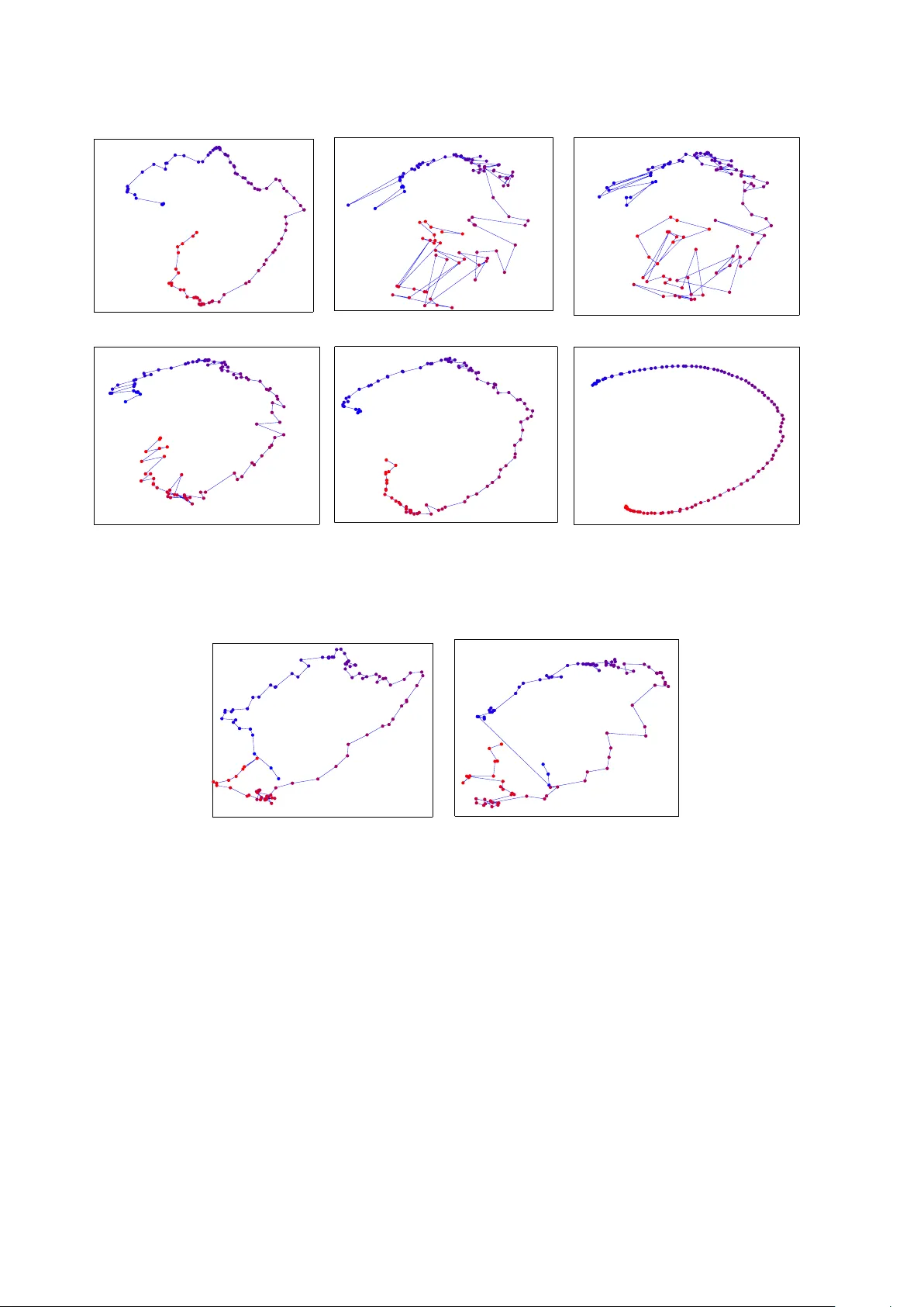
1 Out-of-Sample Extension for Dimensionality Reduction of Noisy T ime Series Hamid Dadkhah i, Marco F . Duarte, Senior Member , IEEE , and Benjamin M. Marlin Abstract —This paper proposes an out-of-sample extension framewor k fo r a global manifold lear ning algorithm (Isomap) that uses temporal inf ormation in out-of-sample points in order to make the embedding more robust to noise and artifacts. Giv en a set of n oise-free training data and its embedding, the proposed framew ork extends the embedding fo r a n oisy time series. This is achieved by adding a spatio- temporal compactness t erm to the optimization objective of the embed ding. T o th e best of our kn owledge, this is the fi rst method fo r out - of-sample extension of mani fold embeddings that lev erages timing informa tion av ailable fo r the extension set. Experimental results demonstrate that our ou t - of-sample extension algorithm renders a more robust and accurate embedding of sequentially ordered image data in the presence of various noise and artifacts when compared to other timing- aware embed dings. Ad ditionally , we show that an out -of- sample extension framew ork based on the proposed algorithm outperform s t he state of the art in eye-gaze estimation. Index T erms —Manifold learning, dimensionality reduction, time series, out-of-sample extension I . I N T RO D U C T I O N Recent advances in sensing technology ha ve enabled a massiv e in crease in the d imensionality o f da ta cap tured from digital sensing systems. Natur ally , the high dim e n sion- ality of the data af fects various stages of the system, from acquisition to processing an d an alysis of the da ta. T o meet commun ication, computation , and storag e con straints, in many applications o ne seeks a low-dimensional emb edding of the high -dimension al d ata tha t shrin k s the size of the data repr esentation while retaining the inf o rmation we are interested in captu ring. This pr oblem of d imensionality r eduction has attracted significant atten tion in the signal processing a nd m achine lear ning communities. The traditio n al metho d f or dimensiona lity reductio n is principal co mponen t an a lysis (PCA) [2], which success- fully cap tu res the structur e of data sets that are well ap proxi- mated by a lin ear subspace. Howe ver , in many application s, the data can b e best mo deled by a no nlinear m a nifold whose geo m etry cannot b e capture d b y PCA. Manifolds This work wa s partially supported by the National Science Founda tion under grants IIS-1239341, IIS-1319585, and IIS-1350522. A portion of this work appeared at the IEEE Internat ional W orkshop on Machine Learning for Signal Processing, 2015 [1]. H. Dadkhahi is with the Electrica l and Computer Engineer ing (ECE) Department and the Colle ge of Information and Computer Sci- ences (CICS), Univ ersity of Massachuset ts, Amherst. E-mail: hdad- khahi@c s.umass.edu. M. F . Duarte is with the ECE Department, Uni- versit y of Massachu setts, Amherst, Email: mduarte@ec s.umass.edu. B. Marlin is with CICS, Univ ersit y of Massachuse tts, Amherst, E-mail: marlin@cs.umass.edu. are low-dimensional geome tr ic stru c tu res that r e side in a high-d imensional ambie n t spac e despite possessing mer ely a fe w degrees o f fr eedom. M anifold m odels ar e a go od match for datasets associated with a phy sical system or ev ent governed by a f ew con tinuous-valued p a rameters. Once th e man ifold mode l is f o rmulated , any poin t on the m a nifold can be essentially repr esented by a low- dimensiona l vector . Ma nifold learn ing me thods aim to ob- tain a suitable nonlinear embedding in to a low-dimen sional space that pr eserves the local structur e pr esent in the high er- dimensiona l d ata in order to simplify data visualizatio n and exploratory data analysis. Examples of man ifold learning methods include Iso m ap [3] , locally linear em beddin g [ 4], Laplacian eigenmaps [ 5], and Hessian eigenmap s [ 6]. All the afo remention ed dimension ality redu ction meth- ods a ssume that the data po ints are stationary and in- depend ent. Howe ver , in m any real-world application s in vision an d imag ing we encounter time series data. In rece n t years, se veral attempts have been made to take advantage of tempor a l infor mation of the data in ord er to discover th e dynamics u n derlying the m anifold. Sp atio-tempo ral Isomap (ST -Isomap) [ 7] empirica lly alters the original weig hts in th e graph o f local n eighbo rs to emphasize similarities among tempo rally rela ted points. Similarly , the temp oral Laplacian eigenma p [8] incorporates tempo ral in formatio n into the Laplacian eigenmap (LE) framew ork. Furtherm o re, [9] extends the g lo bal coor dination mod el of [10] to a dy- namic Bay esian network ( DBN) b y ad ding links among the intrinsic c o ordina te s to accoun t for temp oral depend ency . I n addition, [1 1] applies a semi-supervised regression mod el to learn a non linear mappin g from temporal d ata. Finally , temporal infor mation h as b een similarly u sed in other image proce ssing tasks to improve lear ning perform ance, e.g., [1 2], and its u se is natural when p rocessing video sequences. When the d ata to be embedd ed correspo nds to a time series, all th ese tem poral frameworks of dimen sionality reduction gene rate better quality embedd ed spac es than the initial approach es in the sense that the embedding in dicates the dynamics of the da ta. Howe ver, all o f the mentione d methods ar e designed o nly fo r a given set of tr aining po ints, with no straightfor ward extension of th ese timing- aware embedd in gs f or o ut-of-sam ple p oints. On the o ther h and, many of these dimension ality re- duction algo r ithms (and Isom ap in particular) are sensitive to noise and ar tifacts [13]. This is not de sira b le f or real- world app lications since the data are usually contaminated with noise and various artifacts due to imperf ect sensors or 2 human mistakes. T his sensiti vity is particular ly relevant for emerging arc hitectures for very low p ower sensing, wh ich are subject to increased p resence of n oise and artifacts [14]. In this paper, w e address th e problem of out-of- sample extension of non linear manifo ld embed dings for the specific case wher e the p oints to be extende d co rrespon d to a time series. The aim is to use the sequential ord ering of th e data points to improve th e resilience o f the em bedding o f ou t- of-sample points to various no ise and ar tifact mod els. This improvement is achieved b y enforcing a com pactness for pairs of p oints within a tem poral n eighbor hood window . Our fo c us in this pa per is on Iso m ap for th e sake of concreten ess, but our f o rmulation is generic eno ugh th at it can also be applied to additional nonlin e ar manifold learning algorithm s that a r e fo rmulated as op timization problem s. The contributions of this paper can be summarized as follows. W e propo se an optimiza tio n pro b lem for out- of-sample manifo ld extension with a cost fun ction tha t incorpo rates two distinct terms. The role of the first term is to preserve the m a nifold structure using only th e spatial in - formation fr o m all data points (original and out-of-sample ) . The second term , refer r ed to as spatio-temp oral c o mpact- ness, aims to leverage tempo ral infor mation among out- of-sample points. The comp actness term is defin e d based on a weighted Laplacian for the temporal neighborh ood graph of the o ut-of- sam ple p oints. The use of temporal informa tio n is suitable when processing sequences of data points that correspon d to the traversal of contin u ous path s in the ma n ifold, wh ich is comm only ob served in v ideo sequences whose frame s tra verse paths in image manif olds. Similarly , our use of temporal info rmation in out-of-sam ple extension is m otiv ated by the application of manifold mod- eling of vid eo seq uence frames, where a re ference manifo ld is lear n ed from a clean d ata set. Existing metho ds that aim to leverage spatio-tem poral inf ormation in manifo ld learning are not compatible with this app lication d ue to the lack of tempo ral in formation o n th e referen ce/clean data set. W e showcase the benefit o f leveraging spatio-tem poral informa tio n for out-o f-sample extension by demonstrating higher resilience to the presen ce of noise and distortion in the points inv olved in the extension . T o the be st of our k nowledge, the idea of introdu c ing the spatio - temporal compactn e ss for ma nifold models, its particular setup fo r the o ut-of-sam ple extension proble m , a n d the pro posed optimization formu lation to solve the latter proble m , are novel to o u r work. The application scenario of our p roposed sch eme is as follows. In a train ing stage for nonlinear m anifold lear n ing, we have fu ll control of the environment, which enables us to capture noise-fr e e data. W e then use the captur ed training data to learn the und erlying man if old. In the testing stage (which correspo nds to the no rmal op eration o f th e sensors), we capture data points of lower qua lity , possibly contaminate d with different artifacts/noise patterns, in a sequential order (i.e., as a time series). W e then extend the original nonlinear m anifold em beddin g to the n ewly acquired (noisy) samp les using ou r p roposed alg orithm while le veraging their timing information . The rest of this paper is organ ized as fo llows. W e first revie w the literature on manif o ld lear ning, in particular Isomap, and its spatio-tem poral, denoising, and o ut-of- sample extensions in Section II. In Section III, we derive a framework for out-of- sample extension of Isomap in which tem poral informatio n of the data points is taken into a c count. Experim ental results on a rea l- world dataset is p resented in Sectio n IV. W e conclud e this pap er with discussions o n the propo sed algo rithm and future work in Section V I. W e also summ arize key notation used throug h the paper in T able I. I I . B AC K G RO U N D A. Manifold Models a nd Manifold Learnin g A set of data po ints U = { u 1 , u 2 , . . . , u n } in a high - dimensiona l ambient space R d that have been generated by a n event featu ring m degrees of freedo m co rrespon d to a samp ling of an m -dim ensional manifold M ⊂ R d . Giv en the hig h-dimen sional dataset U , we would like to find the param eterization that has g enerated the manif old. One way to discover this pa rametrization is to embed th e high- dimensiona l data on the m anifold to a low-dimension a l space R m so that th e local geometry o f the manifold is preserved. Dimensiona lity r ed uction meth o ds are devised so as to pre ser ve such geo metry , which is measu red by a neighbo rhood -preserving criteria that varies dep ending on the specific algo rithm. Principal compone n t analysis ( PCA) is perh a ps the most popular schem e for linear d imensionality reduction of high - dimensiona l data [2]. PCA is defined as the o rthogo nal projection of th e data onto a linear subsp ace o f lower dimension m such that the variance o f the pro jected d ata is maximized. Un fortun ately , PCA fails to preser ve the geometric structure of a no nlinear manifold , i.e., a manifold where the mapping from parameters to data is nonlinea r . Sev eral nonlinear ma nifold learning methods can success- fully embed the data into a low-dimension al model wh ile preserving such local g eometry in order to simp lify the parameter estimation pr ocess. B. Isomap For nonlinear manifold learnin g , th is paper fo cuses on the Isomap algorith m, which aims to pr eserve the pairwise geodesic distanc es between data points [ 3]. Th e geod esic distance is defined as the leng th of the shortest path be twe en two data points u i and u j ( u i , u j ∈ M ) alon g the surface o f the manifold M and is d enoted by d G ( u i , u j ) . Isomap fir st finds an app roximatio n to the geod esic distances between each p air of data p oints in a sampling of th e manif old U by constructin g a n eighbor hood graph in which each point is conn ected only to its k n e a rest neighbor s; the ed ge weights are equal to th e cor respond ing pair wise d istances. For neighb oring pairs of data p oints, the E uclidean distan ce provides a good appr oximation for the geod esic distance, i.e., d G ( u i , u j ) ≈ k u i − u j k 2 for u j ∈ N k ( u i ) , (1) 3 T ABLE I: List of important no tations. Notatio n Descripti on Nota tion Descripti on U set of training point s n cardina lity of U L embedding set for training points U N cardina lity of Y Y set of out-of-sample point s m dimensiona lity of L (and X ) X embedding set for ext ension points Y K number of temporal neighbo rs in T T K temporal graph for Y α decay parameter for weigh ting function ∆ n squared dista nces betwe en training points U λ regul ariza tion paramete r ∆ X squared dista nces between training points U and e xtension point s Y ω temporal weighting function where N k ( u i ) d esignates th e set of k nea rest neig hbors in U to th e point u i ∈ U . For non-n e ighbor in g po ints, the geodesic distance is estimated as the length of the sho rtest path along the n eighbor hood graph, which can be found via Dijkstra’ s algorithm . Then, multidime n sional scaling (MDS) [15] is applied to the resulting g eodesic distan c e matrix to find a set of low-dimension al points that best match such distance s. C. Out-o f- Sample Extension for I somap Out-of-sam ple extension (OoSE) gene r alizes the result of the non lin ear manifold embedd ing f or new data points. Sup- pose we have n trainin g data po ints U = { u 1 , u 2 , . . . , u n } . The embe dding L = { ℓ 1 , ℓ 2 , . . . , ℓ n } of the training po ints is obtain ed by ap plying MDS to the g eodesic distan ce matrix o f the n tr aining poin ts. More p recisely , the cen- tralized squar ed geodesic distances can be obtained as ∆ c = − 1 2 H n ∆ n H n , where ∆ n is the matrix of squar ed geodesic distances (i.e., ∆ n [ i, j ] = d 2 G ( u i , u j ) ) and H n is the centering matrix defined by the form ula H n [ i, j ] = δ ij − 1 n . Th e n , the m -d imensional embed ding L for the n training poin ts U = { u 1 , u 2 , . . . , u n } is given as the columns o f the matr ix L =      √ λ 1 · v T 1 √ λ 2 · v T 2 . . . √ λ m · v T m      , where λ i and v i are the eigenv alues an d eigenvectors of th e centralized squ ared geode sic d istance matr ix ∆ c , respectively . T o o btain the extension of the embeddin g L to the o ut-of- sample (testing) set Y = { y 1 , y 2 , . . . , y N } , let ∆ X denote the n × N matrix of squared geod esic distances between the N out-of - sample (testing) points Y and th e n tra ining points U ; these g eodesic distances are estimated as before with an augmen ted graph includin g links to th e k n earest neighbo rs of each out o f sample p oint. The out-of- sample extension X = { x 1 , x 2 , . . . , x N } o f the embe d ding L to the p oints Y is given b y the columns of the m a trix [16], [17] X = 1 2 L # ( ¯ ∆ n 1 T N − ∆ X ) , (2) where 1 N denotes an all-ones vector of length N , ¯ ∆ n is the c olumn mean of ∆ n , i.e. , ¯ ∆ n = 1 n ∆ n 1 n , an d L # is the pseudo-inverse transpose of L , given by L # = ( L T ) † =      v T 1 / √ λ 1 v T 2 / √ λ 2 . . . v T m / √ λ m      . Note th at, to the best of our knowledge, the literature on out-of-samp le extension do es no t exploit the sequential orderin g of data to mitigate th e p ossibility o f embeddin g errors due to the presence of noisy and contaminated data. D. Spatio- T emporal Isomap In Isomap, the neig h horho od grap h is formed b y linkin g each p oint in U to its k - nearest n eighbo r s in th e same set. S patio-T emporal Isoma p (ST -Isomap) leverages se- quence/timin g informatio n { ( u i , t i ) } present for each of the training points u i ∈ U . ST -Isom ap ap pends ed ges betwe e n pairs of adjacent temp oral neighbo rs ( A TN), i.e., pa ir s o f immediate tempo ral n eighbo rs whe re t j = t i ± 1 , to the neighbo rhood grap h . The weights (i.e., d istances) b etween A TNs are scaled down by a factor giv en by the constant parameter c AT N , which is used to emph asize the correlation between a p oint a nd its adjacen t tempo ral neigh bors. ST -Isomap also mo difies the grap h weig hts of a sub set of the k - nearest neighb ors of each point that satisfy certain spatio-tempo ral conditio ns. First, the set of points in a tem- poral wind ow of size ǫ a r ound each po int u i is conside r ed as its trivial matches , den oted by T ǫ ( u i ) . Suppose that the point u j ∈ T ǫ ( u i ) is the closest trivial match to p oint u i , i.e., d G ( u i , u j ) = min u k ∈T ǫ ( u i ) d G ( u i , u k ) . Now , the subset of k -near est neighbo rs with distances less than or equal to d G ( u i , u j ) from u i are considered as non-trivial matches and the resu lting set is re f erred to as common temp oral neigh bors ( CTN): CTN( u i ) = { u j ∈ U : u j ∈ N k ( u i ) , d G ( u i , u j ) ≤ min u k ∈T ǫ ( u i ) d G ( u i , u k ) } . In oth er words, CTN are a subset of the (sp atial) n earest neighbo r g r aph, consisting of p o ints which are sp atially closer to a given p o int than its closest temp oral neighb or (i.e. the closest tr ivial match) . I n a sense, CTN are u sed to ide n tify data p oints in the local sp atial neig h borho od of each po int u i that are more likely to be analogou s to u i . Finally , the constan t parame te r c C T N is used to emph asize 4 the similarity between ea c h p oint and its CTN set via reducing the corr e sponding weights by a scaling factor of c C T N . Note that ST -Isom ap is devised to better un cover the spatio-tempo ral stru cture u nderlyin g th e manif old data, rather than to faithfully recover the embe d ding of d ata contaminate d by noise o r artifact models. In add ition, ST - Isomap doe s not address the ou t-of-sample extension prob- lem. Nonetheless, we form ulate a straightforward ad apta- tion of out-o f -sample extension from Isomap to ST -Isomap in Section IV. E. Manifold Denoising The major ity o f the literatur e o n manifold models fo r noisy data fo cuses on a given set o f noisy training data, aiming at red ucing the error of th e re c overed data p oints in the amb ien t space rath er th an the embedd ed trajector y . In [18] a prepro cessing proced ure is proposed that e n ables Isomap and LLE algo r ithms to ach iev e mo re robust recon- struction of n o nlinear manifolds in the presence of Ga u ssian noise. Th is is achieved by comb ining locally smo othed values of data po ints, whic h are in tu rn computed via the so-called linear error-in-variables mo del of local structure. [19] tackles the same prob lem in Laplacian eig enmaps by reversing the diffusion pr ocess employed therein. This is done by approxima tin g th e generator o f the diffusion process by the graph Laplacian of a rando m neig h borho od graph. [20] p roposes a m a n ifold denoising algorith m based on Gaussian process latent variable models (GPL VM) to handle data contam inated by Gaussian and salt-and- pepper noise. GPL VM u ses th e maximum a posteriori estimate o f the tr ansformatio n m atrix in the la te n t variable mode l to map the latent variables back to the d ata spa c e. In [ 21], the authors introduce Locally Lin ear De n oising (LL D), an algorithm tha t appro ximates m anifolds with locally linear patches by constructin g n earest neighb or graphs. Each point is then lo c a lly denoised within its n e ig hborh ood. The latter algorithm h a s been used in denoising o f images in the am- bient space and improves the p erform a nce of classification in the embedd ed sp ace in the presen ce of salt-and-pep per, Gaussian, m otion blur, and occlusion a r tifacts. In [2 2], a preprocessing pro cedure, ca lled Manif old Blurring Mean Shift (MBMS), is propo sed for deno ising manifold data based o n b lurring mean-shif t updates. Each iteration of the MBMS algor ithm h as two steps. T he first step is a blurr in g mean-shif t update that moves data po ints to the kern el a verage of their neigh bors with a Gaussian kernel of width σ . Then, a pro jectiv e step is computed using the local PCA of dimensiona lity L on the k neare st neighbo rs o f each po int. Note that none of the mentioned alg orithms take advan- tage of tempor al info rmation among the images. Moreover , none of th ese algorithm s addr ess the out-o f-sample exten- sion p roblem in the presence of noise and artifacts. I I I . M A N I F O L D E X T E N S I O N F O R T I M E S E R I E S In th is section, we describ e the formulation of a new algorithm for out-o f-sample extension of Isomap non linear manifold em bedding s that also aim s to lev erage tempo ral informa tio n in or der to improve the quality of the em bed- ding of no isy an d co rrupted data time series. Recall that the embed ding of o ut-of-sam ple points is given b y the matrix equation (2). Alterna ti vely , the em- bedding X = { x 1 , x 2 , . . . , x N } of out- of-sample poin ts Y = { y 1 , y 2 , . . . , y N } can be expressed as the solution to the following optimization pr oblem: X = a rg min X     1 2  ¯ ∆ n 1 T N − ∆ X  − L T X     2 F , (3) where k . k F denotes the Frob enius matrix norm, a n d the columns o f the matrix X correspon d with the emb e d dings in X . In o ur problem setup, we a ssum e that the o u t-of- sample poin ts { y 1 , y 2 , . . . , y N } have bee n sampled at time instances { t 1 , t 2 , . . . , t N } , r espectively . T o characterize th e spatio-temporal similarity , we first define the spatio-tempo ral compa c tness functio n C ω ( Y , τ ) of geod esic distances and temp oral informatio n for th e time series: C ω ( Y , τ ) : = N X i =1 X y j ∈T K ( y i ) d 2 G ( y i , y j ) · ω ( τ ij ) , (4) where ω is a temporal weighting fu n ction, τ i,j = | t i − t j | , and T K ( y i ) is the set of K n earest temp oral neighb ors to point y i in Y : T K ( y i ) = { y j : j ∈ N , max { 0 , i − ⌊ K / 2 ⌋ } ≤ j ≤ min { i + ⌊ K/ 2 ⌋ , N }} . Note th a t K 6 = k from ( 1) in general, and there could be many choic e s f or the temporal weighting fu nction. One suc h choic e is the expone n tial decay fu nction ω ( τ ij ) = exp( − α · τ ij ) with a deca y parameter of α . This choice of the weighting f unction is natural sinc e the distance of each p oint to its immed iate temporal neighb ors is mor e likely to b e small an d this likelihood d ecreases g radually as we consider subsequent temporal n eighbo rs. W e assume that the geodesic d istances in the am bient space of eac h tempor al n e ighbor h ood of the o ut-of- sam ple data points should be small so that the compactness term in (4) is also small. W e aim to incorpo r ate this com pactness in th e embe d ding framework. This can be ach iev ed by lev eraging the fact tha t the Eu clidean distances in the embedd in g space are matched to their g eodesic counter p arts in th e ambient space. Therefo re, we m odify the expression for the co m pactness b y leveraging the expected relation sh ip between th e or iginal geo desic distances for Y and th e Euclidean distances o f th e embedd ed data points X : d 2 G ( y i , y j ) ≈ k x i − x j k 2 2 = Tr ( B ij X T X ) , where B ij is an all zeros matrix of size N × N excep t for four elements, B ij [ i, i ] = B ij [ j, j ] = 1 and B ij [ i, j ] = B ij [ j, i ] = − 1 . The comp actness term in (4) can then b e reformu lated as C ω ( X, τ ) = N X i =1 X y j ∈T K ( y i )  T r ( B ij X T X ) · ω ij  , 5 where ω ij = ω ( τ ij ) . In order to incorpor ate the tempora l info rmation am ong the sequence of out-o f-sample points, we in tr oduce the spatio-tempo ral compactn ess constraint to the optimization as f ollows: X = arg min X     1 2  ¯ ∆ n 1 T N − ∆ X  − L T X     2 F (5) subject to : C ω ( X, τ ) < µ, where C ω ( X, τ ) is the sp atio-tempo ral comp actness amon g out-of- sample poin ts and µ is a constant. In word s, we would like the spatio-temp oral compactness among suc- cessi ve po ints to be less than a constant µ in order to lev erage the tempor al informatio n of da ta p oints in d eriving the embeddin g. Note th a t we can rewrite the compactn ess as f ollows: C ω ( X, τ ) = T r   N X i =1 X y j ∈T K ( y i ) ω ij B ij X T X   = Tr  AX T X  , (6) where the matrix A is gi ven by A = N X i =1 X y j ∈T K ( y i ) ω ij B ij . Note that we can alternatively view A as th e Laplacian matrix for a weigh ted tempo r al neighb orhoo d graph. Letting Q = 1 2 ( ¯ ∆ n 1 T N − ∆ X ) , the optimizatio n in ( 5) becomes X = arg min X k Q − L T X k 2 F (7) subject to : C ω ( X, τ ) < µ. W e can r ewrite the optimizatio n in (7) using a Lag rangian relaxation ( λ > 0) in the following way: X = a rg min X k Q − L T X k 2 F + λ · C ω ( X, τ ) . (8) Note th at k A k 2 F = Tr ( A T A ) , where Tr ( . ) represents the trace operator . Hence, the first term of the optimization in (8) can be written as k Q − L T X k 2 F = Tr (( Q − L T X ) T ( Q − L T X )) . (9) Plugging C ω ( X, τ ) and k Q − L T X k 2 F from Equations (6) and (9) into the o ptimization in (8) yields X = a rg min X T r  ( Q − L T X ) T ( Q − L T X )  + λ · T r ( AX T X ) = arg min X T r  Q T Q − 2 Q T L T X + X T LL T X  + λ · T r ( AX T X ) ( a ) = a rg min X T r  − 2 Q T L T X + X T LL T X  + λ · T r ( AX T X ) = arg min X T r  C T X  + T r  D X X T  + λ · T r  AX T X  , (10) Algorithm 1 Manifo ld Exten sion fo r Time Series (MET S) Inputs: Embedd in g L for training points U , param eters K and α , regularization p arameter λ , tem poral neigh - borho od graph T K for extension set, squared distances ∆ X between training p oints U an d extensio n points Y , squared d istances ∆ n between training po ints U Outputs: Embedd in g X f or Y Initialize: A ← 0 N × N for i = 1 → N do for j ∈ T K ( y i ) do B ij ← 0 N × N B ij [ i, i ] ← 1 , B ij [ j, j ] ← 1 B ij [ i, j ] ← − 1 , B ij [ j, i ] ← − 1 ω ij ← exp( − α · τ ij ) A ← A + ω ij B ij { Constructing weighted Laplacian matrix A fo r tempo r al neighb orhoo d grap h T K } end for end for D ← LL T Q ← 1 2 ( ¯ ∆ n 1 T N − ∆ X ) C ← − 2 LQ vect ( X ) ← − 1 2  ( I ⊗ D ) + λ · ( A T ⊗ I )  − 1 · vect ( C ) X = { x 1 , x 2 , . . . , x N } { x i is th e i -th co lumn of X } return X where in ( a ) th e co nstant matr ix Q T Q h as be e n dro pped from the objective function. No te th at we d enote C = − 2 LQ and D = LL T . Additiona lly , we note that T r  X T D X  = T r  D X X T  due to in variance o f trace under cyclic permutation s. Next, we denote the objective function in (1 0) by J , and take the deriv a ti ve of J with respect to the embedd ing matrix X as follows: ∂ J ∂ X = C + ( D + D T ) X + λ · X ( A + A T ) ( b ) = C + 2 D X + 2 λX A, (11) where ( b ) is due to the matrices D and A bein g symm etric. Solving ∂ J ∂ X = 0 for X g ives us the so lu tion to th e optimization in (1 0), whe re 0 is an all-zeros m a tr ix of size N × m . In o rder to solve the ma tr ix equa tio n ∂ J ∂ X = 0 , we use the Kro necker p roduct and the vectorized format of each te r m: vect  ∂ J ∂ X  = vect ( C + 2 D X + 2 λX A ) = vect ( C ) + 2 ( I ⊗ D ) vect ( X ) + 2 λ ( A T ⊗ I ) vect ( X ) , (12) where ⊗ d esignates the Kr onecker pr o duct op erator an d I is the id entity matrix. Setting ( 12) equal to zero an d solving for vect ( X ) yields: vect ( X ) = − 1 2  ( I ⊗ D ) + λ · ( A T ⊗ I )  − 1 · vect ( C ) , (13) which pr ovid es the embe d ding obtained fro m the solutio n to (5). For brevity , we refer to the proposed algorithm as 6 manifold extension for time series ( METS), a summary of which is presen ted in Algorithm 1. Note th at Eq uation (13) involv es a m atrix inversion. Considering that ra nk ( A 1 ⊗ A 2 ) = ra n k ( A 1 ) × rank ( A 2 ) , analysis of the r ank of th e first and second terms in the matrix under in version boils d own to tha t of D an d A , respectively . The matrix D is inv ertible since th e rows of L are orth onorm a l. Since A is a weighted Laplacian matrix, it is of r a n k N − 1 with the all-o nes vector being the eigenv ector cor r espondin g to th e zero eigen value. Howev er , the sum of I ⊗ D and A T ⊗ I is full rank un less we have a pathological data structur e. Note also that th e complexity of (13) is O (max { nmN , ( mN ) ǫ } ) , where O (( mN ) ǫ ) is the complexity of matrix inversion fo r an mN × mN matrix. In compar ison, the comp lexity of Iso map Oo SE from Equation (2) is O ( nmN ) . Hence, as long as the number of training data points n is sufficiently large, co mpared to m and N , the co mplexity o f METS matches that of Isomap OoSE. Note that the above-mentione d computatio n al complexities do n ot include the comp u tation of the geodesic distances. I V . N U M E R I C A L E X P E R I M E N T S : O U T - O F - S A M P L E E X T E N S I O N O F T I M E S E R I E S In th is section we inves tigate the robustness of the propo sed algorithm to different types of artifacts. In all the experiments, we conside r image manifold datasets, wher e each d ata p oint corr esponds with an im age. W e start f rom a dataset of origin al imag es that we treat as “ clean” im ages, and we synthe size noisy images b y ad ding several types of noise a n d artifacts to them. W e consider thre e types of noise and artifacts: salt-and- pepper n o ise, Gaussian noise imposed on the pixel intensities, and motion blu r ring as caused by camera movements. Algo rithms tha t are resilient to different noise/artifact types ar e high ly d esirable in practice as inferrin g noise types is often challeng ing. For our exper im ents, we con sider two da tasets: the eyeglasses dataset [14] an d the Statue dataset [ 23]. The eyeglasses dataset is a custom eye-track ing dataset of 11 1 × 11 2 -pixel c a ptures from a co mputation al eye- glasses pro totype. The p rototyp e featu res low-power cam- eras mounted on a pair of eyeglasses th at a re trained on the user’ s eyes, with the goal of tracking the g aze location of the user over time. Th e dataset contains n + N = 900 + 100 images and the dim ensionality of the learn e d m anifold is m = 2 . A uniform sequential ordering exists among the N out-of -sample po ints. A subset of consecutive out- of-sample points is shown in Figure 1a. Ex ample noisy images with the three types o f artifacts under study are also depicted in Figure 2. The Statu e d ataset con sists of 94 4 images of a rigid object on a turntable platfor m captured f rom a camera o n an elev ating ar m. T he imag e s are captu r ed every 6 degree s of rotation from 6 to 354 degrees an d every 6 degre es of elev ation f rom 0 to 90 d egrees. Each imag e is cr opped and resized to 128 × 128 . In ou r experiments, we u se ha lf o f the ima ges at o ne of th e elevation levels as out-o f-sample points (i.e., N = 29 successive rotations in that elev atio n lev el form the ou t-of-samp le poin ts) and use the re maining points ( n = 9 15 ) as training data. Note th a t this situation represents a pr a ctical scenario since we are testing over a missing slice of the m anifold co rrespon ding to th e rotatio ns in an e lev ation le vel of the camera. Sample im ages from the Statue dataset are shown in Figure 1b. The exper im ents in this sectio n pur sue the fo llowing general framework. First, we obtain the Isomap emb edding for n train in g points. Next, we obtain th e OoSE of both clean and noisy N out-of- sample poin ts. Th e OoSE of clean po ints is conside red as a reference for per f ormance measure, and we would like the embed ding of the no isy version of the out-of-sam ple p oints to b e as close to that of the clean d a ta as possible. W e set k = 20 in a ll th e experiments fo r bo th th e eyeglasses and Statue datasets. For each value of the no ise pa r ameter, we gener ate 6 instan c e s of n oise. W e use the first instance of n oise to find the best-perfo rming value of the param eter λ by a gr id sear ch. The selected value o f λ ( which is different in gener al for different noise parame te r s) is used to me asure the perfor m ance o f th e prop osed algorithm on the rem aining instances of no ise. Finally , we average the error over the latter instances. Note that f or Isomap we cannot dir ectly co mpare the two sets of o u t-of-samp le poin ts [24], as the embed dings learned from different samplings of the manifo ld are often su b ject to tran slation, rotation, and scaling. Th e se variations mu st be ad dressed via manifold align ment before the embedd ed points a r e compared . W e find the o ptimal alig nment of the clean and noisy embeddin gs via Pr ocrustes ana lysis [25], [26] and apply the re su lting tr anslational, rotational, and scaling compon ents on the OoSE points. Finally , we measure the OoSE erro r E a s th e average ℓ 2 distance between matching points in the two embe ddings, i.e., out- of-sample extension of aligned clean and denoised testing data: E = 1 N N X i =1 k z i − w i k 2 , where Z = { z 1 , z 2 , . . . , z N } is the o u t-of-samp le ex- tension o f clean data via Isomap OoSE, and W = { w 1 , w 2 , . . . , w N } is the OoSE from noisy data for the algorithm under test after alignmen t with Z . W e co mpare the pe rforman ce of th e prop osed algorithm against an adaptation o f Isomap out-of-samp le extension to ST -Isomap. W e n ote tha t we compar ed th e results of the pro posed algorithm with those of ST -Isomap since it can be extend e d to o ut-of- samples in a similar fashion to Isomap OoSE. T o obtain the out-o f-sample extension of ST -Isomap , we find the distances of the o u t-of-samp le points with training points v ia the neighbo rhood graph of the ST -Isomap algo rithm, and then use (2 ) to find the embedd in g f or the out-o f-sample poin ts. Note th a t since Isomap an d ST -Isom a p use d ifferent n eighbor hood graphs regardless o f the p arameter values o f the ST -Isoma p, the embedd in g of clean d ata v ia ST -Isoma p differs from that 7 (a) (b) Fig. 1 : Sample images used for out-of-sample extension. ( a ) Eyeglasses dataset; ev ery second i mage in a sequenc e of 18 successi ve data points, ( b ) Statue dataset; 9 successiv e data points corresponding to successiv e rotations i n an elev ation lev el of the camera. Fig. 2: S ample noisy images from the ey eglasses dataset. Fr om left to right: noise-free, salt-and-pepper noise with p = 0 . 2 , Gaussian noise wit h σ = 0 . 1 , and motion blur with length of 20 pixels and angle of 45 degrees. of I so map. Henc e , we cannot dir ectly co mpare the two embedd in g spaces. Th u s we first a lig n the two OoSE embedd in g spaces, and then ev aluate the error between the aligned embedd in g ob tained via ST -Isomap on clean an d noisy d a ta . W e set the value of the parameter c AT N = 1 as experimentally this selection p roduces the m inimum error . W e then perform a g rid search over the window size ǫ and parame ter c C T N , in a similar manner to the ev aluatio n of the parameter o f the p roposed alg orithm, i.e., using 6 instance s of noise. No te that we are giving an advantage to ST -Isomap o ut-of-sam p le extension over ou r propo sed method by supplyin g tempora l inf ormation abou t both training an d out-o f-sample poin ts to the algorithm. As mentioned in Section II, the algorithms on manifold denoising fail to add ress the out-of -sample extension prob- lem. In ad dition, non e of the mentione d algorith ms take advantage of temp oral information am ong the images. In order to make a fair comparison with manifold deno ising algorithms (as b a selines), we apply manifold d enoising algorithms on the collectio n of both training and o ut-of- sample p oints, and compar e the em beddin g for the de noised version of ou t-of-samp le p oints with that of th e clean d ata. Since th e manifo ld denoising algorithm s take ad vantage of the neigh boring points to ob tain th e denoised version of each p oint, the inc lusion of clean poin ts dur ing den o ising improves the quality of denoising fo r the (noisy ) o ut-of- sample p oints. W e consider M BMS, which is one o f th e mo st recen t algorithms for den oising of man ifolds. W e also con sidered LLD, an alternative manifo ld den o ising algorithm, b ut in our exper im ents it turned out to be less resilient to noise. Specifically , for the ran ge o f no ise le vels that we consider in our experimen ts, LLD failed to p erform well and the embedd in g of the resulting denoised po in ts was c omparab le to that of the noisy poin ts. This can be associated with the n eighbo rhood selection mechanism emp loyed in LLD where, f or each po int, the set of points th a t inclu de that point in their neighborh ood is c o nsidered d uring denoising. Since at higher noise levels the majo r ity of n eighbor hoods for clean p o ints is comp o sed of oth er clean poin ts, the noisy po ints mostly belo ng to th e neig hborh oods of noisy points. Hence, the denoised version o f the noisy point is not an improvement over th e noisy point. In co ntrast, the MBMS algorithm de noises eac h poin t by consider ing its neighbo ring points, i.e., MBMS con siders neig h bors in the opposite d ir ection to that o f LLD. It turns ou t that the neighbo rhood of a noisy point in cludes a majority o f cle a n points and a mino r ity o f n oisy points. Hence, the de noised version of that po int is a major improvement over the counterp art noisy version. As such, we d o not consider LL D and only in clude MBMS in our experimental results. For MBMS, we set the value of th e parameters L = 1 or L = 2 (whichever pr ovides the b est per forman ce) and the n umber of iterations to 3 , as suggested by the au th ors; our experiments also confirms that this settin g produ ces the best result. In order to choo se the value of the para m eter σ , we p erform a g rid search over the inter val [1 , 20] on the first instance of noise, ev aluate the alg o rithm with the chosen value of σ on the remain ing in stances, and repo rt the av erage erro r . A. Salt-a n d-P epp er Noise W e co nsider salt-and -pepp e r noise where th e inten sity of each pixel is rando mly flip ped with a probability of p 8 to either zero or on e, with both having eq ual proba b ility p 2 . W e vary p fr o m 0 . 2 to 0 . 6 with a step size of 0 . 1 . For the eyeglasses dataset, the selected values f o r the parameter λ are [0 . 02 , 0 . 14 , 0 . 2 , 0 . 53 , 9 . 0] × 10 5 , respectively . Figu re 4a co mpares the perfor mance o f the proposed algor ithm at different noise le vels against that of Isom a p OoSE, ST - Isomap Oo SE, and MBMS, for th e eyeglasses dataset. As can be o bserved from this fig u re, th e average ℓ 2 -norm e r ror of the prop o sed algo r ithm is lower than those of Isomap OoSE a nd ST -Isomap OoSE. The error bars indicate th e variability over the five noisy instance s of the out-of - sample points via the standard error of the mean (SE M ). Note that SEM is compute d as s √ 5 , where s is the sample standar d deviation. W e c a n ob serve fro m the plots that th e variability of all the algor ithms, specifically METS, is qu ite small for both salt-an d-pep per and G a u ssian noises. W e see a higher variability for the mo tion blur artifact expe riments, which is to be expe c ted since the latter artifact m odel is n ot zero - mean and ha s a higher variation over the pixels (du e to rotations). Recall that METS incorpo rates two p arameters: neigh- borho od size K of the temporal g r aph and decay parameter α of the tim e weighting function . Figure 3 demo nstrates the perfor m ance of METS at different values o f the parameters K and α for a time series con taminated by a n instance of salt and p epper noise with p = 0 . 4 . As we can see from this figure, METS achieves its best perfo rmance over a large range of the pa r ameters K and α . Intu itiv ely , either K or α ca n be leveraged to set th e level o f depen dence among th e temporal n eighbor s in the emb edding space. Experime n tally , the observed pattern tur ned out to be similar at different no ise lev els; hence the values o f the optimal parameters K and α are fairly ro bust to no ise level and are merely d ata depend ent. Finally , we note that other choices for the weightin g func tio n are possible, an d the perfor m ance of METS tu rned out no t to b e sensitiv e to the cho ice of th e we ig hting fun ction. As an example, we also tried a Gaussian kern el for the weighting function , and o btained virtually identical re sults to those for th e exponential decay kern el. Intuitively , the Gau ssian kernel behaves very similar to the expone n tial deca y fu nction in that it mo dels the decre a se in likelihood fo r th e similarity of the embeddin g of eac h p oint with its subsequent temporal neighbo rs; the only difference is th at the Gaussian functio n s decay with respect to time is faster than that of the exponential fun c tio n. As a rule o f thumb, we may fo llow one of the following procedu res in selection of the parameter s K and α : ( i ) p ick a large value fo r th e pa r ameter K (it can be set to N , in which case we e ssen tially drop the p arameter K from the algorithm) and tun e the value o f the param eter α , or ( ii ) set α to a sm a ll value (it c a n be set to zero, in which case we essentially dro p the par ameter α from the algo rithm) and tune the value of the parameter K . The equivalence of the two p r ocedur e s can be explained as follows. Assume that K 1 is the optimal neig h borho od size in the pro cedure ( i ) , which ind ic a te s the optimal numbe r of tem poral neigh b ors to be inco r porated in the embed ding. Intuitiv ely , the excess α K 0 0.2 0.4 0.6 0.8 2 4 6 8 10 12 14 16 18 20 2.4 2.5 2.6 2.7 2.8 2.9 3 3.1 Fig. 3 : Evalu ation of METS at differe nt va lues for the parameters K and α . of the temporal neighbo rs K 2 > K 1 in procedu r e ( ii ) can be c ompensated by in creasing th e decay parameter α so that the impact of the extra neighb ors is mostly igno red in the embedd ing. Throu ghout the experim ents we follow the second proced ure. For th e eyeglasses d a taset, we set K = 10 an d α = 0 (altern ativ ely , we can set K = 20 and α = 0 . 3 and virtually achieve the same resu lt) . In the exper iments for the Statue d ataset, we set K = 2 and α = 0 . For the Statue dataset, the selected values of th e par am- eter λ for METS ar e [0 . 5 , 1 . 5 , 3 , 9 . 5 , 12 ] × 10 6 at different noise levels. Figu r e 4d comp ares th e performanc e of METS at different noise levels against that o f Isomap OoSE, ST - Isomap OoSE, and MBMS, for the Statue dataset. As we can see from this figure, MBMS only improves the perf o r- mance margin ally over the plain Isom ap OoSE. Moreover , ST -Isomap genrally does not perform well for the Statue dataset. B. Gaussian Noise W e consider Gaussian noise with zer o m e a n an d variance of σ , where we vary σ fro m 0 . 1 to 0 . 5 with the step size of 0 . 1 . When using the eyeglasses dataset, the selected values for the parameter λ are [0 . 25 , 1 . 25 , 1 . 75 , 2 . 0 , 4 . 5] × 10 4 , respectively . Figu r e 4 b compa res the per forman c e of the propo sed algorithm at d ifferent Gaussian noise variance lev els again st that of Isom a p OoSE, ST -Isomap OoSE, and MBMS. Figure 5a dep icts the Isomap trajecto ry for the cle a n out- of-sample poin ts. Its noisy counte r part with the ad dition of an instance of Gaussian noise with p = 0 . 2 is shown in Figur e 5 b. In ea ch plot, seq uentially adjacen t points are connected b y a b lue line and tem poral o rder is color coded fr om blue to red. W e obtained the out-of -sample extension of the noisy d ata by th e pr oposed algorithm with three settings o f the parameter λ ; λ = 0 . 5 × 1 0 4 , 1 . 25 × 10 4 , and 10 × 10 4 as depicted in Figu r es 5d, 5e, 9 0.2 0.3 0.4 0.5 0.6 2 3 4 5 6 7 8 9 10 p Error Isomap OoSE ST−Isomap OoSE MBMS METS (a) 0.1 0.2 0.3 0.4 0.5 2 3 4 5 6 σ Error (b) 10 20 30 40 50 1 2 3 4 5 β Error (c) 0.2 0.3 0.4 0.5 0.6 2 4 6 8 10 p Error Isomap OoSE ST−Isomap OoSE MBMS METS (d) 0.1 0.2 0.3 0.4 0.5 1 2 3 4 5 6 7 8 9 σ Error (e) 10 20 30 40 50 5 10 15 20 β Error (f) Fig. 4: Performance ev aluation for out-of-sample extensio n of t he data points with salt and pepper noise (first column), Gaussian noise (second column), and motion blur artifact (t hird column) for eyeglasses dataset (first row), and S tatue dataset (second ro w). and 5f, respectively . Among the mentioned values of the parameter λ , λ = 1 . 25 × 10 4 produ ces the minimum ℓ 2 - norm error in the rec overed trajectory when co mpared to Isomap tra je c tory for th e clean out-of -sample points. This can be verified by the similarity of the trajector y shown in Figure 5e to tha t of Figur e 5a. As can be observed from th e figu re, a smaller λ overfits the no isy trajectory and retains the noise in th e embeddin g, whereas a larger one oversmooths the trajectory . In creasing the value of the parameter λ eventually converts the embed d ing’ s tr a jectory to an almo st-straight curve. T his is to be expected since ev entually the spatial informatio n will be n eglected and the embedd ing will r etain only the temp oral information of the time serie s. Note that setting λ = 0 in the pro posed algorithm, c o n verts it into the plain Isom a p OoSE and returns the no isy trajecto ry , i.e., Figure 5b. Figure 5c shows the d enoised trajectory obtaine d via MBMS. Figure 6 demonstrates the align e d ST -Isomap OoSE traje c to ry on c lean an d noisy data. W e note that for th e other types o f noise considered in the sequel, th e embedd in gs obtain ed fro m th e d ifferent algo r ithms we test are remin iscent of tho se shown in Figure 5 an d 6, and thus we do no t inclu de th em in this paper . For the Statue dataset, the selected values of the pa- rameter λ are [0 . 1 , 1 . 3 , 2 . 3 , 4 . 4 , 7] × 1 0 6 at different noise lev els. Figure 4e demon strates th e perform a nce of d ifferent algorithms at different n oise levels, wh ich is similar to th o se for the salt and pepper noise fo r the same dataset. C. Motion Blur W e use a lin ear m otion m odel to simulate the motion blur artifact. The ar tifact is applied via co n volution by a filter th a t appro ximates the linear motio n of a c a mera by η pixels, with an angle o f θ degrees in a coun ter clockwise direction. W e consider a uniform distrib ution for θ over the interval [0 ◦ , 360 ◦ ] and a Gamma distribution for η (with PDF of p ( x ) = 1 Γ( α ) β α x α − 1 exp( − x β ) , where Γ( . ) de n otes the G a mma fu nction). W e set th e sha pe para meter of the Gamma PDF α = 1 and vary the scale parameter β from 10 to 50 b y step size of 10 in order to produce d ifferent strengths of m otion blur . The selected values for the param- eter λ ar e [0 . 2 , 1 . 0 , 1 . 3 , 1 . 6 , 2 . 4] × 1 0 4 , r e sp ectiv ely . Figure 4c comp ares the p e r forman ce of the p roposed algorith m at different values of the scale paramete r β again st that of Isomap OoSE, ST -Isom ap OoSE, and MBMS. For the Statue dataset, the following values of the pa- rameter λ are selected when we vary β fr om 10 to 50 , respectively: [0 . 3 , 9 , 11 , 15 , 100] × 10 6 . Figure 4f compar es the perf ormance of d ifferent algorithm s o n the Statue dataset co ntaminated by the motion blur artifact. From the figure, ST -Isomap outpe r forms Iso map OoSE and MBMS at no ise levels above β = 20 . As for other a rtifacts, METS outperf orms Isomap Oo SE, MBMS, an d ST -Isom ap. V . N U M E R I C A L E X P E R I M E N T S : A P P L I C A T I O N I N E Y E G A Z E E S T I M AT I O N Finally , we co nsider an ap p lication of manif o ld mod els in our m otiv ating comp utational eyeglasses pla tf orm. More 10 (a) (b) (c) (d) (e) (f) Fig. 5: Effect of the value of the parameter λ on t he embedding of out-of-sample points for the eyeglasse s dataset. ( a ) Isomap OoSE trajectory for clean data, ( b ) Isomap OoSE trajectory for noisy data with Gaussian noise w i th σ = 0 . 2 , ( c ) OoSE trajectory of data denoised via MBMS, OoSE of noisy data via MET S for ( d ) λ = 0 . 5 × 10 5 ; ( e ) λ = 1 . 25 × 10 5 , and ( f ) λ = 10 × 10 5 , respectiv ely . Fig. 6: ST -Isomap OoSE trajectory of the eyeglasses dataset for ( a ) clean and ( b ) noisy data with G aussian noise with σ = 0 . 2 . precisely , we fo cus on the Eyeglasses dataset, illustrate d in Figure 1a, which is collected fo r the purpo se o f training an estimation algorithm fo r eye ga ze po sition in a 2-D ima ge plane. The dataset corr e sponds to a c o llection of image captures of an eye fr om a camera m ounted on an eyeglass frame as the subject focuses the ir gaze into a dense grid of known positions (size 11 1 × 1 12 , covering a 36 degrees of arc) that is used as ground tru th. T wo p rimary ap proache s has been used in the litera - ture for eye ga z e estimation. In featu r e-b ased app roaches, geometric feature s such as contour s and corner s of the pupil, limbus an d iris, are used to extract fe a tu res of the eye [27], [28]. T he drawback of this appro ach is that it works best with Near-Infrared (NIR) illumination sources, which, through their positionin g relative to the camera, can make the pupil appear brighter or darker, thereby m aking it easier to detect the bo undary [ 14]. When usin g visible light, feature-based tech niques are h a r der to use since the bound ary of the p upil is hard er to detect. Alternatively , ap pearance-ba sed tracking algorithm s at- tempt to p r edict the gaze location dir ectly from the pixels of the eye image withou t an intermed ia te geome tric rep- resentation o f the pup il. T wo prominen t a ppearan c e-based methods used in the gaze tracking liter ature are multi- layer Percep tron (MLP) [14], [29] and manifo ld em bed- dings [30]. The idea behind the manif old-based metho d is to find a nonlin e a r man ifold embeddin g of the or iginal dataset X and extend it to the 2-D parameter space samp les given by the eye g aze grou nd truth. The p roposed meth od employs the weights obtaine d by LLE, when applied to the training image dataset to gether w ith a testing ima g e X ∪ { x t } , and 11 0 0.1 0.2 0.3 0.4 0.5 1 2 3 4 5 6 σ Average Gaze Estimation Error MLP METS 0 10 20 30 40 50 2 4 6 8 10 12 β Average Gaze Estimation Error Fig. 7: Eye gaze estimation result for noisy time series contaminated with (left) Gaussian noise and (right) motion blur artifact. applies the se weights in the p arameter space to estimate th e parameters o f the test point. W e ev aluate the perfor mance of METS on eye gaze estimation for a time series contamin ated by Gaussian and motion blu r artifacts. W e co m pare the perfor mance o f METS a gainst that of MLP . Note that for each po int in the time series the LL E weights u sed in the manif old-based eye gaze estimation are set in terms of the trainin g data points. In a similar fashion to the previous section, we g enerate 6 instances of the noisy time series. The first instance is used to de termine the values of th e pa r ameter λ via a g r id search; we then apply the selected values of the para m eter lamb da for the remain ing instan ces of the n oisy tim e series and av erage the perf ormance over those instance s. The same procedu re is used to set the n umber of hidd e n un its of the MLP . Note that for the MLP model we follow the procedu re used in [14], though we remove the penalty factor th at enforc es imag e masking (i.e., selecting a subset of th e pixels from the eye images) by setting the value of the regularization p arameter to z e ro. Ex perimenta lly , we observed that removin g this re stric tio n improves the perfor m ance of the MLP mode l in eye gaze estimatio n. Figure 7 shows th e average eye gaze estimation error e (in terms of degrees of arc) as a fun ction o f th e noise parameter for time series contaminated with Gaussian no ise and motio n blu r artifact. As can b e observed from the plo ts, the MLP model outper f orms the manifold -based app roach in th e noise-free case. Mor e specifically , th e MLP mo del estimates the eye gaze estimation within 0 . 46 degrees of the true values on average, whereas the m a n ifold-b ased approac h incurs an erro r of 1 . 69 d egrees. In the case of the Gaussian noise, the two metho ds pe rform c omparab le to each other, with ME TS outperfo rming the MLP model as we incr ease the noise level. Howev er , in the ca se o f the motion b lur artifact, MET S quickly outperf orms th e MLP model by a large margin as we add noise to the time series. The poor p erforma n ce of th e MLP model fo r the motion blur artifact can be associated with its systematic impact that d o es not average o ut in hidden units. On the co ntrary , the time series co ntaminated by the Gaussian n oise is zero-mea n and locally av erages o ut in hidd en units. In other words, eac h hidd en un it is activated by a weighted combinatio n of all the pixels of an input image. T h e value of this co mbination for the ran dom perturb ation incu rred by the Gau ssian noise cancels out in expectation. While the ML P mod el perfo rms p oorly f or some artifact mo d els, our p roposed algor ith m shows more resilience to a wider class o f no ise mod els and outperfo rms th e MLP model by a large margin fo r systematic artifact models such as the motion b lur a r tifact. V I . D I S C U S S I O N In th is paper we devised an extension of Isom ap for sequentially o rdered out-of-sam ple d ata points. Num e rical experiments indicate the robustness of the propo sed al- gorithm again st d ifferent noise an d artifact models. The smoothness/beh avior of the embedding is deter mined b y the regu la r ization p a rameter λ , the optimal value of which depend s on the level of noise/artifacts. The m ore noise is present in th e data, the larger the value of the parameter λ needs to b e in or der to recover the embe d ding of the clean out-of- sample data. Future work can ad dress au tomatic selection of the regularization par a m eter as a fun ction of the noise p a rameters. In th e future, w e will evaluate the applicatio n of the propo sed algorithm on object tr a cking pr oblems. In ad - dition, it would be interesting to explore the possibility of employin g our p roposed spatio-temp oral comp actness to other manifold learning algorithm s such as LLE. W e also expect our form ulation of spatio-temp oral compactn ess to leverage other typ es of correlation present am ong th e data points. As an example, manifold -based hype rspectral unmixin g fits a manifold mod el to nonlin ear mixtures of endmemb er spectr a . It is expected that mixtu res corre- sponding to neighborin g pixels in a hype rspectral imag e will featu re highly co r related mixing ab undanc e s, leadin g to a desired co rrelation of d istances between p ixels and geodesic distances betwee n the correspond ing spectr a as points in th e man ifold. V I I . A C K N O W L E D G E M E N T S W e than k Addison Mayb erry f o r providing us with the eyeglasses dataset a nd the codes for the implementatio n of the MLP eye gaze estimation algorith m. 12 R E F E R E N C E S [1] H. Dadkhahi, M. F . Duarte, and B. Marlin, “Isomap out-of-sample ext ension for noisy time series data, ” in IEEE Int. W orkshop on Mach ine Learning for Signal Proce ssing (MLSP) , Boston, MA, Sept. 2015, pp. 1–6. [2] C. M. Bishop, P attern Recognit ion and Machi ne Learning (Informa- tion Scie nce and Stat istics) . Secaucus, NJ: Springer-V e rlag, 2006. [3] J. B. T enenbaum, V . d. Silva , and J. C. Langford, “ A global geometric frame work for nonlinear dimensiona lity reductio n, ” Science , vol. 290, no. 5500, pp. 2319– 2323, 2000. [4] S. T . Rowei s and L . K. Saul, “Nonline ar dimension ality reduc tion by local ly linear embedding, ” Science , vol. 290, no. 5500, pp. 2323– 2326, 2000. [5] M. Belkin and P . Niyogi, “Laplacia n eigenmaps for dimensionality reducti on and data represe ntatio n, ” Neur al Computation , vol. 15, no. 6, pp. 1373–1396, Mar . 2003. [6] D. L. Donoho and C. Grimes, “Hessian eigenmaps: Locally linear embedding techniques for high-dimensional data , ” Pr oc. Nat. A cad. Scienc es (PNAS) , vol. 100, no. 10, pp. 5591–5596, May 2003. [7] O. C. Jenkins and M. J. Matari ´ c, “ A spatio-t emporal exte nsion to Isomap nonlinear dimension reductio n, ” in Int. Conf. on Machine Learning (ICML) , 2004, pp. 441–44 8. [8] M. Lew ando wski, J. Martinez -del Rincon, D. Makris, and J. C. Nebel, “T emporal exten sion of L aplac ian eigenmaps for unsuper- vised dimensiona lity reduction of time s eries, ” in Int. Conf. on P attern Recognit ion (ICPR ) , W ashington, DC, USA, 2010, pp. 161– 164. [9] R. S. Lin, C. B. L iu, M. H. Y ang, N. Ahuja, and S. E. L e vinson, “Learning nonlinear manifolds from time series, ” in Europe an Conf. on Comput er V ision (ECCV) , Graz, Austria, 2006, pp. 245–256. [10] S. Ro weis, L. K. Saul, and G. E . Hinton, “Global coordination of local linear models, ” in Neura l Info. Pr oc. Syste ms (NIPS) , V ancouv er, BC, 2002, pp. 889–896. [11] A. Rahimi, B. Recht, and T . Darrell, “Learning appe arance manifo lds from video, ” in Computer V ision and P attern Recog nition (CVPR) , San Die go, CA, USA, 2005, pp. 868–875. [12] Z. Zhao and A. Elgammal , “Human activi ty recognit ion from frame’ s spatiote m poral representat ion, ” in Int. Conf. on P attern Reco gnition (ICPR) , T ampa, Florida , 2008, pp. 1–4. [13] M. Balasubramani an and E . L. Schwartz , “The Isomap algorithm and topological stabilit y , ” Science , vol. 295, no. 5552, p. 7, 2002. [14] A. Mayberry , P . Hu, B. Marlin, C. Salthouse, and D. Ganesan, “iShado w: Design of a wearab le, real-time mobile gaze tracke r , ” in Int. Conf . Mobile Systems, Applic ations and Services (MobiSys) , Bretton W oods, NH, June 2014, pp. 82–94. [15] T . Cox and M. Cox, Multidimensiona l scaling . Boca Raton : Chapman & Hall/CRC, 2001. [16] V . d. Silva and J. B. T enenbaum, “Global versus local methods in nonline ar dimensiona lity reduc tion, ” in Neur al Info. Proc. Systems (NIPS) , V ancouver , BC, Dec. 2003, pp. 705–712. [17] Y . Bengio, J.-F . Paie ment, and P . V incent, “Out-of -sample ext ensions for LLE, Isomap, MDS, Eigenmaps, and spectral clustering, ” in Neural Info. Proc. Systems (NIPS) , V ancouv er, Canada , 2003, pp. 177–184. [18] H. Chen, G. Jiang, and K. Y oshihira, “Rob ust nonlinear dimen- sionalit y reduction for manifold learnin g, ” in Int. Conf. on P attern Recogn ition (ICPR) , v ol. 2, Hong Kong , 2006, pp. 447–450. [19] M. Hein and M. Maier , “Manifold denoising, ” in Neural Info. Pr oc. Systems (NIPS) , V ancouve r , Canada, 2006, pp. 561–568. [20] Y . Gao, K. L. Chan, and W . y . Y au, “Manifold denoising with Gaussian process latent v ariable models, ” in Int. Conf. on P attern Recogn ition (ICPR) , T ampa, FL, Dec. 2008. [21] D. Gong, F . Sha, and G. Medioni, “Locally linea r denoising on image manifolds, ” in Artificial Intelli genc e and Sta tistics (AISTA TS) , Sardinia , Italy , 2010, pp. 265–272. [22] W . W ang and M. ´ A. Carreira -Perpin, “Manifold blurring mean shift algorit hms for manifold denoising. ” in Computer V ision and P attern Recogn ition (CVPR) , San Francisco, CA, 2010, pp. 1759–1766. [23] R. Pless and I. S imon, “Using thousands of images of an object, ” in Int. Conf. on Compute r V ision, P attern R ecognition and Imag e Pr ocessing , Research Trian gle Park , NC, 2002, pp. 684–687. [24] F . Dornaika and B. Raduncanu, “Out-of-sample embedding for man- ifold learning applied to face recognition, ” in IEEE Conf. Computer V ision and P attern Recogniti on W orkshops (CVP RW) , Portland , OR, June 2013, pp. 862–868. [25] G. H. Golub and C. F . V an Loan, Matrix Computations (3rd Ed.) . Balti more, MD: Johns Hopkin s Uni versity Press, 1996. [26] C. W ang and S. Mahade va n, “Manifold alignment using procrustes analysi s, ” in Int. Conf. Machine Learning (ICML) , New Y ork, NY , 2008, pp. 1120–1127. [27] C. Morimoto and M. Mimica, “Eye gaze tracking techniques for in- teract i ve applicati ons, ” Computer V ision and Ima ge Under s tanding , vol. 98, no. 1, pp. 4–24, Apr . 2005. [28] D. W . Hansen and Q. Ji, “In the eye of the beholde r: A survey of m odels for eyes and gaze, ” IEEE T rans. P attern A nalysis and Mach ine Intelli genc e , vol. 32, no. 3, pp. 478–500, Mar . 2010. [29] S. Baluj a and D. Pomerleau, “Non-i ntrusi ve gaze tracking using artifici al neural networks, ” in Advances in Neur al Information Pr o- cessing Syste ms (NIPS) , Pitt sbur gh, P A, 1994, pp. 753–760. [30] K. T an, D. Krie gman, and N. Ahuja, “ Appearanc e-based eye gaze estimati on, ” in IEEE W orkshop on the Application of Computer V ision (W ACV) , Orlando, FL, Dec. 2002, pp. 191–195.