Sound event detection using weakly labeled dataset with stacked convolutional and recurrent neural network

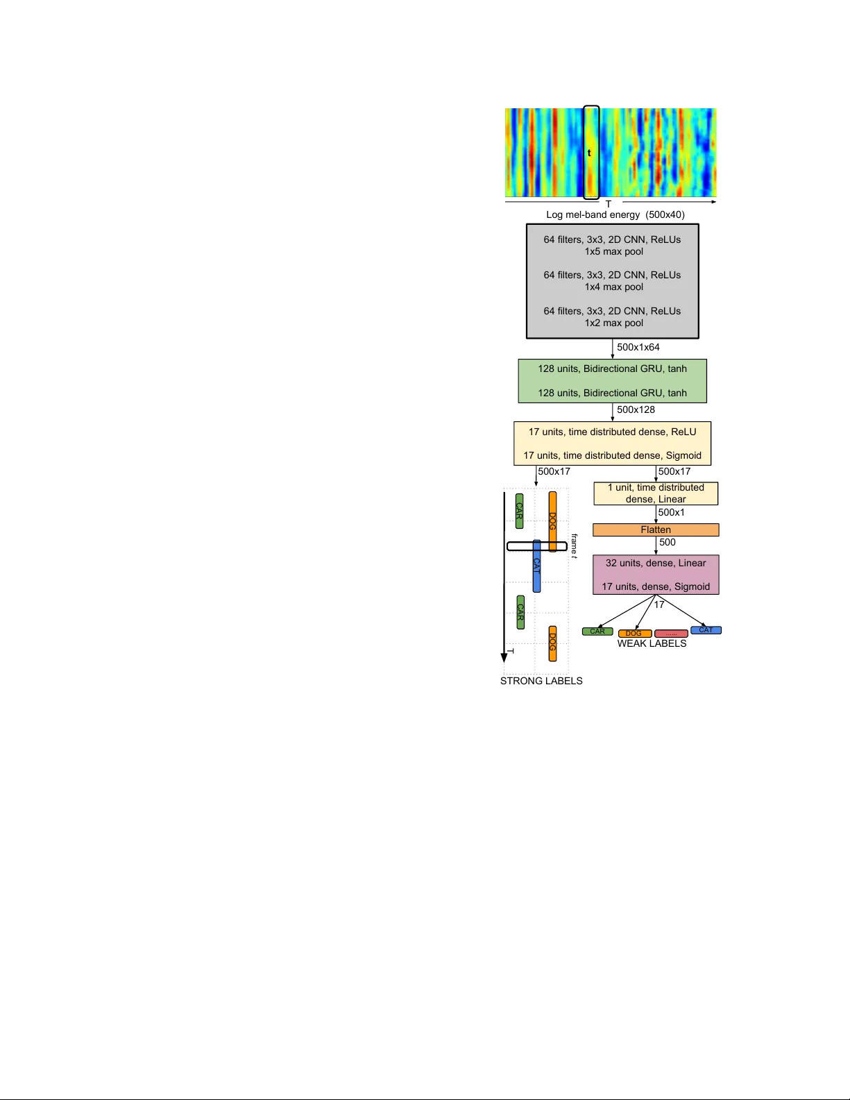
Detection and Classification of Acoustic Scenes and Events 2017 16 November 2017, Munich, German y SOUND EVENT DETECTION USING WEAKL Y LABELED D A T ASET WITH ST A CKED CONV OLUTIONAL AND RECURRENT NEURAL NETW ORK Sharath Adavanne , T uomas V irtanen Department of Signal Processing , T ampere Univ ersity of T echnology ABSTRA CT This paper proposes a neural network architecture and training scheme to learn the start and end time of sound events (strong la- bels) in an audio recording giv en just the list of sound e vents exist- ing in the audio without time information (weak labels). W e achie ve this by using a stacked conv olutional and recurrent neural network with two prediction layers in sequence one for the strong followed by the weak label. The netw ork is trained using frame-wise log mel- band energy as the input audio feature, and weak labels provided in the dataset as labels for the weak label prediction layer . Strong la- bels are generated by replicating the weak labels as many number of times as the frames in the input audio feature, and used for strong label layer during training. W e propose to control what the network learns from the weak and strong labels by different weighting for the loss computed in the tw o prediction layers. The proposed method is ev aluated on a publicly available dataset of 155 hours with 17 sound ev ent classes. The method achiev es the best error rate of 0.84 for strong labels and F-score of 43.3% for weak labels on the unseen test split. Index T erms — sound e vent detection, weak labels, deep neural network, CNN, GR U 1. INTR ODUCTION Sound e vent detection (SED) is the task of recognizing sound e vents and its respective start and end timings in an audio recording. Rec- ognizing such sound ev ents and its temporal information can be use- ful in different applications such as surveillance [1, 2], biodiv ersity monitoring [3, 4] and query based multimedia retrie val [5]. T ra- ditionally , SED has been tackled with datasets that have temporal information for each of the sound event present [6, 7]. W e refer to such temporal information of sound ev ents as strong labels in this paper . The internet has a vast collection of audio data. Many collab- orativ e and social websites like Freesound 1 and Y ouT ube 2 allow users to upload multimedia with metadata like captions a nd tags. W e can potentially automate the collection of audio data associated with a given tag from these online sources in considerably less time and manual effort. Recently , Gemekke et al. [8] carried out this with 632 sound event tags on Y ouTube and collected nearly two The research leading to these results has receiv ed funding from the Eu- ropean Research Council under the European Unions H2020 Framew ork Programme through ERC Grant Agreement 637422 EVER YSOUND. The authors also wish to acknowledge CSC-IT Center for Science, Finland, for computational resources. 1 https://freesound.org/ 2 https://www .youtube.com/ million 10 second audio recordings. While these tags indicate that the sound event is present in the audio recording, the tags do not contain the information as to ho w many times they occur or at what time the y occur . In this paper , we call such tags without an y tempo- ral information as weak labels. The task of identifying weak labels of an audio is also referred as audio tagging in literature [9, 10]. Collecting and annotating data with strong labels to train SED methods is a time-consuming task inv olving a lot of manual labor . On the other hand, collecting weakly labeled data takes much less time to annotate manually , since the annotator has to mark only the activ e sound event classes and not its exact time boundaries. If we can build SED methods which can learn strong labels from such weakly labeled data, then the methods can learn on a large amount of data. In this paper, we propose to implement such a strong label learning SED method using weakly labeled training data. Similar research of using weakly labeled data to learn strong labels has been done in neighboring audio domains such as mu- sic [11, 12], and bird classification [13, 14]. Liu et al. [11] used a fully con volutional neural network (FCN) to recognize instru- ments and tempo for each time frame of an audio clip giv en only the clip lev el information. The y further extended this network to sound event detection [15] and experimented on publicly av ailable datasets. The advantage of using an FCN is it can handle audio input of any length. On the other hand, the limitation is that the frame- wise strong labels are obtained by an upscaling layer which repli- cates segment-wise output to as many number of frames required. Similar FCN as [15] was proposed in [16] without the upscaling layer , thereby estimating labels for short segments of length 1.5 s instead of frame wise labels. The study compares the performance of this FCN with a V GG-like network [17] lik e network which out- puts sound event labels in segments of 1.5 s. The FCN network is trained using the entire audio, and its respecti ve weak label. On the other hand, the VGG network is trained on sub-segments of the en- tire audio, assuming that the recording lev el weak label annotation remains the same in all its sub-segments. The study showed that using an FCN performs better SED than using the VGG method. Kumar et al. [18] proposed a multiple instance learning (MIL) ap- proach [19] for this task, though the results were promising the ap- proach was claimed to be not scalable to large datasets by the same authors in [16]. Sound ev ents in real life most often overlap each other . A SED method which can recognize such overlapping sound events is re- ferred as polyphonic SED method. The state of the art for poly- phonic SED, trained using strong labels, was proposed recently in [20], where log mel-band energy feature was used along with a stacked con volutional and recurrent neural network and e valuated on multiple datasets. Similar stacked conv olutional and recurrent neural network has also been shown to outperform state of the art Detection and Classification of Acoustic Scenes and Events 2017 16 November 2017, Munich, German y methods in audio tagging tasks [9, 10]. Moti vated by the perfor- mance of this method in SED and audio tagging, in this paper, we propose to extend the method to perform both SED and audio tag- ging together , giv en only the audio and its respectiv e weak labels. In particular, we use the log mel-band audio feature extracted from the audio and extend the stacked con volutional and recurrent neural network to predict two outputs sequentially , the strong followed by the weak labels. T o train the proposed netw ork we generate dummy strong labels by replicating the weak labels as many times as the number of frames in the audio input feature. W e further propose to control the information that the network learns by separately scaling the loss calculated in the weak and strong prediction layers. Networks similar to the proposed stacked con volutional and neural network are the current state of the arts for audio tag- ging [9, 10]. This shows that the architecture is capable of learn- ing the relev ant information in temporal domain and mapping it to activ e classes. In this paper , we show that the proposed training scheme can extract this temporal information that the network is learning in the intermediate layers and can be used as strong labels. In comparison to previous works [15, 16], the proposed method sup- ports higher time resolution for strong labels by its inherent design. The feature extraction and the proposed network is described in Section 2. The dataset, metric and ev aluation procedure is discussed in Section 3. Finally , the results and discussions of the ev aluation performed are presented in Section 4. 2. METHOD Figure 1 shows the overall block diagram of the proposed method. The log mel-band energy feature e xtracted from the audio is fed to a stacked con volutional and recurrent neural network, which sequen- tially produces the strong labels followed by the weak labels. Audio features are calculated using overlapping windows on the input audio of length 10-seconds, resulting in T frames of the fea- ture. The proposed neural network maps these features into strong labels first, and further , the strong labels are mapped to weak labels. For an input of T frames, and a total number of sound classes C in the dataset, the network predicts C for each of the T time frames as strong label output and just C as weak label output. The predicted outputs for each of the sound class is in the continuous range of [0, 1], where one signifies the presence of the sound class and zero the absence. The details of the feature extraction and the network are presented below . 2.1. Featur e extraction Log mel-band energy ( mbe ) is extracted in 40 ms Hamming win- dows with 50% overlap. In total 40 mel bands are used in the 0- 22050 Hz range. For a giv en 10 second audio input, the feature extraction block produces a 500 × 40 output ( T = 500). 2.2. Neural netw ork The input to the proposed network is the T × 40 mbe feature as shown in Figure 1. The local shift-in variant features of this input are learned using CNN layers in the beginning. W e use a 3 × 3 receptiv e field and pad the output with zeros to k eep the size same as input in all our CNN layers. The max-pooling operation is performed along the frequency axis after every layer of CNN to reduce the dimension to T × 1 × N , where N is equal to the number of filters in the last CNN layer . W e do not perform max-pooling along the time axis to preserve the input time resolution. The CNN layers activ ation 64 filters, 3x3, 2D CNN, ReLUs 1x5 max pool 64 filters, 3x3, 2D CNN, ReLUs 1x4 max pool 64 filters, 3x3, 2D CNN, ReLUs 1x2 max pool 500x1x64 128 units, Bidirectional GRU, tanh 128 units, Bidirectional GRU, tanh 32 units, dense, Linear 17 units, dense, Sigmoid 17 units, time distributed dense, ReLU 17 units, time distributed dense, Sigmoid Flatten 1 unit, time distributed dense, Linear 500x128 500x17 500x1 500 17 DOG DOG CAT CAR CAR T frame t CAR DOG CAT …... WEAK LABELS STRONG LABELS Log mel-band energy (500x40) t T 500x17 Figure 1: Stacked conv olutional and recurrent neural network for learning strong labels from weak labels. is further fed to a bi-directional gated recurrent units (GRU) with tanh activ ation to learn the long-term temporal structure of sound ev ents, followed by time distributed fully-connected (dense) layers to reduce the feature-length dimensionality . The time resolution of T frames is unaltered in both the GR U and dense layers. Since we have to predict multiple labels simultaneously , we use sigmoid activ ation in the last dense layer . This prediction layer outputs the strong labels present in the input audio, and we refer to this as strong output in future. The dimensions of the strong labels are T × C . W e calculate the strong label loss on this output. Further, we reduce the activ ation dimensionality and remove the framing information using dense layers and map it to the C weak labels present in the audio. W e refer to this weak label prediction layer as weak output in future and calculate the weak label loss on its output. The total loss of the network is then calculated as the weighted sum of strong and weak losses. Detection and Classification of Acoustic Scenes and Events 2017 16 November 2017, Munich, German y During the training, the loss at weak and strong outputs was weighed dif ferently to facilitate learning from one output more than the other . In other words, during training, the weak labels along with the weighting scheme help control the learning of strong labels. On the other hand, during testing, the weak labels are obtained from the predicted strong labels. Batch normalization [21] is performed on the acti vations of ev- ery CNN layer . W e train the network for 1000 epochs using binary cross-entropy loss function for both the strong and weak outputs, and Adam [22] optimizer . Early stopping was used to reduce the ov erfitting of the network to training data. The training was stopped if the sum of the error rate of strong labels and F-score of weak la- bels (see Section 3.2) referred as the training metric in future did not improv e for more than 100 epochs. W e used dropout[23] after ev- ery layer of the network as a regularizer to mak e the training generic and work on unseen data. The implementation of the network was done using Keras [24] with Theano [25] as back end. 3. EV ALU A TION 3.1. Dataset The method is e valuated using a subset of the recently released Au- dioset data by Google [8]. This subset was organized as part of a challenge in the Detection and Classification of Acoustic Scenes and Events (DCASE) [26]. The dataset consists of a training, testing and evaluation split. The training split consists of 51,172 recordings, and the testing split consists of 488 recordings. All recordings are of 10-second length, monochannel and sampled at 44100 Hz. All these recordings hav e been collected from publicly uploaded Y outube videos as e xplained in [8]. Different methods trained on this training and testing split were benchmarked using the unseen ev aluation split of 1103 record- ings at the DCASE 2017 challenge [26]. The dataset contains 17 labels in total and each recording can hav e more than one label. Strong labels are provided only for the testing split, while weak labels are provided for both the splits. In order to train our network, we need strong labels in the training data as well. W e generate this by replicating the weak labels for every time frame of the audio and use them as strong labels. 3.2. Metric W e ev aluate our method in a similar fashion as the challenge [26]. Evaluation are performed indi vidually on the weak and strong label predictions. The weak labels are e valuated by calculating the total num- ber of recalls ( R ), its respective precision ( P ) and the F-score as R = T P / ( T P + F N ) , P = T P / ( T P + F P ) and F = 2 · P · R / ( P + R ) respectively . Where, true positiv es ( T P ) is the number of times the method correctly predicted the ground-truth label. False positiv es ( F P ) is the number of times the method pre- dicted incorrectly the ground-truth labels. False negativ e ( F N ) is the number of times the method did not predict a ground-truth label. The strong labels are evaluated using a segment based F-score and error rate (ER) as proposed in [27]. According to which the F-score is calculated as F = 2 · P K k =1 T P ( k ) 2 · P K k =1 T P ( k ) + P K k =1 F P ( k ) + P K k =1 F N ( k ) , (1) where T P ( k ) , F P ( k ) and F N ( k ) are the true positi ves, f alse pos- itiv es and false negati ves respectiv ely calculated for each of the K segments. The ER is calculated as E R = P K k =1 S ( k ) + P K k =1 D ( k ) + P K k =1 I ( k ) P K k =1 N ( k ) , (2) where N ( k ) is the total number of labels active in a given segment k . S ( k ) , D ( k ) and I ( k ) are the substitutions, deletions and inser- tions respectiv ely measured for each of the K segments as S ( k ) = min( F N ( k ) , F P ( k )) , D ( k ) = max(0 , F N ( k ) − F P ( k )) and I ( k ) = max(0 , F P ( k ) − F N ( k )) . W e use a segment length of one second for our strong label metrics. The ideal F-score is 100 and ER is zero. 3.3. Baseline The baseline method for the dataset is pro vided by [26]. It is a basic method to provide a comparison point for other methods using the dataset. This baseline method uses mbe as the audio feature. The network used is a fully-connected one with tw o hidden layers, each with 50 units and 20% dropout, follo wed by a prediction layer with as many sigmoid units as the number of classes in the dataset. A context of fiv e frames of the audio feature is used for training the network along with binary cross-entropy loss and Adam optimizer . The ev aluation metric scores for the baseline method are shown in T able 1. The network is trained by replicating the weak labels as many number of times as the number of frames in the input audio feature. During testing, the weak labels are obtained outside the network by identifying the sound e vents acti ve in the strong labels. 3.4. Evaluation procedur e The stacked conv olutional and recurrent neural network is trained with mbe as input, the weak labels provided in the dataset as weak output and the strong labels generated by replicating weak labels for each time frame as strong output. Giv en that the data is huge and the hardware has memory con- straints, the training time can be long (about 1800 s/epoch on our hardware). W e cannot perform an extensiv e hyperparameter search in the limited time, hence we start with a similar network configura- tion as in [7], and perform a random search [28] by varying the num- ber of units/filters in each of the layers until no under or ov er-fitting is observed while having a strong training metric. Since the dataset is large and is uploaded by different users, we assume that there will be enough variability and hence do not use any regularizer . The best configuration with highest training metric is as shown in Figure 1. This configuration has around 218,000 parameters. Other configu- rations with higher number of parameters, up to 2,000,000, did not show an y substantial improv ement over the chosen configuration. On finalizing the network, in order to be sure of our assump- tion that the high variability in data will not result in an over -fitting model, we experiment using dropout for each layer in our network as a regularizer and v ary it in the set of { 0.05, 0.15, 0.25, 0.5 and 0.75 } . W e use the same dropout for all layers in this study . The weights for the two prediction layers were experimented with different combinations in the logarithmic set of { 0.002, 0.02, 0.2, 1 } . The number 0.002 is motivated from the ratio of the to- tal number of time frames for the weak label (1) to the number of frames for the strong label (500). Detection and Classification of Acoustic Scenes and Events 2017 16 November 2017, Munich, German y W eak labels Strong labels Dropout P R F ER F Baseline [26] 12.2 14.1 13.1 1.02 13.8 0.05 44.6 37.8 40.9 0.86 38.6 0.15 47.5 39.7 43.3 0.84 38.8 0.25 43.0 35.0 38.6 0.86 33.8 0.5 21.5 17.3 19.2 0.99 8.6 0.75 12.3 9.9 11.0 1.15 8.0 T able 1: Evaluation metric scores for weak and strong labels for different dropout v alues. 4. RESUL TS AND DISCUSSION The e valuation metric scores for weak and strong labels for dif ferent dropout values tried are compared in T able 1. The best training metric of 43.3% F-score for weak labels and 0.84 ER for strong labels was achieved with 0.15 dropout for the proposed network. This study was performed by having the same weight of one for weak and strong outputs during training. In comparison with the baseline [26] score of 1.02 ER for strong labels and 13.1% F-score for weak labels, this is a significant improv ement. W e used the above-estimated dropout of 0.15 and studied how the network learns when provided with different weights for weak and strong outputs and present the results in T able 2. For example, from the first row of the table, the loss at strong output was scaled with 0.002 while the loss at weak output was unscaled. Since the strong labels for training were generated by replicating the weak labels, they are not the actual true labels, hence by intuition, we assumed higher weighting for weak labels will give better training metric. From experimentation, it was seen that the best training metric was actually obtained by using the same weight of one for both the weak and strong outputs. Another interesting observation is that the ER and F-score for strong labels improve when strong output is given more weight than the weak output, even though the strong labels used while training is ‘weak’ in the sense of correct- ness. On the other hand, this also results in poor metric for weak labels. W e analyzed the predicted labels of our configuration with an equal weight of one for weak and strong outputs which achie ved the best training metric. Among the weak labels, the vehicular sound ev ents - train and skateboard, warning e vents - fire engine siren and civil defense siren were seen to have the highest F-scores of over 60%. On the other hand, sound e vents - ambulance siren, car alarm, car passing, rev erse beeps, train horn had zero F-score. The same sound ev ents and the trend were observed for strong labels. In order to understand what our method is learning, we visual- ized the acti vations in the first con volutional layer of the network for a giv en output class. The visualizations are done using the saliency map [29] approach implementation in keras-vis [30]. The saliency map is the gradient of output class with respect to the input fea- ture. An example of such visualization is shown in Figure 2 for the recording ‘–jc0NAxK8M 30.000 40.000’ in the test dataset. The top and center sub-plots are the acti vations of the first con volutional layer for the strong and weak output of sound class ‘car’. The bot- tom subplot shows the ground truth marked in red dotted line over the input mbe feature. W e see from the acti vation map of both strong and weak heat maps that the network is actually learning the sound ev ent from a relev ant time period in the mbe feature. Strong W eight W eak W eight W eak labels Strong labels P R F F ch ER F ER ch F ch 0.002 1 44.9 37.0 40.5 1.38 10.9 0.02 1 44.2 36.5 40.0 1.13 17.0 0.2 1 47.5 39.6 43.2 46.6 0.84 38.1 0.80 48.3 1 1 47.5 39.7 43.3 45.5 0.84 38.8 0.81 47.9 1 0.2 47.3 39.5 43.0 44.5 0.84 38.6 0.82 48.9 1 0.02 25.5 20.6 22.8 0.81 41.1 1 0.002 20.5 16.5 18.3 26.3 0.81 42.4 0.79 49.0 T able 2: Evaluation metric scores for dif ferent combinations of weights for strong and weak label loss. The scores with subscript ch represents the challenge results. 0 100 200 300 400 500 40 20 0 40 20 0 40 20 0 Figure 2: V isualization of the activ ations in the first layer of CNN for strong (top) and weak (center) prediction of sound e vent class ‘car’ in ‘–jc0NAxK8M 30.000 40.000’ recording. The bottom plot shows the input to the network, the log mel-band feature of the recording, where the sound ev ent class is active in the region bounded by the red dotted line. 4.1. DCASE 2017 challenge results The results of the proposed method on the ev aluation split of DCASE 2017 challenge [26] is presented in T able 2. Four systems with dif ferent strong and weak output weighting were chosen based on their performance on test split. Similar trend of better strong label score when strong output is weighed more was observed on ev aluation data (ER ch = 0.79) as well. In comparison, [31] obtained the best weak label F-score of 55.6% and [32] obtained the best strong label error rate of 0.66. 5. CONCLUSION The task of learning temporal information of sound ev ents in an audio recording, giv en only the sound ev ents existing in the audio without the time information is tackled in this paper . A stacked con volutional and recurrent neural network architecture with two prediction layer outputs and a training scheme was proposed in this regard. This network was trained using different weights for the loss calculated in the two prediction layers. Even though the strong labels used for training were just repeated weak labels, it was ob- served that the network learned the relev ant strong labels correctly when the weighting for the two prediction layers was equal. This ev aluation was carried out on a publicly available dataset of 155 hours duration. An error rate of 0.84 for strong labels and F-score of 43.3% for weak labels was achie ved on the test data. Detection and Classification of Acoustic Scenes and Events 2017 16 November 2017, Munich, German y 6. REFERENCES [1] A. Harma, M. F . McKinney , and J. Skowronek, “ Automatic surveillance of the acoustic acti vity in our living en viron- ment, ” in IEEE International Conference on Multimedia and Expo (ICME) , 2005. [2] M. Crocco, M. Cristani, A. Trucco, and V . Murino, “ Audio surveillance: A systematic revie w , ” in ACM Computing Sur- ve ys (CSUR) , 2016. [3] K. J. Piczak, “En vironmental sound classification with con vo- lutional neural networks, ” in IEEE International W orkshop on Machine Learning for Signal Pr ocessing (MLSP) , 2015. [4] S. Chu, S. Narayanan, and C. J. Kuo, “En vironmental sound recognition with time-frequency audio features, ” in IEEE T ransactions on Audio, Speech, and Language Processing , 2009. [5] M. Xu, C. Xu, L. Duan, J. S. Jin, and S. Luo, “ Audio key- words generation for sports video analysis, ” in ACM T ransac- tions on Multimedia Computing , Communications, and Appli- cations (TOMM) , 2008. [6] “Sound e vent detection in real life audio. ” Detection and Classification of Acoustic Scenes and Events (DCASE), 2016. [Online]. A vailable: http://www .cs.tut.fi/sgn/arg/dcase2016/ task- sound- ev ent- detection- in- real- life- audio [7] S. Adav anne, P . Pertil ¨ a, and T . V irtanen, “Sound e vent de- tection using spatial features and con volutional recurrent neu- ral network, ” in IEEE International Conference on Acoustics, Speech and Signal Pr ocessing (ICASSP) , 2017. [8] J. F . Gemmeke, D. P . W . Ellis, D. Freedman, A. Jansen, W . Lawrence, R. C. Moore, M. Plakal, and M. Ritter , “ Audio set: an ontology and human-labeled dataset for audio events, ” in IEEE International Conference on Acoustics, Speech and Signal Pr ocessing (ICASSP) , 2017. [9] Y . Xu, Q. Kong, Q. Huang, W . W ang, and M. D. Plumbley , “Con volutional gated recurrent neural network incorporating spatial features for audio tagging, ” in International J oint Con- fer ence on Neural Networks (IJCNN) , 2017. [10] S. Adav anne, K. Drossos, E. Cakir , and T . V irtanen, “Stacked con volutional and recurrent neural networks for bird audio detection, ” in Eur opean Signal Processing Confer ence (EU- SIPCO) , 2017. [11] J.-Y . Liu and Y .-H. Y ang, “Event localization in music auto- tagging, ” in A CM on Multimedia Conference , 2016. [12] M. I. Mandel and D. P . W . Ellis, “Multiple-instance learning for music information retriev al, ” in International Confer ence of Music Information Retrieval (ISMIR) , 2008. [13] J. F . Ruiz-Munoz, M. Orozco-Alzate, and G. Castellanos- Dominguez, “Multiple instance learning-based birdsong clas- sification using unsupervised recording segmentation, ” in In- ternational Joint Confer ence on Artificial Intelligence , 2015. [14] F . Briggs, B. Lakshminarayanan, L. Neal, X. Z. Fern, R. Raich, S. J. K. Hadley , A. S. Hadley , and M. G. Betts, “ Acoustic classification of multiple simultaneous bird species: a multi-instance multi-label approach, ” in The Journal of the Acoustical Society of America , 2012. [15] T .-W . Su, J.-Y . Liu, and Y .-H. Y ang, “W eakly-supervised au- dio ev ent detection using event-specific gaussian filters and fully conv olutional networks, ” in IEEE International Confer- ence on Acoustics, Speech and Signal Processing (ICASSP) , 2017. [16] A. Kumar and B. Raj, “Deep CNN frame work for au- dio event recognition using weakly labeled web data, ” in arXiv:1707.02530v2 , 2017. [17] K. Simonyan and A. Zisserman, “V ery deep con volutional networks for large-scale image recognition, ” in International Confer ence on Learning Repr esentations (ICLR) , 2015. [18] A. Kumar and B. Raj, “ Audio event detection using weakly labeled data, ” in A CM on Multimedia Conference , 2016. [19] T . G. Dietterich, R. H. Lathrop, and T . Lozano-Prez, “Solving the multiple instance problem with axis-parallel rectangles, ” in International Joint Conference on Artificial Intelligence , 1997. [20] E. C ¸ akır , G. Parascandolo, T . Heittola, H. Huttunen, and T . V irtanen, “Con volutional recurrent neural networks for polyphonic sound event detection, ” in IEEE/ACM T ASLP , vol- ume 25, issue 6, 2017. [21] S. Ioffe and C. Szegedy , “Batch normalization: Accelerating deep network training by reducing internal covariate shift, ” CoRR , vol. abs/1502.03167, 2015. [22] D. Kingma and J. Ba, “ Adam: A method for stochastic opti- mization, ” in arXiv:1412.6980 [cs.LG] , 2014. [23] N. Sri vasta va, G. Hinton, A. Krizhe vsky , I. Sutske ver , and R. Salakhutdinov , “Dropout: A simple way to prevent neural networks from ov erfitting, ” in Journal of Machine Learning Resear ch (JMLR) , 2014. [24] F . Chollet, “Keras v1.1.2, ” https://github .com/fchollet/keras, 2015. [25] Theano De velopment T eam, “Theano: A Python frame- work for fast computation of mathematical expressions, ” in arXiv:1605.02688 , 2016. [26] A. Mesaros, T . Heittola, A. Diment, B. Elizalde, A. Shah, E. V incent, B. Raj, and T . V irtanen, “DCASE 2017 challenge setup: tasks, datasets and baseline system, ” in Detection and Classification of Acoustic Scenes and Events 2017 W orkshop (DCASE) , 2017, submitted. [27] A. Mesaros, T . Heittola, and T . V irtanen, “Metrics for poly- phonic sound event detection, ” in Applied Sciences , vol. 6(6):162, 2016. [28] J. Bergstra and Y . Bengio, “Random search for hyper- parameter optimization, ” in Journal of Machine Learning Re- sear ch , 2012. [29] K. Simonyan, A. V edaldi, and A. Zisserman, “Deep in- side conv olutional networks: V isualising image classification models and saliency maps, ” in , 2013. [30] R. K otikalapudi, “Keras V isualization T oolkit, ” 2017. [Online]. A v ailable: https://github.com/raghakot/k eras- vis [31] Y . Xu, Q. Kong, Q. Huang, W . W ang, and M. D. Plumbley , “T echnical report: Surrey-CVSSP system for DCASE2017 challenge task4, ” 2017. [32] K. Lee, D. Lee, S. Lee, and Y . Han, “T echnical report: Ensem- ble of conv olutional neural networks for weakly-supervised sound ev ent detection using multiple scale input, ” 2017.