An expressive dissimilarity measure for relational clustering using neighbourhood trees

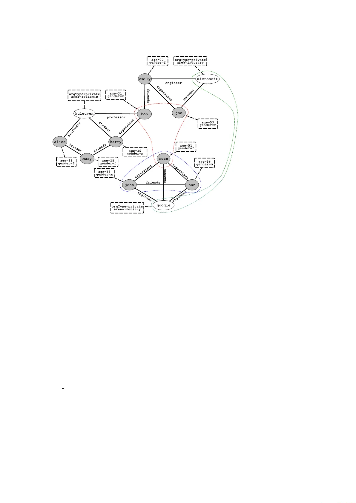
Noname manuscript No. (will be inserted by the editor) An expressiv e dissimilarity measure f or relational clustering using neighbourhood trees Sebastijan Duman ˇ ci ´ c · Hendrik Blockeel Receiv ed: date / Accepted: date Abstract Clustering is an underspecified task: there are no universal criteria for what makes a good clustering. This is especially true for relational data, where similarity can be based on the features of individuals, the relationships between them, or a mix of both. Existing methods for relational clustering ha ve strong and often impli cit biases in this respect. In this paper , we introduce a novel dissimilarity measure for relational data. It is the first approach to incorporate a wide variety of types of similarity , including similarity of attributes, similar- ity of relational context, and proximity in a hypergraph. W e experimentally ev aluate the pro- posed dissimilarity measure on both clustering and classification tasks using data set of very different types. Considering the quality of the obtained clustering, the e xperiments demon- strate that (a) using this dissimilarity in standard clustering methods consistently gi ves good results, whereas other measures work well only on data sets that match their bias; and (b) on most data sets, the novel dissimilarity outperforms even the best among the existing ones. On the classification tasks, the proposed method outperforms the competitors on the major- ity of data sets, often by a lar ge margin. Moreover , we show that learning the appropriate bias in an unsupervised way is a very challenging task, and that the e xisting methods offer a marginal gain compared to the proposed similarity method, and can e ven hurt performance. Finally , we show that the asymptotic complexity of the proposed dissimilarity measure is similar to the existing state-of-the-art approaches. The results confirm that the proposed dissimilarity measure is indeed versatile enough to capture relev ant information, regardless of whether that comes from the attributes of vertices, their proximity , or connectedness of vertices, e ven without parameter tuning. Keyw ords Relational learning · Clustering · Similarity of structured objects 1 Introduction In relational learning, the data set contains instances with relationships between them. Stan- dard learning methods typically assume data are i.i.d. (drawn independently from the same population) and ignore the information in these relationships. Relational learning methods Department of Computer Science, KU Leuven Celestijnenlaan 200A, Hev erlee, Belgium E-mail: { sebastijan.dumancic,hendrik.blockeel } @cs.kuleuven.be 2 Sebastijan Duman ˇ ci ´ c, Hendrik Blockeel do e xploit that information, and this often results in better performance. Complex data, such as relational data, is ubiquitous to the modern world. Among the most notable e xamples are social networks, which typically consist of a netw ork of people interacting with each other . Another example includes rich biological and chemical data that often contains man y interaction between atoms, molecules or proteins. Finally , any data stored in the form of relational databases is essentially relational data. Much research in relational learning fo- cuses on supervised learning (De Raedt, 2008) or probabilistic graphical models (Getoor and T askar, 2007). Clustering, howe ver , has receiv ed less attention in the relational conte xt. Clustering is an underspecified learning task: there is no univ ersal criterion for what makes a good clustering, it is inherently subjectiv e. This is kno wn for i.i.d. data (Estivill- Castro, 2002), and e ven more true for relational data. Dif ferent methods for relational clus- tering hav e very different biases, which are often left implicit; for instance, some methods represent the relational information as a graph (which means they assume a single binary relation) and assume that similarity refers to proximity in the graph, whereas other methods that take the relational database stance assume the similarity comes from relationships ob- jects participate in. Such strong implicit biases make use of a clustering algorithm difficult for a problem at hand, without a deep understanding of both the clustering method and the problem at hand. In this paper , we propose a very versatile framew ork for clustering relational data that makes the underlying biases transparent to a user . It views a relational data set as a graph with typed v ertices, typed edges, and attributes associated to the vertices. This view is very similar to the viewpoint of relational databases or predicate logic. The task we consider is clustering the vertices of one particular type. What distinguishes our approach from other approaches is that the concept of (dis)similarity used here is v ery broad. It can take into account attribute dissimilarity , dissimilarity of the relations an object participates in (in- cluding roles and multiplicity), dissimilarity of the neighbourhoods (in terms of attributes, relationships, or vertex identity), and interconnecti vity or graph proximity of the objects being compared. Consider for example Figure 1. This relational dataset describes people and organiza- tions, and relationships between them (friendship, a personss role in the organization, . . . ). Persons and organizations are vertices in the graph sho wn there (sho wn as white/gray el- lipses), the relationships between them are shown as edges, and their attributes are shown in dashed boxes. No w , vertices can be clustered in very dif ferent ways: 1. Google and Microsoft are similar because of their attrib utes, and could be clustered together for that reason 2. John , Rose and Han form a densely interconnected cluster 3. Bob , Joe and Rose share the property that the y fulfill the role of supervisor Non-relational clustering systems will yield clusters such as the first one; they only look at the attrib utes of individuals. Graph partitioning systems yield clusters of the second type. Some relational clustering systems yield clusters of the third type, which are defined by local structural properties. Most e xisting clustering systems hav e a very strong bias to wards “their” type of clusters; a graph partitioning system, for instance, cannot possibly come up with the { Google, Microsoft } cluster , since this is not a connected component in the graph. The new clustering approach we propose is able to find all types of clusters, and even clusters that can only be found by mixing the biases. The clustering approach and the corresponding dissimilarity measure that we propose are introduced in Section 2. Section 3 compares our approach to related work. Section 4 An expressi ve dissimilarity measure for relational clustering using neighbourhood trees 3 Fig. 1: An illustration of a relational data set containing people and organizations, and dif- ferent clusters one might find in it. Instances - people and organizations, are represented by vertices, while relationships among them are represented with edges. The rectangles list an associated set of attributes for the corresponding v ertex. ev aluates the approach, both from the point of view of clustering (the main goal of this work) as from the point of view of the dissimilarity measure introduced here (which can be useful also for , e.g., nearest neighbor classification). Section 5 presents conclusions. 2 Relational clustering over neighbourhood trees 2.1 Hypergraph Representation W ithin relational learning, at least three different paradigms exist: inducti ve logic program- ming (Muggleton and De Raedt, 1994), which uses first-order logic representations; rela- tional data mining (Dzeroski and Blockeel, 2004), which is set in the context of relational databases; and graph mining (Cook and Holder, 2006), where relational data are represented as graphs. W e illustrate the different types of representation in Figure 2. This example rep- resents a set of people and organizations, and relationships between them. The relational database format (b) is perhaps the most familiar to most people. It has a table for each entity type ( Person, Organization ) and for each relationship type between entities ( Works for, Friends ). Each table contains multiple attributes, each of which can be 4 Sebastijan Duman ˇ ci ´ c, Hendrik Blockeel Fig. 2: Representation paradigms of relational data. Section a) represents the relational data set as a set of logical facts; the upper part represents the definition of each predicate, while the bottom part lists all facts. Section b) illustrates a database view of the relational data set, where each logical predicate is associated with a single database table. Section c) illustrates a graph view of the relational data set. Each circle represents an instance, each rectangle rep- resents attributes associated with the corresponding instance, while relations are represented by the edges. an identifier for a particular entity (a key attribute , e.g., PName ), or a property of that en- tity ( Age,Gender,... ). The logic-based format (a) is very similar; it consists of logical facts, where the predicate name corresponds to the tables name and the arguments to the attribute values. There is a one-to-one mapping between rows in a table and logical facts. The logic based view allows for easy integration of background knowledge (in the form of first-order logic rules) with the data. Finally , there is the attributed graph representation (c) , where entities are nodes in the graph, binary relationships between them are edges, and nods and edges can have attributes. This representation has the advantage that it mak es the entities and their connecti vity more explicit, and it naturally separates identifiers from real attributes (e.g., the PName attribute from the Person table is not listed as an attribute of Person nodes, because it only serves to uniquely identify a person, and in the graph representation the node itself performs that function). A disadv antage is that edges in a graph can represent only binary relationships. Though the different representations are largely equiv alent, they provide dif ferent views on the data, which affects the clustering methods used. For instance, a notion such as shortest path distance is much more natural in the graph vie w than in the logic based vie w , while the An expressi ve dissimilarity measure for relational clustering using neighbourhood trees 5 fact that there are different types of entities is more explicit in the database view (one table per type). The distinction between entities and attrib ute values is explicit in the graph, but more implicit in the database view (key vs. non-key attributes) and absent in the logic view . In this paper , we will use a hypergraph view that combines elements of all the abov e. An oriented hypergraph is a structure H = ( V , E ) where V is a set of vertices and E a set of hyperedges; a hyperedge is an ordered multiset whose elements are in V . Directed graphs are a special case of oriented hypergraphs where all h yperedges hav e cardinality two. A set of relational data is represented by a typed, labeled, oriented hypergraph ( V , E , τ , λ ) with V a set of vertices, E a set of hyperedges, and τ : ( V ∪ E ) → T V ∪ T E a type function that assigns a type to each vertex and hyperedge ( T V is the set of vertex types, T E the set of hyperedge types). W ith each type t ∈ T V a set of attributes A ( t ) is associated, and λ maps each verte x v to a vector of values, one value for each attribute in A ( τ ( v )) . If a ∈ A ( τ ( v )) , we write a ( v ) for the v alue of a in v . A relational database can be con verted into the hypergraph representation as follows. 1 For each table with only one key attrib ute (describing the entities identified by that key), a vertex type is introduced, whose attrib utes are the non-key attributes of the table. Each row becomes one vertex, whose identifier is the key value and whose attribute values are the non-key attrib ute values in the ro w . For each table with more than one key attrib ute (de- scribing non-unary relationships among entities), a hyperedge is introduced that contains the vertices corresponding to these entities in the order they occur in the table. Our hypergraph representation does not associate attributes with hyperedges, only with vertices; hence, for non-unary relationships contain non-key attributes, a new verte x type corresponding to that hyperedge type is introduced. The clustering task we consider is the following: giv en a v ertex type t ∈ T V , partition the vertices of this type into clusters such that v ertices in the same cluster tend to be similar, and vertices in dif ferent clusters dissimilar, for some subjecti ve notion of similarity . In practice, it is of course not possible to use a subjecti ve notion; one uses a well-defined similarity function, which hopefully on average approximates well the subjectiv e notion that the user has in mind. The follo wing section introduces neighbourhood tr ees , a structure we use to compactly represent and describe a neighbourhood of a verte x. 2.2 Neighbourhood tree A neighbourhood tree is a directed graph rooted in a verte x of interest, i.e. the verte x whose neighbourhood one wants to describe. It is constructed simply by following the hyperedges from the root vertex, as outlined in Algorithm 1. The construction of the neighbourhood tree is parametrized with the pre-specified depth, a verte x of interest and the original hyper - graph. Consider a verte x v . For every hyperedge E in which v participates (lines 7-13), add a directed edge from v to each verte x v 0 ∈ E (line 9). Label each vertex with its type, and attach to it the corresponding attribute vector (line 10). Label the edge with the hyperedge type and the position of v in the hyperedge (recall that hyperedges are ordered sets; line 11). The vertices thus added are said to be at depth 1. If there are multiple hyperedges connecting vertices v and v 0 , v 0 is added each time it is encountered. Repeat this procedure for each v 0 on depth 1 (stored in v ariable toVisit ). The vertices thus added are at depth 2. Continue this procedure up to some predefined depth d . The root element is ne ver added to the subsequent lev els. An example of a neighbourhood tree is giv en in Figure 3. 1 For the logic-based representation, the con version is analogous. 6 Sebastijan Duman ˇ ci ´ c, Hendrik Blockeel Algorithm 1: Neighbourhood tree construction Data: a hypergraph H = ( V , E , τ , λ ) a vertex of interest v a depth d Result: a neighbourhood tree NT / * initialize neighbourhood tree * / 1 NT = new neighbourhood tree; 2 NT . addRoot (v); 3 NT . labelVertex (v) ; / * add type and attributes * / 4 toVisit = { v } ; / * vertices to process * / 5 d 0 = 1 ; / * depth indicator * / / * repeat until the pre-specified depth * / 6 while d 0 ≤ d do 7 for each v’ ∈ toVisit do 8 for each outgoing edge e of vertex v’ do 9 for each vertex v 00 in hyper edge e do 10 NT . addVertex ( v 00 ); 11 NT . addEdge ( v 0 , v 00 ); 12 NT . labelVertex ( v 00 ) ; / * add type and attributes * / 13 NT . labelEdge ( v 0 , v 00 ) ; / * add edge type and position * / 14 toVisit = toVisit ∪ { v 00 } ; 15 end 16 end 17 toVisit = toVisit \ { v’,v } 18 end 19 d 0 += 1; 20 end The follo wing section introduces a dissimilarity measure for vertices of the hyper graph. 2.3 Dissimilarity measure The main idea behind the proposed dissimilarity measure is to e xpress a wide range of sim- ilarity biases that can emerge in relational data, as discussed and ex emplified in Section 1. The proposed dissimilarity measure compares two vertices by comparing their neighbour- hood trees. It does this by comparing, for each level of the tree, the distribution of vertices, attribute values, and outgoing edge labels observed on that level. Earlier work in relational learning has shown that distrib utions are a good way of summarizing neighbourhoods (Per- lich and Prov ost, 2006). The method for comparing distributions distinguishes between discrete and continuous domains. For discrete domains (vertices, edge types, and discrete attrib utes), the distribution simply maps each value to its relati ve frequenc y in the observed multiset of values, and the χ 2 -measure for comparing distributions (Zhao et al, 2011) is used. That is, given two multisets A and B , their dissimilarity is defined as d ( A , B ) = ∑ x ∈ A ∪ B ( f A ( x ) − f B ( x )) 2 f A ( x ) + f B ( x ) (1) where f S ( x ) is the relativ e frequenc y of element x in multiset S (e.g., for A = { a , b , b , c } , f A ( a ) = 0 . 25 and f A ( b ) = 0 . 5). An expressi ve dissimilarity measure for relational clustering using neighbourhood trees 7 Fig. 3: An illustration of the neighbourhood tree. The domain contains two types of vertices - objects ( A and B ) and elements ( C, D and E ), and two fictitious relations: R and F . The vertices of type object have an associated set of attributes. Section a) contains the database view of the domain. Section b) contains the corresponding hypergraph view . Here, edges are represented with full lines, while hyperegdges are represented with dashed lines. Finally , section c) contains the corresponding neighbourhood tr ee for the vertex A . In the continuous case, we compare distrib utions by applying aggre gate functions to the multiset of values, and comparing these aggregates. Given a set A of aggregate functions, the dissimilarity is defined as d ( A , B ) = ∑ f ∈ A f ( A ) − f ( B ) r (2) with r a normalization constant ( r = max M f ( M ) − min M f ( M ) , with M ranging ov er all multisets for this attribute observed in the entire set of neighbourhood trees). In our imple- mentation, we use the mean and standard deviation as aggre gate functions. The abov e methods for comparing distributions ha ve been chosen for their simplicity and ease of implementation. More sophisticated methods could be used. The main point of this section, howe ver , is which distributions are compared, not how the y are compared. W e use the following notation. F or any neighbourhood tree g , • V l ( g ) is the multiset of v ertices at depth l (the root having depth 0) • V l t ( g ) is the multiset of v ertices of type t at depth l 8 Sebastijan Duman ˇ ci ´ c, Hendrik Blockeel • B l t , a ( g ) is the multiset of values of attrib ute a observed among the nodes of type t at depth l • E l ( g ) is the multiset of edge types between depth l and l + 1 E.g., for the neighbourhood tree in Figure 3, we hav e • V 1 ( g ) = { B, C, D } • V 1 ob ject ( g ) = { B } • E 1 ( g ) = { ( F,1 ), ( R,1 ), ( R,1 ) } • B 1 ob ject , A t t r 1 ( g ) = { Y } Let N be the set of all neighbourhood trees corresponding to the vertices of interest in a hypergraph. Let norm ( · ) be a normalization oper ator , defined as norm ( f ( g 1 , g 2 )) = f ( g 1 , g 2 ) max g , g 0 ∈ N f ( g , g 0 ) , i.e., the normalization operator divides the value of the function f ( g 1 , g 2 ) of two neighbour - hood trees g 1 and g 2 by the highest value of the function f obtained amongst all pairs of neighbourhood trees. Intuitiv ely , the proposed method starts by comparing two v ertices according to their attributes. It then proceeds by comparing the properties of their neighbourhoods: which vertices are in there, which attributes they hav e and how are they interacting. Finally , it looks at the proximity of vertices in a gi ven hypergraph. Formally , the dissimilarity of two vertices v and v 0 is defined as the dissimilarity of their neighbourhood trees g and g 0 , which is: s ( g , g ) = w 1 · ad ( g , g ) + w 2 · nad ( g , g ) + w 3 · cd ( g , g ) + w 4 · nd ( g , g ) + w 5 · ed ( g , g ) (3) where ∑ i w i = 1 and – attribute-wise dissimilarity ad ( g , g 0 ) = nor m ∑ a ∈ A ( τ ( v )) d ( B 0 t , a ( g ) , B 0 t , a ( g 0 )) ! (4) measures the dissimilarity of the root elements v and v 0 according to their attribute-v alue pairs. – neighbourhood attribute dissimilarity nad ( g , g 0 ) = nor m d ∑ l = 1 ∑ t ∈ T V ∑ a ∈ A ( t ) d ( B l t , a ( g ) , B l t , a ( g 0 )) ! (5) measures the dissimilarity of attribute-v alue pairs associated with the neighbouring ver- tices of the root elements, per lev el and vertex type. – connection dissimilarity cd ( g , g 0 ) = 1 − nor m  |{ v ∈ V 0 ( g ) | v ∈ V 1 ( g 0 ) }|  (6) reflects the number of edges of different type that e xist between the two root elements. An expressi ve dissimilarity measure for relational clustering using neighbourhood trees 9 – neighbourhood dissimilarity nd ( g , g 0 ) = nor m # l evel s ∑ l = 1 ∑ t ∈ T v d ( V l t ( g ) , V l t ( g 0 )) ! (7) measures the dissimilarity of two root elements according to the vertex identities in their neighbourhoods, per lev el and vertex type. – edge distribution dissimilarity : ed ( g , g ) = nor m # l evel s ∑ l = 1 d ( E l ( g ) , E l ( g )) ! (8) measures the dissimilarity ov er edge types present in the neighbourhood trees, per le vel. Each component is normalized to the scale of 0-1 by the highest value obtained amongst all pair of vertices, ensuring that the influence of each factor is proportional to its weight. The weights w 1 − 5 in Equation 3 allow one to formulate a bias through the similarity measure. For the remainder of the text, we will term our approach as ReCeNT (for Relational Clustering using Neighbourhood Trees). The benefits and downsides of this formulation are discussed and contrasted to the existing approaches in Sections 3.3 and 4.3. This formulation is somewhat similar to the multi-view clustering (Bick el and Scheffer, 2004), with each of the components forming a different vie w on data. Ho wever , there is one important fundamental difference: multi-view clustering methods want to find clusters that are good in each view separately , whereas our components do not represent different views on the data, but different potential biases, which jointly contribute to the similarity measure. 3 Related work 3.1 Hypergraph representation T wo interpretations of the hypergraph view of relational data exist in literature. The one we incorporate here, where domain objects form vertices in a hypergraph with associated attributes, and their relationships form hyperedges, was first introduced by Richards and Mooney (1992). An alternati ve view , where logical facts form v ertices, is presented by Ong et al (2005). Such representations were later utilized to learn the formulas of relational mod- els by r elational path-finding (K ok and Domingos, 2010; Richards and Mooney, 1992; Ong et al, 2005; Lov ´ asz, 1996). The neighbourhood tree introduced in Section 2.2 can be seen as summary of all paths in a hypergraph originating at a certain vertex. Though neighbourhood trees and relational path-finding rely on a hyper graph view , the tasks they solve are conceptually different. Whereas the goal of the neighbourhood tree is to compactly represent a neighbourhood of a v ertex by summarizing all the paths originating at the verte x, the goal of relational path-finding is to identify a small set of important paths that appear often in a hypergraph. Additionally , a practical difference is the distinction between hyperedges and attributes - a neighbourhood tree is constructed by following only the hyperedges, while the mentioned work either treats attributes as unary hyperedges or requires a declarative bias from the user . 10 Sebastijan Duman ˇ ci ´ c, Hendrik Blockeel 3.2 Related tasks T wo problems related to the one we consider here are graph and tree partitioning (Bader et al, 2013). Graph partitioning focuses on partitioning the original graph into a set of smaller graphs such that certain properties are satisfied. Though such partitions can be seen as clus- ters of vertices, the clusters are limited to vertices that are connected to each other . Thus, the problem we consider here is strictly more general, and does not put any restriction of that kind on the cluster memberships; the (dis)similarity of vertices can originate in any of the (dis)similarity sources we consider , most of which cannot be expressed within a graph partitioning problem. A number of tree comparison techniques (Bille,2005) exists in the literature. These ap- proaches consider only the identity of vertices as a source of similarity , while ignoring the attributes and types of both vertices and hyperedges. Thus, they are not well suited for the comparison of neighbourhood trees. 3.3 Relational clustering The relational learning community , as well as the graph kernel community have previously shown interest in clustering relational (or structured) data. Existing similarity measures within the relational learning community can be coarsely divided into tw o groups. The first group consists of similarity measures defined ov er an attributed graph model (Pfeiffer et al, 2014), with e xamples in Hybrid similarity (HS) (Ne ville et al, 2003) and Hybrid similarity on Annotated Graphs (HSA G) (W itsenburg and Blockeel, 2011). Both ap- proaches focus on attrib ute-based similarity of vertices where HS compares the attrib utes of all connected v ertices, and HSA G’ s similariy measure compares attrib utes of the vertices themselves and attributes of their neighbouring vertices. The main limitations of these ap- proaches are that they ignore the existence of vertex and edge types, and impose a v ery strict bias to wards attributes of vertices. In comparison to the presented approach, HS defines dis- similarity as the ad component if there is an edge between two vertices, and ∞ otherwise. HSA G defines the dissimilarity as a linear combination of the ad and nad components for each pair of vertices. In contrast to the first group which employs a graph view , the second group of methods employs a predicate logic view , The two most prominent approaches are Conceptual clus- tering of Multi-r elational Data (CC) (Fonseca et al, 2012) and Relational instance-based learning (RIBL) (Emde and W ettschereck, 1996; Kirsten and Wrobel, 1998). CC firstly de- scribes each example (corresponding to a verte x in our problem) with a set of logical clauses that can be generated by a bottom clause saturation (Camacho et al, 2007). The obtained clauses are considered as features, and their similarity is measured by the T animoto similar - ity - a measure of overlap between sets. In that sense, it is similar to using the ad and ed components for generating clauses. Note that this approach does not differentiate between relations (or interactions) and attrib utes, does not consider distrib utions of any kind, and does not hav e a sense of depth of a neighbourhood. Finally , RIBL follows an intuition that the similarity of tw o objects depends on the similarity of their attributes’ values and the similarity of the objects related to them. T o that extent, it first constructs a context descrip- tor - a set of objects related to the object of interest, similarly to the neighbourhood trees. Comparing two object now inv olves comparing their features and computing the similarity of the set of objects they are linked to. That requires matching each object of one set to the An expressi ve dissimilarity measure for relational clustering using neighbourhood trees 11 T able 1: Aspects of similarity considered by different approaches. X denotes full consider- ation, w partial and × no consideration at all. Similarity Attributes Neighbourhood attributes Neighbourhood identities Proximity Structural properties ReCeNT X X X X X HS X × × × × HSA G X X × × × RIBL X X X × × CC w w × × w RKOH × w × × X WLST × w × × X most similar object in the other set, which is an e xpensiv e operation (proportional to the product of the set sizes). In contrast, the χ 2 distance is linear in the size of the multiset. Fur - ther , the χ 2 distance takes the multiplicity of elements into account (it essentially compares distributions), which the RIBL approach does not. W ithin the graph kernel community , two prominent groups exist: W eisfeiler -Lehman graph k ernels (WL) (Shervashidze et al, 2011; Shervashidze and Borgwardt, 2009; Frasconi et al, 2014; Haussler, 1999; Bai et al, 2014) and r andom walk based kernels (W achman and Khardon, 2007; Lov ´ asz, 1996). A common feature of these approaches is that they measure a similarity of graph by comparing their structural properties. The W eisfeiler-Lehman Graph Kernels is a family of graph kernels dev eloped upon the W eisfeiler-Lehman isomorphism test . The ke y idea of the WL isomorphism test is to extend the set of vertex attributes by the attributes of the set of neighbouring vertices, and compress the augmented attribute set into ne w set of attrib utes. There each ne w attribute of a vertex corresponds to a subtree rooted from the vertex, similarly to the neighbourhood trees. Sherv ashidze and Borgwardt hav e introduced a fast WL subtree kernel (WLST) (Sherv ashidze and Borgwardt, 2009) for undirected graphs by performing the WL isomorphism test to update the vertex labels, followed by counting the number of matched vertex labels. The dif ference between our approach and WL kernel family is subtle b ut important: WL graph kernels extend the set of attributes by identifying isomorphic subtrees present in (sub)graphs. This is reflected in the bias they impose, that is, the similarity comes from the structure of a graph (in our case, a neighbourhood tree). A Rooted Kernel for Order ed Hypergr aph (RK OH) (W achman and Khardon, 2007]) is an instance of random walk kernels successfully applied in relational learning tasks. These approaches estimate the similarity of two (hyper)graphs by comparing the walks one can obtain by trav ersing the hypergraph. RK OH defines a similarity measure that compares two hypergraphs by comparing the paths originating at every edge of both hypergraphs, instead of the paths originating at the root of the hyper graph. RKOH does not dif ferentiate between attributes and h yperedges, but treats e verything as an hyperedge instead (an attrib ute can be seen as an unary edge). T able 1 summarizes different aspects of similarity considered by the abov e mentioned approaches. The interpretations of similarity are divided into five sources of similarity . The first two categories concern attributes: attributes of the vertices themselves and their neigh- bouring vertices. The following two categories concern identities of vertices in the neigh- bourhood of a vertex of interest. They concern subgraphs (identity of vertices in the neigh- bourhood) centered at a vertex, and proximity of two vertices. The final category concerns 12 Sebastijan Duman ˇ ci ´ c, Hendrik Blockeel T able 2: Complexities of dif ferent approaches Appr oach Complexity HS O ( LA ) HSA G O  N 2 E A  ReCeNT O  N 2 E d  WLST O  N 2 E d  CC O  N 2  E + A l   RIBL O  N 2 ∏ d k = 1 ( E + A ) 2 k  RKOH O  N 2 ( E + A ) 2 d + 2 l  the structural properties of subgraphs in the neighbourhood of a verte x defined by the neigh- bourhood tree. 3.3.1 Complexity analysis Though scalability is not the focus of this work, here we show that the proposed approach is as scalable as the state-of-the-art kernel approaches, and substantially less complex than the majority of the abov e-mentioned approaches that use both attribute and link structure. For the sake of clarity of comparison, assume a homogeneous graph with only one vertex type and one edge type. Let N be the number of vertices in a hyper-graph, L be the total number of hyperedges, and d be the depth of a neighbourhood representation structure, where applicable. Let, as well, A be the number of attrib utes in a data set. Additionally , assume that all vertices participate in the same number of hyperedges, which we will refer to as E . W e will refer to the length of clause in CC and path in RKOH as l . T o compare any two vertices, ReCeNT requires one to compute the dissimilarity of the multisets representing the vertices, proportional to O ( d × A + ∑ d k = 1 E k ) = O  N 2 E d  . T able 2 summarizes the complexities of the discussed approaches. In summary , the approaches can be grouped into three categories. The first category contains HS and HSA G; these are substantially less complex than the rest, b ut focus only on the attribute similarities. The sec- ond cate gory contains RIBL and RKOH, which are substantially more complex than the rest. Both of these approaches use both attrib ute and edge information, b ut in a computa- tionally very expensiv e way . The last category contains ReCeNT , WLST and CC; these lie in between. They utilize both attribute and edge information, but in a w ay that is much more efficient than RIBL and RK OH. The comple xity of ReCeNT benefits mostly from two design choices: dif ferentiation of attributes and hyperedges , and decomposition of neighbourhood elements into multisets . By distinguishing hyperedges from attributes, ReCeNT focuses on identifying sparse neigh- bourhoods. Decomposition of neighbourhoods into multisets allo ws ReCeNT to compute the similarity linearly in the size of a multiset. The parameter that ReCeNT is the most sensitiv e to is the depth of the neighbourhood tree, which is the case with the state-of-the- art kernel approaches as well. Howe ver , the main underlying assumption behind ReCeNT is that important information is contained in small local neighbourhoods, and ReCeNT is designed to utilize such information. An expressi ve dissimilarity measure for relational clustering using neighbourhood trees 13 T able 3: Characteristics of the data sets used in e xperiments. The characteristics include the total number of vertices, the number of vertices of interest, the total number of attributes, the number of attributes associated with vertices of interest, the number of hyperedges as well as the number of different h yperedge types. data set IMDB UW -CSE Muta W ebKB T error #vertices 298 734 6124 3880 1293 #target vertices 268 272 230 920 1293 #vertex types 3 4 2 2 1 #attributes 3 7 7 1207 106 #target attributes 3 3 4 763 106 #hyper edges 715 1834 30804 5779 3743 #hyper edge types 3 6 7 4 2 4 Evaluation 4.1 Data sets W e ev aluate our approach on fi ve data sets for relational clustering with different charac- teristics and domains. The chosen data sets are commonly used within the (statistical) re- lational learning community , and they expose different biases. The characterization of data sets, summarized in T able 3, include the total number of vertices in a hypergraph, the num- ber of vertices of interest, the total number of attributes, the number of attributes associated with vertices of interest, the number of hyperedges as well as the number of different hy- peredge types. The data sets range from having a small number of vertices, attrib utes and hyperedges (UW -CSE, IMDB), to a considerably large number of vertices, attrib utes or hy- peredges (Mutagenesis, W ebKB, T erroristAttack). All the chosen data sets are originally classification data sets, which allo ws us to ev aluate our approach with respect to how well it extracts the classes present in the data set. The IMDB 2 data set is a small snapshot of the Internet Movie Database. It describes a set of movies with people acting in or directing them. The goal is to dif ferentiate people into two groups: actors and directors . The UW -CSE 3 data set describes the interactions of employees at the Univ ersity of W ashington and their roles, publications and the courses they teach. The task is to identify two clusters of people: students and pr ofessors . The Mutagenesis 4 data set, as described is Section 1, describes chemical compounds and atoms they consist of. Both compounds and atoms are described with a set of attributes describing their chemical properties. The task is to identify two clusters of compounds: mutagenic and not muta genic . The W ebKB 5 data set consists of pages and links collected from the Cornell University’ s webpage. Both pages and links are associated with a set of words appearing on a page or in the anchor text of a link. The pages are classified into sev en groups according to their role, such as personal , departmental or pr oject page. The final data set, termed T errorists 6 [Sen et al,2008], describes terrorist attacks each assigned one of 6 labels indicating the type of the attack. Each attack is described by a total of 106 distinct features, and two relations 2 A vailable at http://alchemy .cs.washington.edu/data/imdb 3 A vailable at http://alchemy .cs.washington.edu/data/uw-cse/ 4 A vailable at http://www .cs.ox.ac.uk/activities/machlearn/mutagenesis.html 5 A vailable at http://alchemy .cs.washington.edu/data/webkb/ 6 A vailable at http://linqs.umiacs.umd.edu/projects//projects/lbc/ 14 Sebastijan Duman ˇ ci ´ c, Hendrik Blockeel indicating whether two attacks were performed by the same organization or at the same location. 4.2 Experiment setup In the remainder of this section, we evaluate our approach. W e focus on answering the following questions: (Q1) How well does ReCeNT perform on the r elational clustering tasks compar ed to existing similarity measur es? (Q2) How r elevant is each of the components? W e perform clustering using our similarity measure and setting the parameters as w i = 1 , w j , j 6 = i = 0. (Q3) T o which extent can the parameters of the pr oposed similarity measur e be learnt fr om data in an unsupervised manner? (Q4) How well does ReCeNT perform compar ed to e xisting similarity measur es in a super- vised setting? (Q5) How do the runtimes for ReCeNT compare to the competitor s? In each experiment, we have used the aforementioned (dis)similarity measures in con- junction with spectral [Ng et al, 2001] and hierarchical [W ard, 1963] clustering algorithms. W e have intentionally chosen two clustering approaches which assume different biases, to be able to see how each similarity measure is af fected by assumptions clustering algorithms make. W e hav e altered the depth on neighbourhood trees between 1 and 2 wherev er it was possible, and report both results. W e e valuate each approach using the follo wing v alidation method: we set the number of clusters to be equal to the true number of clusters in each data set, and e valuate the obtained clustering with regards to how well it matches the known clustering gi ven by the labels. Each obtained clustering is then evaluated using the adjusted Rand index (ARI) [Rand, 1971; Morey and Agresti, 1984]. The ARI measures the similarity between two clusterings, in this case between the obtained clustering and the provided labels. The ARI score ranges between -1 and 1, where a score closer to 1 corresponds to higher similarity between two clusterings, and hence better performance, while 0 is the chance level. For each data set, and each similarity measure, we report the ARI score they achieve. Additionally , we hav e set a timeout to 24 hours and do not report results for an approach that takes more time to compute. T o achie ve a f air time comparison, we implemented all similarity measures (HS, HSA G, RIBL, CC, as well as RKOH) in Scala and optimized them in the same way , by caching all the intermediate results that can be re-used. W e have used the clustering algorithms im- plemented in Python’ s scikit-learn package [Pedregosa et al, 2011]. The hierarchy obtained by hierarchical clustering was cut when it has reached the pre-specified number of clusters. In the first experiment, the weights w 1 − 5 were not tuned, and were set to 0.2. W e hav e used mean and standard deviation as aggregates for continuous attrib utes. 4.3 Results 4.3.1 (Q1) Comparison to the existing methods W e compare ReCeNT to a pure attribute based approach (termed Baseline), HS [Neville et al, 2003], HSA G [W itsenbur g and Blockeel, 2011], CC [Fonseca et al, 2012], RIBL An expressi ve dissimilarity measure for relational clustering using neighbourhood trees 15 T able 4: Performance of all approaches on three data sets. For each similarity measure, the ARI achie ved when the true number of clusters was used. The results are shown for both hierarchical and spectral clustering,while the depth of the approaches is indicated by the subscript. The last column counts the number of wins per algorithm, where ”win” means achieving the highest ARI on a data set. Similarity Muta UWCSE W ebKB T error IMDB W H S H S H S H S H S Baseline -0.02 -0.03 0.25 0.2 0.00 0.25 0.00 0.17 0.05 0.05 0 HS N/A N/A 0.01 0.06 0.0 0.10 0.01 -0.01 0.00 0.00 0 CC 2 0.00 0.01 0.1 0.82 0.00 0.04 0.01 0.01 0.1 0.1 0 CC 4 0.00 0.01 0.00 0.92 0.00 0.04 0.01 0.01 0.1 0.1 0 ReCeNT 1 0.32 0.35 0.97 0.98 0.04 0.57 0.00 0.26 0.62 1.0 8 RIBL 1 0.22 0.26 0.89 0.68 0.0 0.1 N/A N/A 0.35 0.38 0 HSA G 1 -0.01 0.06 0.1 0.0 0.01 0.05 0.00 0.24 0.04 -0.05 0 WLST 1 , 5 0.00 0.02 -0.01 0.33 0.00 0.33 0.27 0.07 -0.01 0.66 1 WLST 1 , 10 0.00 0.02 -0.01 0.33 0.00 0.32 0.27 0.11 -0.01 0.31 1 V 1 0.00 0.03 -0.01 0.19 0.00 0.00 0.00 0.00 0.00 0.00 0 VE 1 0.00 0.03 0.01 0.36 0.00 0.00 0.00 0.00 1.0 1.0 2 RKOH 1 , 2 0.1 0.1 0.2 0.2 N/A N/A N/A N/A 0.83 0.83 0 RKOH 1 , 4 N/A N/A N/A N/A N/A N/A N/A N/A N/A N/A 0 ReCeNT 2 0.08 0.3 0.1 0.16 0.02 0.4 0.01 0.16 0.13 1.0 1 RIBL 2 N/A N/A 0.0 0.68 N/A N/A N/A N/A 0.63 0.78 0 HSA G 2 -0.01 0.06 0.1 0.0 0.0 0.04 0.00 0.23 0.04 0.09 0 WLST 2 , 5 0.00 0.01 0.02 0.02 0.00 0.52 0.27 0.11 -0.04 0.31 1 WLST 2 , 10 0.00 0.01 0.02 0.02 0.00 0.52 0.05 0.12 -0.04 0.36 0 V 2 0.00 0.07 0.01 0.00 0.00 0.00 0.00 0.00 0.00 0.00 0 VE 2 0.00 0.00 0.01 0.38 0.00 0.56 0.00 0.00 0.00 0.53 1 RKOH 2 , 2 N/A N/A N/A N/A N/A N/A N/A N/A N/A N/A 0 RKOH 2 , 4 N/A N/A N/A N/A N/A N/A N/A N/A N/A N/A 0 [Emde and W ettschereck, 1996], as well as W eisfeiler-Lehman subtree kernel (WLST) [Shervashidze and Borgwardt, 2009], Linear kernel between vertex histograms (V), Linear kernel between vertex-edge histograms (VE) provided with [Sugiyama and Borgw ardt,2015], and RKOH [W achman and Khardon, 2007]. The subscript in ReCeNT , HSA G, RIBL and kernel approaches denotes the depth of the neighbourhood tree (or other supporting struc- ture). The subscript in CC denotes the length of the clauses. The second subscript in WLST and RK OH indicates their parameters: with WLST it is the h parameter indicating the num- ber of iterations, whereas with RK OH it indicates the length of the walk. The results of the first experiment are summarized in T able 4. The table contains ARI values obtained by the similarity measures for each data set and clustering algorithm used. The last column of the table states the number of wins per approach. The number of wins is calculated by simply counting the number of cases where the approach obtained the highest ARI v alue, a ”case” being a combination of a data set and a clustering algorithm. ReCeNT 1 wins 8 out of 10 times, and thus outperforms all other methods. The best results are achiev ed in combination with spectral clustering, with exception being the T erroristAttack data set where WLST 1 , ∗ and WLST 2 , 5 combined with hierarchical clustering achieved the highest ARI of 0.27, in contrast to 0.26 obtained by ReCeNT 1 . In all cases of the Mutagenesis and UWCSE data sets, ReCeNT 1 wins with a larger margin. Howe ver , it is important to note that in the remaining cases, the closest competitor is not always the same. In the case of IMDB 16 Sebastijan Duman ˇ ci ´ c, Hendrik Blockeel data set in combination with spectral clustering, the closest competitor is VE 1 (together with RK OH 1 , 2 ), as well as in the case of W ebKB in combination with spectral clustering. In the cases of the T erroristAttack data set combined with the spectral clustering, the closest com- petitors are HSAG 1 and HSA G 2 , while in the case with hierarchical clustering our approach is outperformed by WLST 1 , ∗ and WLST 2 , 5 . These results show that the proposed similar- ity measure performs better over wide range of different tasks and biases, compared to the remaining approaches. Moreov er, when combined with the spectral clustering, ReCeNT 1 consistently performs well on all data sets, achieving the second-best result only on the T erroristAttack data set. Each of the data sets exposes different bias, which influences the performance of the methods. In order to successfully identify mutagenic compounds, one has to consider both attribute and link information, including the attributes of the neighbours. Chemical com- pounds that ha ve similar structure tend to have similar properties. This data set is more suitable for RIBL, ReCeNT and kernel approaches. ReCeNT 1 and RIBL 1 achiev e the best results here 7 , while kernels approaches surprisingly do not perform better than the chance lev el. The UW -CSE is a social-network-like data set where the task is to find two interact- ing communities with dif ferent attribute-v alues - students and professors. The distinction between tw o classes is made on a single attribute - professors have positions, while stu- dents do not, and the relation stating that professors advide students. This task is suitable for HS and HSA G. Ho wever , both approaches are substantially outperformed by ReCeNT 1 and CC ∗ . Similarly , the IMDB data set consists of a network of people and their roles in mo vies, which can be seen as a social network. Here, directors can be differentiated from actors by a single edge type - actors work under directors which is explicitly encoded in the data set. The type of interactions between entities matters the most, as it is not an attribute-rich data set, and is thus more suitable for methods that account for structural measures. Accordingly , ReCeNT , RIBL, WLST 1 , ∗ and VE kernels achie ve the best results. The remaining data sets, W ebKB and T erroristAttack, are entirely different in nature from the aforementioned ones. These data set have a substantially lar ger number of at- tributes, but those are not suf ficient to identify relev ant clusters supported by labels, that is, interactions contain important information. Such bias is implicitly present in HS, and partially assumed by kernel approaches. The results show that ReCeNT 1 and WSL T 2 , ∗ and VE 2 kernels achiev e almost identical performance on the W ebKB data set, while the remain- ing approaches are outperformed e ven by the baseline approach. On the T erroristAttack data set, WLST 1 , ∗ kernel achieves the best performance, outperforming ReCeNT 1 and HSAG 1 . Similarly to W ebKB, other approaches are outperformed by the baseline approach. The results summarized in T able 4 point to several conclusions. Firstly , giv en that the proposed approach achiev es the best results in 8 out of 10 test cases, the results suggest that it is indeed v ersatile enough to capture rele vant information, regardless of whether that comes from the attributes of vertices, their proximity , or connectedness of vertices, ev en without parameter tuning. Moreov er , when combined with the spectral clustering, our approach con- sistently obtains good results on all data sets, while the competitor approaches achie ve good results if the problem fits their bias. Secondly , the results show that one has to consider not only the bias of the similarity measure, but the bias of the clustering algorithm as well, which is evident on most data sets where spectral clustering achie ves substantially better perfor- mance than hierarchical clustering. Finally , ReCeNT and most of the approaches tend to be sensitiv e to the depth parameter, which is evident in the drastic dif ference in performance 7 W e were not able to make HS work on this data set as it assumes edges between compound vertices which are non-existing in this data set An expressi ve dissimilarity measure for relational clustering using neighbourhood trees 17 T able 5: Performance of ReCeNT with different parameter settings. The upper part of the table presents results with the neighbourhood trees with depth of 1, whereas the bottom part contains the results with depth set to 2. The parameters in italic indicate the best performance achiev ed. Parameters Muta UWCSE W ebKB T error IMDB Hier . Spec Hier . Spec Hier . Spec Hier . Spec Hier . Spec 1,0,0,0,0 0.00 0.00 0.25 0.2 0.00 0.25 0.01 0.17 0.05 0.05 0,1,0,0,0 0.00 0.00 0.52 0.12 0.00 0.00 0.00 -0.01 0.0 0.00 0,0,1,0,0 0.00 0.00 0.05 0.1 0.00 0.1 0.00 0.00 0.14 0.13 0,0,0,1,0 0.30 0.30 0.02 -0.03 0.00 0.2 0.00 -0.01 0.17 0.17 0,0,0,0,1 0.24 0.25 0.17 0.07 0.00 0.02 -0.01 0.00 1.0 1.0 0.2,0.2,0.2,0.2,0.2 0.32 0.35 0.96 0.86 0.04 0.56 0.00 0.26 0.62 1.0 1,0,0,0,0 0.00 0.00 0.00 0.2 0.00 0.27 0.00 0.17 0.05 -0.05 0,1,0,0,0 0.00 0.00 0.03 0.16 0.00 0.00 0.00 -0.01 0.0 0.00 0,0,1,0,0 0.00 0.00 0.00 0.08 0.00 0.01 0.01 0.00 0.15 0.13 0,0,0,1,0 0.29 0.29 0.01 -0.03 0.02 0.2 -0.01 -0.01 0.00 0.00 0,0,0,0,1 0.00 0.27 0.03 -0.04 0.00 0.02 0.00 0.00 1.0 1.0 0.2,0.2,0.2,0.2,0.2 0.08 0.3 0.1 0.07 0.02 0.4 0.01 0.16 0.13 1.0 when dif ferent depths are used. This suggests that increasing depth of a neighbourhood tree consequently introduces more noise. Interestingly , while the results suggest that with Re- CeNT the depth of 1 performs the best, the performance of kernel methods tend to increase with the depth parameter . These results justify the basic assumption of this approach that important information is contained in small local neighbourhoods. 4.3.2 (Q2) Relevance of components In the second experiment, we e v aluate how relev ant each of the fiv e components in Equa- tion 3 is. T able 5 summarizes the results. There are only two cases (Mutagenesis and IMDB) where using a single component (if it is the right one!) suffices to get results comparable to using all components (T able 5). This confirms that clustering relational data is difficult not only because one needs to choose the right source of similarity , but also because the similar- ity of relational objects may come from multiple sources, and one has to take all these into account in order to discov er interesting clusters. These results may explain why ReCeNT almost consistently outperforms all other meth- ods in the first experiment. First, ReCeNT considers different sources of relational similarity; and second, it ensures that each source has a comparable impact (by normalizing the impact of each source and giving each an equal weight in the linear combination). This guarantees that if a component contains useful information, it is taken into account. If a component has no useful information, it adds some noise to the similarity measure, but the clustering process seems quite resilient to this. If most of the components are irrelevant, the noise can dominate the pattern. This is likely what happens in experiment 1 when depth 2 neighbour- hood trees are used: too much irrelev ant information is introduced at level two, dominating the signal at lev el one. 18 Sebastijan Duman ˇ ci ´ c, Hendrik Blockeel T able 6: Results obtained by AASC. The subscript indicates the depth of the neighbourhood tree. Appr oach IMDB UWCSE Mutagenesis W ebKB T error ReCeNT 1 1.0 0.98 0.35 0.56 0.26 AASC 1 0.78 0.65 0.35 0.57 0.28 ReCeNT 2 1.0 0.07 0.3 0.4 0.16 AASC 2 0.67 0.23 0.3 0.4 0.23 4.3.3 (Q3) Learning weights in an unsupervised manner The first e xperiment sho ws that ReCeNT outperforms the competitor methods ev en without parameters being tuned. The second e xperiment sho ws that one typically has to consider multiple interpretations of similarity in order to obtain a useful clustering. A natural question to ask is whether the parameters could be learned from data in an unsupervised way . The possibility of tuning of fers an additional flexibility to the user . If the knowledge about the right bias is av ailable in advance, one can specify it through adjusting the parameters of the similarity measure, potentially achieving e ven better results than those presented in T able 4. Howe ver , tuning the weights in an automated and systematic way is a difficult task as there is no clear objecti ve function to optimize in a purely unsupervised settings. Many clustering ev aluation criteria, such as ARI, require a reference clustering which is not a vailable during clustering itself. Other clustering quality measures do not require a reference clustering, b ut each of those has its own bias (V an Craenendonck and Blockeel, 2015). An approach that might help in this direction is the Affinity Aggr egation for Spectral Clustering (AASC) (Huang et al, 2012). This work extends spectral clustering to a multi- ple affinity case. The authors start from the position that similarity of objects often can be measured in multiple ways, and it is often difficult to know in advance how different simi- larities should be combined in order to achieve the best results. Thus, the authors introduce an approach that learns the weights that would, when clustered into the desired number of clusters, yield the highest intra-cluster similarity . That is achie ved by iterati vely optimizing: (1) the cluster assignment given the fixed weights, and (2) weights given a fixed cluster as- signment. Thus, by treating each component in Equation 3 as a separate af finity matrix, this approach tries to learn their optimal combination. W e ha ve tried AASC in ReCeNT , and the results are summarized in T able 6. These results lead to sev eral conclusions. Firstly , in most cases AASC yields no substantial benefit or ev en hurts performance. This confirms that learning the appropriate bias (and the cor - responding parameters) in an entirely unsupervised way is a difficult problem. The main exceptions are found for depth 2: here, a substantial impro vement is found for UWCSE and T erroristAttack. This seems to indicate that the bad performance on depth 2 is indeed due to an o verload of irrelev ant information, and that AASC is able to weed out some of that. Still, the obtained results for depth 2 are not comparable to the ones obtained for depth 1. W e conclude that tuning the weights in an unsupervised manner will require more sophisticated methods than the current state of the art. 4.3.4 (Q4) P erformance in a supervised setting The previous experiments point out that the proposed dissimilarity measure performs well compared to the existing approaches, but finding the appropriate weights is dif ficult. Though An expressi ve dissimilarity measure for relational clustering using neighbourhood trees 19 T able 7: Performance of the kNN classifier with different (dis)similarity measure and weight learning. The performance is expressed in terms of accuracy ov er the 10-fold cross valida- tion. Appr oach IMDB UWCSE Mutagenesis W ebKB T errorists HS 88.08 76.66 0.00 12.78 27.51 CC 88.08 99.85 60.08 61.07 38.28 HSA G 88.08 95.88 77.40 12.82 75.62 ReCeNT 100 100 85.54 100 85.60 RIBL 100 77.22 76.37 84.11 N/A WLST 93.60 44.94 76.37 47.35 45.56 VE 100 98.26 70.60 49.33 30.00 V 93.80 43.61 70.42 47.35 44.39 RKOH 95.07 67.26 60.78 N/A N/A our focus is on clustering tasks, we can use our dissimilarity measure for classification tasks as well. The availability of labels offers a clear objecti ve to optimize when learning the weights, and thus allows us to e valuate the appropriateness of ReCeNT for classification. W e hav e set up an experiment where we use a k nearest neighbours (kNN) classifier with each of the (dis)similarity measures. It consists of a 10-fold cross-validation, where within each training fold, an internal 10-fold cross-validation is used to tune the parameters of the similarity measure, and kNN with the tuned similarity measure is next used to classify the examples in the corresponding test fold. The results of this experiment are summarized in T able 7. ReCeNT achie ves the best performance on all data sets. On the IMDB data set, ReCeNT achiev es perfect performance, as do RIBL and VE. On UWCSE, ReCeNT is 100% accurate; its closest competitor, CC, achiev es 99.85%. From the classification viewpoint, these two data sets are easy: the classes are differentiable by one particular attribute or relation. On Mutagenesis and T errorists, the difference is more outspoken: ReCeNT achiev es around 85% accuracy , with its clos- est competitor (HSAG) achieving 76% or 77%. On W ebKB, finally , ReCeNT and RIBL substantially outperform all the other approaches, with ReCeNT achie ving 100% and RIBL 84.11%. The remarkable performance of ReCeNT on W ebKB is e xplained by inspecting the tuned weights. These reveal that ReCeNT’ s ability to jointly consider verte x identity , edge type distrib ution, and v ertex attrib utes (in this case, words on webpages) are the reason why it performs so well. None of the other approaches take all three components into account, which is why they achie ve substantially worse results. These results clearly show that accounting for several views of similarity is beneficial for relational learning. Moreover , the av ailability of labelled information is clearly helpful and ReCeNT is capable of successfully adapting its bias tow ards the needs of the data set. 4.3.5 (Q5) Runtime comparison T able 8 presents a comparison of runtimes for each approach. All the experiments were run on a computer with 3.20 GHz of CPU power and 32 GB RAM. The runtimes include the construction of supporting structures (neighbourhood trees and context descriptors), calcu- lation of similarity between all pairs of vertices, and clustering. The measured runtimes are consistent with the previously discussed complexities of the approaches. HS, HSA G, CC, 20 Sebastijan Duman ˇ ci ´ c, Hendrik Blockeel T able 8: Runtime comparison in minutes (rounded up to the closest integer). The runtimes include the construction of supporting structures and time needed to calculate a similar- ity between each pair of vertices in a gi ven hypergraph. Note that graph kernel measures (in italic) are obtained using the external software provided with Sugiyama and Borgwardt (2015). N/A indicates that the calculation took more than 24 hours. Appr oach IMDB UWCSE Mutagenesis W ebKB T error HS 1 1 N/A 1 1 CC 2 1 1 1 5 1 CC 4 1 1 1 8 8 HSA G 1 1 1 1 2 2 HSA G 2 1 1 1 5 2 ReCeNT 1 1 1 1 2 2 ReCeNT 2 1 1 3 10 5 RIBL 1 1 2 540 1320 N/A RIBL 2 2 5 N/A N/A N/A W LST 1 , 5 1 1 1 1 1 W LST 1 , 10 1 1 1 1 1 W LST 2 , 5 1 1 1 4 5 W LST 2 , 10 1 1 1 4 5 V E 1 1 1 1 1 2 RKOH 1 , 2 1 2 10 N/A N/A RKOH 1 , 4 N/A N/A N/A N/A N/A RKOH 2 , 2 N/A N/A N/A N/A N/A RKOH 2 , 4 N/A N/A N/A N/A N/A ReCeNT and k ernel approaches (excluding RKOH) are substantially more ef ficient than the remaining approaches. This is not surprising, as HS, HSAG and CC use very limited infor- mation. It is, howe ver , interesting to see that ReCeNT and WLST , which use substantially more information, take only slightly more time to compute, while achieving substantially better performance on most data sets. These approaches are also orders of magnitude more efficient than RIBL and RK OH, which did not complete on most data sets with depth set to 2. That is particularly the case for RK OH which did not complete in 24 hours even with the depth of 1, when the walk length was set to 4. 5 Conclusion In this work we propose a novel dissimilarity measure for clustering relational objects, based on a hyper graph interpretation of a relational data set. In contrast with the pre vious ap- proaches, our approach takes multiple aspects of relational similarity into account, and al- lows one to focus on a specific vertex type of interest, while at the same time lev eraging the information contained in other vertices. W e de velop the dissimilarity measure to be ver - satile enough to capture rele v ant information, regardless whether it comes from attributes, proximity or connectedness in a hyper-graph. T o make our approach ef ficient, we introduce neighbourhood trees, a structure to compactly represent the distrib ution of attributes and hy- peredges in the neighbourhood of a v ertex. Finally , we experimentally ev aluate our approach on sev eral data sets on both clustering and classification tasks. The experiments show that the proposed method often achie ves better results than the competitor methods with re gards to the quality of clustering and classification, showing that it indeed is versatile enough to An expressi ve dissimilarity measure for relational clustering using neighbourhood trees 21 adapt to each data set individually . Moreover , we show that the proposed approach, though more expressiv e, is as efficient as the state-of-the-art approaches. One open challenge is to which extent the parameters of the proposed similarity measure can be learnt from data in an unsupervised (or a semi-supervised) way . W e conducted experiments with the affinity aggr e gation approaches that demonstrated the difficulty of this problem. The proposed sim- ilarity measure is sensitiv e to the depth of a neighbourhood tree, which poses a problem when large neighbourhoods have to be compared. Ho wev er, the experiments demonstrated that the depth of 1 often suffices. Future work. This work can be extended in several directions. First, there is a num- ber of options concerning the choice of the weights of the proposed similarity measure. Learning the weights works well when class labels are available, b ut is difficult in an unsu- pervised setting. In semi-supervised classification or constraint-based clustering (W agstaff et al, 2001), limited information is av ailable that may help tune the weights. A small number of labels or pairwise constraints (must-link / cannot-link) may suffice to tune the weights in ReCeNT . The second direction comes from the field of multiple kernel learning (Gonen and Al- paydin, 2011). The field of multiple kernel learning is concerned with finding an optimal combination of fixed kernel sets, and might be inspirational in learning the weights directly from data. In contrast to many relational clustering techniques, our approach with neigh- bourhood trees allows us to construct a prototype - a representative example of a cluster, which many of the clustering algorithms require. Moreov er, constructing a prototype of a cluster might be of great help analysing the properties of objects clustered together . Inte- grating our measure into very scalable clustering methods such as BIRCH (Zhang et al, 1996), would allow one to cluster very large hypergraphs. An interesting extension would be to modify the summations o ver lev els of neighbourhood trees into weighted sums ov er the same levels, following the intuition that the vertices further from the verte x of interest are less relev ant, but at the same time gi ving them a chance to make a difference. Acknowledgements This research is supported by Research Fund KU Leuven (GOA/13/010). The authors thank the anonymous re viewers for their helpful feedback. References Bader D A, Meyerhenke H, Sanders P , W agner D (eds) (2013) Graph Partitioning and Graph Clustering - 10th DIMA CS Implementation Challenge W orkshop, Georgia In- stitute of T echnology , Atlanta, GA, USA, February 13-14, 2012. Proceedings, Contem- porary Mathematics, vol 588, American Mathematical Society , DOI 10.1090/conm/588, URL http://dx.doi.org/10.1090/conm/588 Bai L, Ren P , Hancock ER (2014) A hypergraph kernel from isomorphism tests. In: Pro- ceedings of the 2014 International Conference on Pattern Recognition, IEEE Computer Society , W ashington, DC, USA, ICPR ’14, pp 3880–3885 Bickel S, Scheffer T (2004) Multi-view clustering. In: Proceedings of the Fourth IEEE In- ternational Conference on Data Mining, IEEE Computer Society , W ashington, DC, USA, ICDM ’04, pp 19–26 Bille P (2005) A survey on tree edit distance and related problems. Elsevier Science Pub- lishers Ltd., Essex, UK, v ol 337, pp 217–239 Camacho R, Fonseca N A, Rocha R, Costa VS (2007) ILP : - just trie it. In: Inductiv e Logic Programming, 17th International Conference, ILP, Corvallis, OR, USA, pp 78–87 22 Sebastijan Duman ˇ ci ´ c, Hendrik Blockeel Cook DJ, Holder LB (2006) Mining Graph Data. John W iley & Sons De Raedt L (2008) Logical and relational learning. Cognitiv e T echnologies, Springer Dzeroski S, Blockeel H (2004) Multi-relational data mining 2004: workshop report. SIGKDD Explorations 6(2):140–141, DOI 10.1145/1046456.1046481, URL http:// doi.acm.org/10.1145/1046456.1046481 Emde W , W ettschereck D (1996) Relational instance based learning. In: Saitta L (ed) Pro- ceedings 13th International Conference on Machine Learning (ICML 1996), July 3-6, 1996, Bari, Italy , Morgan-Kaufman Publishers, San Francisco, CA, USA, pp 122–130 Estivill-Castro V (2002) Why so many clustering algorithms: A position paper . SIGKDD Explor Newsl 4(1):65–75 Fonseca NA, Santos Costa V , Camacho R (2012) Conceptual clustering of multi-relational data. In: Muggleton SH, T amaddoni-Nezhad A, Lisi F A (eds) Inductiv e Logic Program- ming: 21st International Conference, ILP 2011, Windsor Great Park, UK, July 31 – Au- gust 3, 2011, Revised Selected Papers, Springer Berlin Heidelberg, Berlin, Heidelberg, pp 145–159 Frasconi P , Costa F , De Raedt L, De Grave K (2014) klog: A language for logical and relational learning with kernels. Artif Intell 217:117–143 Getoor L, T askar B (2007) Introduction to Statistical Relational Learning (Adapti ve Com- putation and Machine Learning). The MIT Press Gonen M, Alpaydin E (2011) Multiple kernel learning algorithms. J Mach Learn Res 12:2211–2268 Haussler D (1999) Con volution kernels on discrete structures. T echnical Report UCS-CRL- 99-10, Univ ersity of California at Santa Cruz, Santa Cruz, CA, USA Huang HC, Chuang YY , Chen CS (2012) Affinity aggregation for spectral clustering. In: International Conference on Computer V ision and Pattern Recognition, IEEE Computer Society , pp 773–780 Kirsten M, Wrobel S (1998) Relational distance-based clustering. In: Lecture Notes in Com- puter Science, Springer-V erlag, vol 1446, pp 261–270 K ok S, Domingos P (2010) Learning marko v logic netw orks using structural motifs. In: Proceedings of the 27th international conference on machine learning (ICML-10), pp 551–558 Lov ´ asz L (1996) Random w alks on graphs: A surv ey . In: Mikl ´ os D, S ´ os VT , Sz ˝ onyi T (eds) Combinatorics, Paul Erd ˝ os is Eighty , vol 2, J ´ anos Bolyai Mathematical Society , Budapest, pp 353–398 Morey LC, Agresti A (1984) The measurement of classification agreement: An adjustment to the rand statistic for chance agreement. Educational and Psychological Measurement 44(1):33–37 Muggleton S, De Raedt L (1994) Inductiv e logic programming: Theory and methods. J Log Program 19/20:629–679, DOI 10.1016/0743- 1066(94)90035- 3, URL http://dx. doi.org/10.1016/0743- 1066(94)90035- 3 Neville J, Adler M, Jensen D (2003) Clustering relational data using attribute and link in- formation. In: Proceedings of the T ext Mining and Link Analysis W orkshop, 18th Inter- national Joint Conference on Artificial Intelligence, pp 9–15 Ng A Y , Jordan MI, W eiss Y (2001) On spectral clustering: Analysis and an algorithm. In: Advances in neural information proicessing systems, MIT Press, pp 849–856 Ong IM, Castro Dutra I, Page D, Costa VS (2005) Mode directed path finding. In: 16th Euro- pean Conference on Machine Learning, Springer Berlin Heidelberg, Berlin, Heidelberg, pp 673–681 An expressi ve dissimilarity measure for relational clustering using neighbourhood trees 23 Pedregosa F , V aroquaux G, Gramfort A, Michel V , Thirion B, Grisel O, Blondel M, Pretten- hofer P , W eiss R, Dubourg V , V anderplas J, Passos A, Cournapeau D, Brucher M, Perrot M, Duchesnay E (2011) Scikit-learn: Machine learning in Python. Journal of Machine Learning Research 12:2825–2830 Perlich C, Pro vost F (2006) Distribution-based aggregation for relational learning with iden- tifier attrib utes. Mach Learn 62(1-2):65–105, DOI 10.1007/s10994- 006- 6064- 1, URL http://dx.doi.org/10.1007/s10994- 006- 6064- 1 Pfeiffer JJ III, Moreno S, La Fond T , Neville J, Gallagher B (2014) Attributed graph models: Modeling network structure with correlated attributes. In: Proceedings of the 23rd Inter- national Conference on W orld W ide W eb, A CM, New Y ork, NY , USA, WWW ’14, pp 831–842 Rand W (1971) Objectiv e criteria for the ev aluation of clustering methods. Journal of the American Statistical Association 66(336):846–850 Richards BL, Mooney RJ (1992) Learning relations by pathfinding. In: Proc. of AAAI-92, San Jose, CA, pp 50–55 Sen P , Namata GM, Bilgic M, Getoor L, Gallagher B, Eliassi-Rad T (2008) Collecti ve clas- sification in network data. AI Magazine 29(3):93–106 Shervashidze N, Borgw ardt K (2009) F ast subtree kernels on graphs. In: Proceedings of the Neural Information Processing Systems Conference NIPS 2009, Neural Information Processing Systems Foundation, pp 1660–1668 Shervashidze N, Schweitzer P , van Leeuwen EJ, Mehlhorn K, Borgwardt KM (2011) W eisfeiler-lehman graph kernels. J Mach Learn Res 12:2539–2561 Sugiyama M, Borgwardt K (2015) Halting in random walk kernels. In: Advances in Neural Information Processing Systems 28, Curran Associates, Inc., pp 1639–1647 V an Craenendonck T , Blockeel H (2015) Using internal validity measures to compare clus- tering algorithms. In: AutoML W orkshop at 32nd International Conference on Machine Learning, Lille, 11 July 2015, pp 1–8, URL https://lirias.kuleuven.be/ handle/123456789/504712 W achman G, Khardon R (2007) Learning from interpretations: a rooted kernel for ordered hypergraphs. In: Machine Learning, Proceedings of the T wenty-Fourth International Con- ference (ICML 2007), Corvallis, Ore gon, USA, June 20-24, 2007, pp 943–950 W agstaff K, Cardie C, Rogers S, Schr ¨ odl S (2001) Constrained k-means clustering with background knowledge. In: Proceedings of the Eighteenth International Conference on Machine Learning, Morgan Kaufmann Publishers Inc., San Francisco, CA, USA, ICML ’01, pp 577–584 W ard JH (1963) Hierarchical grouping to optimize an objecti ve function. Journal of the American Statistical Association 58(301):236–244 W itsenburg T , Blockeel H (2011) Improving the accuracy of similarity measures by using link information. In: Foundations of Intelligent Systems - 19th International Symposium, ISMIS 2011, W arsaw , Poland, June 28-30, 2011. Proceedings, pp 501–512 Zhang T , Ramakrishnan R, Livn y M (1996) Birch: An ef ficient data clustering method for very large databases. In: Proceedings of the 1996 ACM SIGMOD International Confer- ence on Management of Data, A CM, New Y ork, NY , USA, SIGMOD ’96, pp 103–114 Zhao H, Robles-Kelly A, Zhou J (2011) On the use of the chi-squared distance for the structured learning of graph embeddings. In: Proceedings of the 2011 International Con- ference on Digital Image Computing: T echniques and Applications, IEEE Computer So- ciety , W ashington, DC, USA, DICT A ’11, pp 422–428