A note on the best invariant estimation of continuous probability distributions under mean square loss

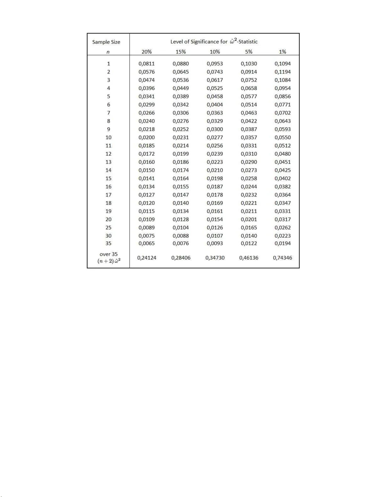
A note on the b est in v arian t estimation of contin uous probabilit y distributions under mean square loss Thomas Sch¨ urmann ∗ J¨ ulich S up er c omputing Centr e, J ¨ ulich R ese ar ch Centr e, 52425 J¨ u li ch, Germany W e consider the nonparametric estimation problem of contin uous probabilit y distribution func- tions. F or the integrated mean squ are error w e p ro vide the statistic corresp onding to the b est inv ariant estimator prop osed by A gga rwal [9] and F erguson [10]. The table of critical v alues is computed and a numerical pow er comparison of the statistic with the traditional Cram´ er-von Mises statistic is done for several representativ e distributions. Keyw ords: Cr am ´ er-von Mises statistic; Goodness of fit criteria; Best in v ariant estimates; Empirical distribu- tion function; Statistical p o wer In 1 933, Kolmogog o v [1] for mally defined the empiri- cal distribution function F n ( x ), and then consider ed how close this w ould b e to the true distribution function F ( x ) when it is con tinuous. This c o n tribution in tro duced the use of F n ( x ) as an estimator of F ( x ), to be follow ed by its use in testing a given F ( x ). Mo difying the statis- tics prop osed earlier by Cram´ er [2] and von Mises [3], Smirnov [4][5] compar ed the hypothesis F ( x ) with F n ( x ) by means of the q ua dratic loss fu nction L = Z ∞ −∞ ( F ( x ) − F n ( x )) 2 w ( F ( x )) dF ( x ) (1) where w is some preassig ned p ositive weigh t function. Let x 1 , ..., x n be a ra ndom sample dr a wn fr o m the con- tin uous probability distribution function F ( x ) with den- sity function f ( x ) and let x ∗ 1 < x ∗ 2 < ... < x ∗ n be obtained by order ing each rea lization x 1 , ..., x n . F or w = 1 , the expression ( 1) can b e written equiv alently as ω 2 = 1 12 n 2 + 1 n n X i =1 h F i − 2 i − 1 2 n i 2 (2) with F i = F ( x ∗ i ). The term nω 2 is commonly named as the Cram´ er-von Mises statistic. Smirnov [4][5][6] showed that the probability distribution o f the latter is indep en- dent o f F for any n and he obtained an asy mptotic e x - pression of its pr o babilit y dis tribution for n → ∞ . F or general weigh t functions , Anderson a nd Darling [7][8] presented a genera l metho d for obtaining the asymptotic distribution of (1) for n → ∞ . Later on, Aggar w al [9] considered a class of in v ariant loss functions a nd obtained the best inv ariant estimators which ar e also step functions like F n ( x ). The canonical representation of a n y in v ariant estimator is given by ˆ F ( x ) = n X i =0 ˆ F i 1 ν i ( x ) (3) with real v alued factors 0 ≤ ˆ F i ≤ 1 , i = 0 , ..., n , and 1 ν i ( x ) is the indica tor function of the s et ν i , which is defined by ν 0 = ( −∞ , x ∗ 1 ) ν i = [ x ∗ i , x ∗ i +1 ) i = 1 , ..., n − 1 , (4) ν n = [ x ∗ n , ∞ ) . Note that for the empirica l distribution, each set ν i is uniquely cor respo nding to the particula r proba bilit y es- timate i/n , for i = 0 , ..., n . F or the ris k function R = E Z ( F − ˆ F ) 2 w ( F ) dF (5) it is known [9][1 0] that ˆ F ( x ) = F n ( x ) (6) is the b est inv aria n t estimate if the weight function is w ( t ) = 1 /t (1 − t ), while the corresp onding statistic (1) is given by A 2 = − 1 − 1 n n X i =1 2 i − 1 n h log F i + log(1 − F n − i +1 ) i . (7) The expression nA 2 is the commonly denoted Anderson- Darling statistic. On the other hand, it is also known that the estimator ˆ F ( x ) = nF n ( x ) + 1 n + 2 (8) is best in v ariant for the ordina r y mean s quare err or with w ( t ) = 1 in (1). Although the la tter can be considered as an improvemen t of the Cram´ er-von Mise s statistic, it app ears that ther e is no explicit expr ession of the co rre- sp onding statistic g iven in literature. Read [11] po in ted out that (6) and (8) can be improv ed by an estimator which is sto c hastically smaller than the Ko lmogorov s ta tistic. How ever, the co rresp onding estimator is not a step function a nd is not inv ariant under the full gr oup o f strictly increasing transfo rma- tions a s are (6) and (8). Another discussion concerns the admissibil ity of the estimators (6) and (8). F or 2 instance, Y u [1 3][14][15] has shown that (6) is admissible with resp ect to the weigh t w ( t ) = 1 /t (1 − t ) only for samples o f s iz e n = 1 , 2 but inadmissible for samples of size n ≥ 3. Similarly , for the estimator (8), Br o wn [1 2] has proven inadmissibility for all sa mple sizes n ≥ 1. Nevertheless, it is not known if the alterna tive estimato r in Brown’s pro of is by itself admissible o r whether it is pos sible to find s o me other estimator do minating (8) which provides a significantly la rger saving in risk from using (8 ). Therefore , let us pr o vide the following: Prop osition 1. F or unit weight w = 1, the s ta tistic (1) corres p onding to the b est in v ariant estimator (8) is ˆ ω 2 = n + 8 12( n + 2) 3 + 1 n + 2 n X i =1 h F i − i + 1 2 n + 2 i 2 . (9) Pro of. T o obta in (9 ) one has to replace F n ( x ) in (1) by the estimator (8) a nd compute the integration. After some algebra ic manipulations expr ession (9) is obtained.  The statistic ˆ ω 2 is similar but differe nt from the traditional Cram´ er-von Mises statistic (2 ). F or large sample sizes they have similar sto c hastic prop erties. The minimum r isk o f the sta tistic is 1 / 6( n + 2), which is slightly less than for the Cr am ´ er -v on Mises statistic with 1 / 6 n . Th us, at lea st for small samples we ca n exp ect that (9) will improve (2). The critical v alues o f (9) are co mputed by numerical simulation and ar e provided in the table of Figure 1. F or n = 1, the cr itical v a lues are 1 / 3 of the critical v alues for the traditional statistic. Mo reov er, fo r the 1 perc en t con- fidence level the critica l v alues are not strictly monotonic decreasing for increa sing sample siz e. W e chec ked that fact by analytica l ev alua tion for n = 1 and 2. All qua n- tiles of the table are sy stematically smaller than for the quantiles of (2). How ever, that does not necessar ily imply that there is an improv ement of the type I e r ror a gainst the Cram´ er-von Mises statistic bec a use for finite sample size n the quantiles of b oth statistics hav e differ e nt sup- po rt and the s cales are no t co mparable. Ther e fo re, we compared their statistical p ow er for a few representative examples of distr ibutions F ( x ), which are supp osed to b e contin uous a nd completely sp e c ified. First, we consider ed the test for norma lit y ( H 0 ), when f ( x ) is the uniform distribution ( H 1 ). In Figure 2 , we see the difference ∆ P of the p ow er of (9) and the p ow er of (2), for co nfidence levels 20 , 1 5 , 10 , 5 and 1 p ercentage po in ts. The numerical simulation has b een p erformed for 1 0 7 Monte Carlo s teps. F or very small and very large samples n , the p o wer of b oth statistics b ecomes mo re and more equal. Int ermedia tely , the difference of the power betw een b oth grows un til 25 percent. F or all sample sizes and confidence levels there is a higher p ow er o f (9) than for the C r am ´ er a nd von Mises statistic. Moreov er, we considere d the tes t for uniformity given in T able 3 o f Stephens study [16]. When F ( x ) is co m- pletely sp ecified then F i should b e uniformly distributed betw een 0 a nd 1. The p o wer study has therefore b e e n confined to a test o f this hypothesis when F i is drawn from alternative distr ibutio ns . If the v ar iance of the hy- po thesized F ( x ) is cor rect but the mea n is wrong, the F i po in ts will tend to mov e tow ar d 0 of 1 ; if the mean is correct but the v ar ia nce is wr ong, the po in ts will mov e to each end, o r will mov e to 1/2 . Acco rdingly , in the Stephens study [16], three v ar ian ts A, B and C hav e b een defined. Case A gives ra ndo m po in ts closer to zero than exp ected o n the hypothesis of unifor mit y ( H 0 ); B gives po in ts near 1/2 ; and C g iv es tw o clusters close to the bo undary 0 and 1. Fir st, w e v erified the table of p ow ers in [16] for the Cr am ´ er - v on Mises statistic and subsequently computed the p ow er of (9) for n = 1 , ..., 40. F or ca se A, we found that b oth hav e very similar p o wer. In case B, the Cram´ er-von Mises statistic is slightly improv ed by (9). Actually for cas e C, there is a significant improve- men t for all sample sizes and all levels o f confidence. The latter is shown in Figure 3. Here, we hav e qua litativ ely the same picture as in Figur e 2. The difference of the power of b oth statis tics is p ositiv e and r eac hes up to 18 per cen tage po in ts. It should b e mentioned her e that for case C, in the Stephens study the Anderson- Da rling statistic is sup e- rior co mpa red to the traditional Cr am ´ er and von Mises statistic. If we compar e the new statistic (9) with the Anderson-Darling sta tis tic for the same ca s e C, then we find that the p ow er of the former is significa ntly higher. This might e nc o urage further inv estigations of (9). ∗ Electronic address: t.sc hurmann@icloud.com [1] Kolmogoro v, A. N. (1933). Sul la determinazione empir- ic a di una le gge di distribuzione, Giorn. Ist. I tal. Attuari 4 , 83-91. [2] Cram ´ er, H. (1928). O n the c omp osition of elementary er- r ors: I I, Statistic al applic ations , Scandin avian Actu arial Journal 11 , 141-180. [3] V on Mises, R. E. ( 1931). Wahrscheinlichkeitsr e chnung und i hr e Anwendung i n der Statistik und the or etischen Physik , Deutick e (Leipzig-Wien, 1931). [4] Smirnov, N. V. (19 36). Sur la di str ibution de ω 2 -criterion (crit ´ erium de M. R. v. Mises), C. R. Acad. Sci. Par is 202 , 449-452. [5] Smirnov, N. V. (1937). On the distribution of the ω 2 - criterion, Math. Sb ornik NS 2 , 973-993. [6] Smirnov, N. V. (1939). On the deviation of the empiric al distribution function, Math. Sb ornik NS 6 , 3-26. [7] Anderson, T. W. and Darling, D. A. (1952). Asymp- totic the ory of c ertain ’Go o dness of Fit’ criteria b ase d on sto chastic pr o c esses, An nals of Mathematical Statistics 23 , 193-212. [8] Anderson, T. W. and Darling, D . A. (1954). A test of Go o dness-of-Fit . Journal of the American Statistical As- 3 sociation 49 , 765-769. [9] Aggarwal , O. P . ( 195 5). Som e minim ax invariant pr o c e- dur es for estimating a cumulative distribution function, Annals of Mathematical Statistics 26 , 450-462. [10] F erguson, T. S . (1967). Mathematic al Statistics: A De- cision The or etic Appr o ach , Academic Press In c., New Y ork. [11] Read, R. R. (1972). The asymptotic i nadmissibility of the sample distribution function, Annals of Mathematical Statistics 43 , 89-95. [12] Brow n, L. D. (19 88). A dmissibili ty in discr ete and c ontin- uous invariant nonp ar ametric estimation pr oblems and in their multinomial analo gs, Annals of Statistics 16 , 1567- 1593. [13] Y u, Q. (1989a). I nadmissibility of the empiric al distribu- tion f unction in c ontinuous i nvariant pr oblems, Annals of Statistics 17 , 1347-1359. [14] Y u, Q. (1989b). A dmissibility of the empiri c al di str ibution function in the invariant pr oblem, Statist. and Decisions 7 , 383-398. [15] Y u, Q. ( 1989c). A dmi ssibi lity of the b est i nvariant esti- mator of a distribution function, Statist. and Decisions 7 , 1-14. [16] Stephens, M. A. (1974). EDF statistics for go o dness of fit and some c omp arisons, Journal of the American S ta- tistical Asso ciation 69 , 730-737. 4 FIG. 1: T able of critical v alues for th e test statistic ˆ ω 2 provided in Prop osition 1. The quantiles are defined b y P ( ˆ ω 2 > Q α ) = α . The asymptotic v alues for n > 35 are giv en by the p ercen tage p oin ts in the last line of t h e table for eve ry confiden ce level. The latter are to b e compared with ( n + 2) ˆ ω 2 . The table is computed by Monte Carlo sim ulations of 5 × 10 7 respective samples. 5 0 10 20 30 40 0 5 10 15 20 25 Sample size n D P FIG. 2: Difference ∆ P for the p ow er of the new statistic (9) and t he traditional Cram ´ er-von Mises statistic (2). The test is for the normal distribution ( H 0 ) against uniform distribution ( H 1 ). Confidence levels are 20, 15, 10, 5, 1 p ercentage p oin ts (from left to right). The Monte Carlo simulatio n is based on 10 7 samples. The erratic b ehavior for very small samples is of systematical nature and not caused by insufficient sampling. 0 10 20 30 40 0 5 10 15 20 Sample size n D P FIG. 3: The same as in Figure 2, excep t that the test is for un ifo rmity (see tex t) correspondin g to Case C of [16]. The confi dence levels are 20, 15, 10, 5, 1 p ercen tage p oin ts (from left to righ t). The Monte Carlo sim ulation is based on 10 7 samples.