A General Distributed Dual Coordinate Optimization Framework for Regularized Loss Minimization

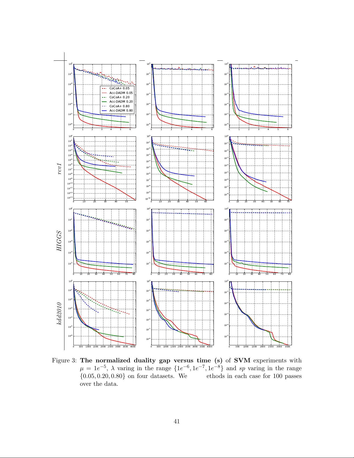
A General Distributed Dual Co ordinate Optimization F ramew ork for Regularized Loss Minimization Sh un Zheng ∗ zhengs14@mails.tsinghua.edu.cn Institute for Inter disciplinary Information Scienc es Tsinghua University Beijing, China Jialei W ang jialei@uchicago.edu Dep artment of Computer Scienc e University of Chic ago Chic ago, Il linois F en Xia xiafen@baidu.com Institute of De ep L e arning Baidu R ese ar ch Beijing, China W ei Xu weixu@tsinghua.edu.cn Institute for Inter disciplinary Information Scienc es Tsinghua University Beijing, China T ong Zhang tongzhang@tongzhang-ml.org T enc ent AI Lab Shenzhen, China Abstract In mo dern large-scale mac hine learning applications, the training data are often parti- tioned and stored on m ultiple mac hines. It is customary to emplo y the “data parallelism” approac h, where the aggregated training loss is minimized without mo ving data across mac hines. In this paper, w e in tro duce a nov el distributed dual form ulation for regularized loss minimization problems that can directly handle data parallelism in the distributed setting. This form ulation allows us to systematically deriv e dual co ordinate optimization pro cedures, whic h w e refer to as Distribute d Alternating Dual Maximization (DADM). The framew ork extends earlier studies describ ed in (Bo yd et al., 2011; Ma et al., 2017; Jaggi et al., 2014; Y ang, 2013) and has rigorous theoretical analyses. Moreov er with the help of the new formulation, we develop the accelerated version of D ADM (Acc-DADM) b y gener- alizing the acceleration tec hnique from (Shalev-Shw artz and Zhang, 2014) to the distributed setting. W e also provide theoretical results for the prop osed accelerated version and the new result improv es previous ones (Y ang, 2013; Ma et al., 2017) whose iteration complex- ities grow linearly on the condition num b er. Our empirical studies v alidate our theory and sho w that our accelerated approach significan tly improv es the previous state-of-the-art distributed dual co ordinate optimization algorithms. Keyw ords: Distributed Optimization, Sto c hastic Dual Co ordinate Ascent, Regularized Loss Minimization ∗ . Most of the work was done during the internship of Sh un Zheng at Baidu Big Data Lab in Beijing. 1 1. In tro duction In large-scale mac hine learning applications for big data analysis, it b ecomes a common practice to partition the training data and store them on m ultiple machines that are con- nected via a commodity net work. A typical setting of distributed machine learning is to allo w these machines to train in parallel, with each machine pro cessing its o wn lo cal data with no data comm unication. This is often referred to as data p ar al lelism . In order to re- duce the ov erall training time, it is often necessary to increase the num b er of mac hines and to minimize the comm unication o verhead. A ma jor c hallenge is to reduce the training time as muc h as p ossible when w e increase the num b er of machines. A practical solution requires t wo researc h directions: one is to impro ve the underlying system design making it suitable for mac hine learning algorithms (Dean and Ghema w at, 2008; Zaharia et al., 2012; Dean et al., 2012; Li et al., 2014); the other is to adapt traditional single-mac hine optimization metho ds to handle data parallelism (Boyd et al., 2011; Y ang, 2013; Maha jan et al., 2013; Shamir et al., 2014; Jaggi et al., 2014; Maha jan et al., 2014; Ma et al., 2017; T ak´ a ˇ c et al., 2015; Zhang and Lin, 2015). This pap er fo cuses on the latter. F or big data mac hine learning on a single machine, there are generally tw o t yp es of algorithms: batc h algorithms suc h as gradien t descent or L-BFGS (Liu and No cedal, 1989), and stochastic optimization algorithms such as sto c hastic gradien t descen t and their modern v ariance reduced v ersions (Defazio et al., 2014; Johnson and Zhang , 2013). It is known that batc h algorithms are relatively easy to parallelize. Ho wev er, on a single mac hine, they con verge more slowly than the mo dern stochastic optimization algorithms due to their high p er-iteration computation costs. Specifically , it has b een shown that the mo dern sto c hastic optimization algorithms con verge faster than the traditional batc h algorithms for con v ex regularized loss minimization problems. The faster con vergence can b e guaran teed in theory and observed in practice. The fast conv ergence of modern sto c hastic optimization metho ds has led to studies to ex- tend these metho ds to the distributed computing setting. Specifically , this pap er considers the generalization of Sto c hastic Dual Co ordinate Ascent metho d (Hsieh et al., 2008; Shalev- Sh wartz and Zhang, 2013) and its pro ximal v ariant (Shalev-Shw artz and Zhang, 2014) to handle distributed training using data parallelism. Although this problem has b een consid- ered previously (Y ang, 2013; Jaggi et al., 2014; Ma et al., 2017), these earlier approac hes w ork with the dual form ulation that is the same as the traditional single-machine dual for- m ulation, where dual v ariables are coupled, and hence run into difficulties when they try to motiv ate and analyze the deriv ed metho ds under the distributed environmen t. A ma jor con tribution of this w ork is to introduce a new dual form ulation sp ecifically for distributed regularized loss minimization problems when data are distributed to multiple mac hines. In our new form ulation, we decouple the lo cal dual v ariables through introducing another dual v ariable β . This new dual form ulation allows us to naturally extend the pro x- imal SDCA algorithm (ProxSDCA) of (Shalev-Shw artz and Zhang, 2014) to the setting of m ulti-machine distributed optimization that can benefit from data parallelism. Moreo ver, the analysis of the original Pro xSDCA can b e easily adapted to the new formulation, lead- ing to new theoretical results. This new dual formulation can also b e com bined with the acceleration tec hnique of (Shalev-Sh wartz and Zhang, 2014) to further impro ve conv ergence. 2 In the prop osed form ulation, each iteration of the distributed dual co ordinate ascent optimization is naturally decomp osed in to a lo cal step and a global step. In the local step, w e allo w the use of any lo cal pro cedure to optimize a local dual ob jective function using lo cal parameters and lo cal data on each machine. This flexibility is similar to those of (Ma et al., 2017; Jaggi et al., 2014). F or example, we ma y apply Pro xSDCA as the lo cal procedure. In the local step, a computer no de can p erform the optimization indep enden tly without comm unicating with each other. While in the global step, no des comm unicate with each other to synchronize the lo cal parameters and jointly up date the global primal solution. Only this global step requires communication among no des. W e summarize our main contributions as follows: New distributed dual form ulation This new form ulation naturally leads to a tw o step lo cal-global dual alternating optimization procedure for distributed mac hine learning. W e th us call the resulting pro cedure Distribute d A lternating Dual Maximization (D ADM). Note that DADM directly generalizes ProxSDCA, whic h can handle complex regularizations such as L 2 - L 1 regularization. New con vergence analysis The new form ulation allo ws us to directly generalize the analysis of ProxSDCA in (Shalev-Shw artz and Zhang, 2014) to the distributed setting. This is in con trast to that of CoCoA + in (Ma et al., 2017), whic h employs a differen t analysis based on the Θ-approximate solution assumption of the lo cal solver. Our analysis can lead to simplified results in the commonly used mini-batch setup. Acceleration with theoretical guarantees Based on the new distributed dual formu- lation, w e can naturally derive a distributed version of the accelerated pro ximal SDCA metho d (AccProxSDCA) of (Shalev-Shw artz and Zhang, 2014), whic h has been shown to b e effectiv e on a single mac hine. W e call the resulting pro cedure A c c eler ate d Distribute d A lternating Dual Maximization (Acc-D ADM). The main idea is to mo dify the original for- m ulation using a sequence of appro ximations that hav e stronger regularizations. Moreo ver W e directly adapt theoretical analyses of AccProxSDCA to the distributed setting and pro vide guaran tees for Acc-D ADM. Our theorem guarantees that we can alw ays obtain a computation sp eedup compared with the single-mac hine AccPro xSDCA. This impro v es the theoretical results of D ADM and previous metho ds (Y ang, 2013; Ma et al., 2017) whose iteration complexities gro w linearly on the condition num ber, and latter metho ds p ossibly fail to pro vide computation time impro vemen t ov er the single-mac hine Pro xSDCA when the condition num b er is large. Extensiv e empirical studies W e p erform extensive exp eriments to compare the conv er- gence and the scalability of the accelerated approach with that of previous state-of-the-art distributed dual coordinate ascen t metho ds. Our empirical studies show that Acc-DADM can achiev e faster conv ergence and b etter scalabilit y than previous state-of-the-arts, in par- ticular when the condition n umber is relativ ely large. This phenomenon is consisten t with our theory . W e organize the rest of the pap er as follows. Section 2 discusses related w orks. Section 3 pro vides preliminary definitions. Section 4 to 6 presen t the distributed primal formula- tion, the distributed dual form ulation and our DADM method resp ectiv ely . Section 7 then pro vides theorems for D ADM. Section 8 introduces the accelerated v ersion and pro vides 3 corresp onding theoretical guarantees. Section 9 includes all pro ofs of this pap er. Section 10 pro vides extensiv e empirical studies of our nov el metho d. Finally , Section 11 concludes the whole pap er. 2. Related W ork Sev eral generalizations of SDCA to the distributed settings ha ve b een prop osed in the literature, including DisDCA (Y ang, 2013), CoCoA (Jaggi et al., 2014), and CoCoA + (Ma et al., 2017). DisDCA was the first attempt to study distributed SDCA, and it pro vided a basic theoretical analysis and a practical v arian t that b eha ves well empirically . Nev ertheless, their theoretical result only applies to a few sp ecially c hosen mini-batc h lo cal dual up dates that differ from the practical method used in their exp erimen ts. In particular, they did not sho w that optimizing eac h lo cal dual problem leads to con vergence. This limitation makes the metho ds they analyzed inflexible. CoCoA was prop osed to fix the ab o v e gap b etw een theory and practice, and it was claimed to b e a framework for distributed dual coordinate ascen t in that it allows an y local dual solver to be used for the lo cal dual problem, rather than the impractical c hoices of DisDCA. How ever, the practical p erformance of CoCoA is inferior to the practical v arian t prop osed in DisDCA with an aggressiv e lo cal update. W e note that the practical v ariant of DisDCA did not hav e a solid theoretical guarantee at that time. CoCoA + fixed this situation and ma y b e regarded as a generalization of CoCoA. The most effectiv e c hoice of the aggregation parameter leads to a version which is similar to DisDCA, but allo ws exact optimization of eac h dual problem in their theory . According to studies in (Ma et al., 2017), the resulting CoCoA + algorithm p erforms significantly b etter than the original CoCoA b oth theoretically and empirically . The original CoCoA + (Ma et al., 2015) can only handle problems with the L 2 regularizer and it was generalized to general strongly con vex regularizers in the long version (Ma et al., 2017). Besides (Smith et al., 2016) extended the framew ork to solv e the primal problem of regularized loss min- imization and cov er general non-strongly conv ex regularizers suc h as L 1 regularizer, and (Hsieh et al., 2015) studied parallel SDCA with asynchronous updates. Although CoCoA + has the adv antage of allowing arbitrary lo cal solvers and flexible appro ximate solutions of lo cal dual problems, its theoretical analyses do not capture the con tribution of the n um b er of mac hines and the mini-batc h size to the iteration complexity explicitly . Moreov er the iteration complexities of b oth CoCoA + and DisDCA grow linearly with the condition n um b er, th us they probably cannot pro vide computation time impro ve- men t o v er the single-machine SDCA when the condition n umber is large. This pap er will remedy these unsatisfied asp ects by providing a different analysis based on a new distributed dual formulation. Using this formulation, we can analyze pro cedures that can tak e an ar- bitrary local dual solv er, which is like CoCoA + ; moreo ver, we allo w the dual up dates to be a mini-batch, which is like DisDCA. Moreov er this formulation also allows us to naturally generalize AccProxSDCA and relev ant theoretical results to the distributed setting. Our empirical results also v alidate the sup eriorit y of the accelerated approach. While we focus on extending SDCA in this pap er, we note that there are other ap- proac hes for parallel optimization. F or example, there are direct attempts to parallelize 4 sto c hastic gradient descent (Rech t et al., 2011; Zinkevic h et al., 2010). Some of these pro- cedures only consider multi-core shared memory situation, whic h is very different from the distributed computing environmen t in v estigated in this pap er. In the setting of dis- tributed computing, data are partitioned in to multiple mac hines and one often needs to study comm unication-efficient algorithms. In suc h cases, one extreme is to allow exact opti- mization of subproblems on each lo cal machine as considered in (Shamir et al., 2014; Zhang and Lin, 2015). Although this approac h minimizes comm unication, the computational cost for each lo cal solver can dominate the o v erall training. Therefore in practice, it is necessary to do a trade-off b y using the mini-batc h update approac h (T ak ac et al., 2013; T ak´ aˇ c et al., 2015). How ever, it is difficult for traditional mini-batch metho ds to design reasonable ag- gregation strategies to ac hiev e fast conv ergence. (T ak´ a ˇ c et al., 2015) studied ho w the step size can be reduced when the mini-batch size grows in the distributed setting. (Lee and Roth, 2015) derived an analytical solution of the optimal step size for dual linear supp ort v ector mac hine problems. Besides (Maha jan et al., 2013) presented a general framew ork for distributed optimization based on lo cal functional appro ximation, whic h include several first-order and second-order metho ds as sp ecial cases, and (Maha jan et al., 2014) considered eac h machine to handle a block of co ordinates, and prop osed distributed blo c k co ordinate descen t metho ds for solving ℓ 1 regularized loss minimization problems. Differen t from those metho ds, Distribute d Alternating Dual Maximization (D ADM) pro- p osed in this work handles the trade-off b et ween computation and comm unication b y de- v eloping b ounds for mini-batch dual up dates, which is similar to (Y ang, 2013). Moreo v er, D ADM allows other b etter lo cal solvers to ac hieve faster con vergence in practice. 3. Preliminaries In this section, w e in tro duce some notations used in the follo wing section. All functions that we consider in this pap er are prop er con vex functions o ver a Euclidean space. Giv en a function f : R d → R , w e denote its conjugate function as f ∗ ( b ) = sup a [ b ⊤ a − f ( a )] . A function f : R d → R is L -Lipsc hitz with resp ect to ∥ · ∥ 2 if for all a, b ∈ R d , w e hav e | f ( a ) − f ( b ) | ≤ L ∥ a − b ∥ 2 . A function f : R d → R is (1 /γ ) -smo oth with resp ect to ∥ · ∥ 2 if it is differentiable and its gradien t is (1 /γ )-Lipsc hitz with resp ect to ∥ · ∥ 2 . An equiv alen t definition is that for all a, b ∈ R d , we ha v e f ( b ) ≤ f ( a ) + ∇ f ( a ) ⊤ ( b − a ) + 1 2 γ ∥ b − a ∥ 2 2 . A function f : R d → R is λ -strongly conv ex with resp ect to ∥ · ∥ 2 if for an y a, b ∈ R d , w e hav e f ( b ) ≥ f ( a ) + ∇ f ( a ) ⊤ ( b − a ) + λ 2 ∥ b − a ∥ 2 2 , where ∇ f ( a ) is any subgradien t of f ( a ). It is w ell kno wn that a function f is γ -strongly con v ex with resp ect to ∥ · ∥ 2 if and only if its conjugate function f ∗ is (1 /γ )-smo oth with resp ect to ∥ · ∥ 2 . 5 4. Distributed Primal F ormulation In this pap er, w e consider the following generic regularized loss minimization problem: min w ∈ R d  P ( w ) := n  i =1 ϕ i ( X ⊤ i w ) + λng ( w ) + h ( w )  , (1) whic h is often encoun tered in practical machine learning problems. Here we assume each X i ∈ R d × q is a d × q matrix, w ∈ R d is the model parameter vector, ϕ i ( u ) is a con vex loss function defined on R q , which is asso ciated with the i -th data p oin t, λ > 0 is the regularization parameter, g ( w ) is a strongly conv ex regularizer and h ( w ) is another conv ex regularizer. A special case is to simply set h ( w ) = 0. Here w e allow the more general form ulation, whic h can b e used to derive different distributed dual forms that ma y b e useful for sp ecial purp oses. The abov e optimization form ulation can be sp ecialized to a v ariety of machine learning problems. As an example, w e ma y consider the L 2 - L 1 regularized least squares problem, where ϕ i ( x ⊤ i w ) = ( w ⊤ x i − y i ) 2 for vector input data x i ∈ R d and real v alued output y i ∈ R , g ( w ) = ∥ w ∥ 2 2 + a ∥ w ∥ 1 , and h ( w ) = b ∥ w ∥ 1 for some a, b ≥ 0. If we set h ( w ) = 0, then it is well-kno wn (see, for example, (Shalev-Shw artz and Zhang, 2014)) that the primal problem (1) has an equiv alen t single-machine dual form of max α ∈ R n  D ( α ) := − n  i =1 ϕ ∗ i ( − α i ) − λng ∗   n i =1 X i α i λn   , (2) where α = [ α 1 , · · · , α n ] , α i ∈ R q ( i = 1 , ..., n ) are dual v ariables, ϕ ∗ i is the conv ex conjugate function of ϕ i , and similarly , g ∗ is the conv ex conjugate function of g . The stochastic dual co ordinate ascent metho d, referred to as SDCA in (Shalev-Shw artz and Zhang, 2014), maximizes the dual formulation (2) by optimizing one randomly c ho- sen dual v ariable at each iteration. Throughout the algorithm, the follo wing primal-dual relationship is maintained: w ( α ) = ∇ g ∗   n i =1 X i α i λn  , (3) for some subgradient ∇ g ∗ ( v ). It is known that w ( α ∗ ) = w ∗ , where w ∗ and α ∗ are optimal solutions of the primal problem and the dual problem resp ectively . It was shown in (Shalev-Sh wartz and Zhang, 2014) that the dualit y gap defined as P ( w ( α )) − D ( α ), whic h is an upp er-b ound of the primal sub-optimality P ( w ( α )) − P ( w ∗ ), con v erges to zero. Moreov er, a con v ergence rate can b e established. In particular, for smo oth loss functions, the conv ergence rate is linear. W e note that SDCA is suitable for optimization on a single mac hine due to the fact that it works with a dual formulation that is suitable for a single machine. In the follo wing, w e will generalize the single-machine dual form ulation (2) to the distributed setting, and study the corresp onding distributed v ersion of SDCA. In the distributed setting, we assume that the training data are partitioned and dis- tributed to m mac hines. In other w ords, the index set S = { 1 , ..., n } of the training data is divided in to m non-ov erlapping partitions, where each machine ℓ ∈ { 1 , ..., m } contains its 6 o wn partition S ℓ ⊆ S . W e assume that ∪ ℓ S ℓ = S , and w e use n ℓ := | S ℓ | to denote the size of the training data on machine ℓ . Next, we can rewrite the primal problem (1) as the following constrained minimization problem that is suitable for the multi-mac hine distributed setting: min w ; { w ℓ } m ℓ =1 m  ℓ =1 P ℓ ( w ℓ ) + h ( w ) s.t. w ℓ = w, for all ℓ ∈ { 1 , ..., m } , where P ℓ ( w ℓ ) :=  i ∈ S ℓ ϕ i ( X ⊤ i w ℓ ) + λn ℓ g ( w ℓ ) , (4) where w ℓ represen ts the lo cal primal v ariable on eac h machine ℓ , P ℓ is the corresp onding lo cal primal problem and the constraints w ℓ = w are imp osed to synchronize the local primal v ariables. Obviously this m ulti-mac hine distributed primal formulation (4) is equiv alent to the original primal problem (1). W e note that the idea of ob jectiv e splitting in (4) is similar to the global v ariable con- sensus form ulation describ ed in (Boyd et al., 2011). Instead of using the commonly used ADMM (Alternating Direction Metho d of Multipliers) metho d that is not a generalization of (2), in this paper w e deriv e a distributed dual form ulation based on (4) that directly generalizes (2). W e further propose a framew ork called Distributed Alternating Dual Max- imization (D ADM) to solv e the distributed dual form ulation. One adv antage of DADM o ver ADMM is that D ADM do es not need to solve the subproblems in high accuracy , and th us it can naturally enjo y the trade-off betw een computation and comm unication, whic h is similar to related metho ds such as DisDCA, CoCoA and CoCoA + . 5. Distributed Dual F ormulation The optimization problem (4) can b e further rewritten as: min w ; { w ℓ } ; { u i } m  ℓ =1    i ∈ S ℓ ϕ i ( u i ) + λn ℓ g ( w ℓ )   + h ( w ) s.t u i = X ⊤ i w ℓ , for all i ∈ S ℓ w ℓ = w, for all ℓ ∈ { 1 , ..., m } . (5) Here we introduce n dual v ariables α := { α i } n i =1 , where each α i is the Lagrange multiplier for the constraint u i − X ⊤ i w ℓ = 0, and m dual v ariables β := { β ℓ } m ℓ =1 , where each β ℓ is the Lagrange multiplier for the constraint w ℓ − w = 0. W e can now introduce the primal-dual ob jective function with Lagrange multipliers as follo ws: J ( w ; { w ℓ } ; { u i } ; { α i } ; { β ℓ } ) := m  ℓ =1    i ∈ S ℓ  ϕ i ( u i ) + α ⊤ i ( u i − X ⊤ i w ℓ )  + λn ℓ g ( w ℓ ) + β ⊤ ℓ ( w ℓ − w )   + h ( w ) . 7 Prop osition 1 Define the dual obje ctive as D ( α, β ) := m  ℓ =1    i ∈ S ℓ − ϕ ∗ i ( − α i ) − λn ℓ g ∗   i ∈ S ℓ X i α i − β ℓ λn ℓ    − h ∗   ℓ β ℓ  . Then we have D ( α, β ) = min w ; { w ℓ } ; { u i } J ( w ; { w ℓ } ; { u i } ; { α i } ; { β ℓ } ) , wher e the minimizers ar e achieve d when the fol lowing e quations ar e satisfie d ∇ ϕ i ( u i ) + α i =0 , −    i ∈ S ℓ X i α i − β ℓ   + λn ℓ ∇ g ( w ℓ ) =0 , −  ℓ β ℓ + ∇ h ( w ) =0 , (6) for some sub gr adients ∇ ϕ i ( u i ) , ∇ g ( w ℓ ) , and ∇ h ( w ) . When β = { β ℓ } are fixed, w e may define the lo cal single-mac hine dual formulation on eac h machine ℓ with resp ect to α ( ℓ ) as ˜ D ℓ ( α ( ℓ ) | β ℓ ) :=  i ∈ S ℓ − ϕ ∗ i ( − α i ) − λn ℓ g ∗   i ∈ S ℓ X i α i − β ℓ λn ℓ  , (7) where α ( ℓ ) represen ts local dual v ariables { α i ; i ∈ S ℓ } on mac hine ℓ , β ℓ ∈ R d serv es as a carrier for sync hronization of mac hine ℓ . Based on Proposition 1, we obtain the follo wing m ulti-machine distributed dual formulation for the corresp onding primal problem (4): D ( α, β ) = m  ℓ =1 ˜ D ℓ ( α ( ℓ ) | β ℓ ) − h ∗  m  ℓ =1 β ℓ  . (8) Moreo ver we hav e the non-negative duality gap, and zero dualit y gap can be ac hieved when w is the minimizer of P ( w ) and ( α, β ) maximizes the dual D ( α, β ). Prop osition 2 Given any ( w, α, β ) , the fol lowing duality gap is non-ne gative: P ( w ) − D ( α, β ) ≥ 0 . Mor e over, zer o duality gap c an b e achieve d at ( w ∗ , α ∗ , β ∗ ) , wher e w ∗ is the minimizer of P ( w ) and ( α ∗ , β ∗ ) is a maximizer of D ( α, β ) . W e note that the parameters { β ℓ } m ℓ =1 pass the global information across multiple ma- c hines. When β ℓ is fixed, ˜ D ℓ ( α ( ℓ ) | β ℓ ) with resp ect to α ( ℓ ) corresp onds to the dual of the adjusted lo cal primal problem: ˜ P ℓ ( w ℓ | β ℓ ) :=  i ∈ S ℓ ϕ i ( X ⊤ i w ℓ ) + λn ℓ ˜ g ℓ ( w ℓ ) , (9) 8 where the original regularizer λn ℓ g ( w ℓ ) in P ℓ ( w ℓ ) is replaced by the adjusted regularizer λn ℓ ˜ g ℓ ( w ℓ ) := λn ℓ g ( w ℓ ) + β ⊤ ℓ w ℓ . Similar to the single-machine primal-dual relationship of (3), we hav e the follo wing lo cal primal-dual relationship on each mac hine as: w ℓ ( α ( ℓ ) , β ℓ ) = ∇ g ∗ ( ˜ v ℓ ) = ∇ ˜ g ∗ ℓ ( v ℓ ) , (10) where v ℓ =  i ∈ S ℓ X i α i λn ℓ , ˜ v ℓ = v ℓ − β ℓ λn ℓ . Moreo ver, w e can define the global primal-dual relationship as w ( α, β ) = ∇ g ∗ ( ˜ v ) = ∇ ˜ g ∗ ( v ) , (11) where v =  n i =1 X i α i λn , ˜ v = v −  ℓ β ℓ λn . W e can also establish the relationship of global-lo cal duality in Proposition 3. Prop osition 3 Given ( w , α, β ) and { w ℓ } such that w 1 = · · · = w m = w , we have the fol lowing de c omp osition of glob al duality gap as the sum of lo c al duality gaps: P ( w ) − D ( α, β ) ≥ m  ℓ =1  ˜ P ℓ ( w ℓ | β ℓ ) − ˜ D ℓ ( α ( ℓ ) | β ℓ )  , and the e quality holds when ∇ h ( w ) =  ℓ β ℓ for some sub gr adient ∇ h ( w ) . Although w e allo w arbitrary h ( w ), the case of h ( w ) = 0 is of special interests. This corresp onds to the conjugate function h ∗ ( β ) =  + ∞ if β  = 0 0 if β = 0 . That is, the term h ∗ (  m ℓ =1 β ℓ ) is equiv alen t to imp osing the constrain t  m ℓ =1 β ℓ = 0. 6. Distributed Alternating Dual Maximization Minimizing the primal formulation (4) is equiv alent to maximizing the dual formulation (8), and the latter can be ac hieved by rep eatedly using the following alternating optimization strategy , which w e refer to as D istributed A lternating D ual M aximization ( DADM ): • Lo cal step : fix β ℓ and let eac h mac hine approximately optimize ˜ D ℓ ( α ( ℓ ) | β ℓ ) w.r.t α ( ℓ ) in parallel. • Global step : maximize the global dual ob jectiv e w.r.t β ℓ , and set the global primal parameter w accordingly . 9 Algorithm 1 Lo cal Dual Up date Retriev e lo cal parameters ( α ( t − 1) ℓ , ˜ v ( t − 1) ℓ ) Randomly pick a mini-batc h Q ℓ ⊂ S ℓ Appro ximately maximize (12) w.r.t ∆ α Q ℓ Up date α ( t ) i as α ( t ) i = α ( t − 1) i + ∆ α i for all i ∈ Q ℓ return ∆ v ( t ) ℓ = 1 λn ℓ  i ∈ Q ℓ X i ∆ α i The ab o ve steps are applied in iterations t = 1 , 2 , . . . , T . A t the b eginning of each iteration t , we assume that the lo cal primal and dual v ariables on eac h local mac hine are ( α ( t − 1) ( ℓ ) , β ( t − 1) ℓ , v ( t − 1) ℓ ), then we seek to up date α ( t − 1) ( ℓ ) to α ( t ) ( ℓ ) and v ( t − 1) ℓ to v ( t ) ℓ in the lo cal step, and seek to up date β ( t − 1) ℓ to β ( t ) ℓ in the global step. W e note that the lo cal step can be executed in parallel w.r.t dual v ariables { α ( ℓ ) } m ℓ =1 . In practice, it is often useful to optimize (7) approximately b y using a randomly selected mini-batc h Q ℓ ⊂ S ℓ of size | Q ℓ | = M ℓ . That is, we w an t to find ∆ α ( t ) i with i ∈ Q ℓ to appro ximately maximize the lo cal dual ob jective as follo ws: ˜ D ( t ) Q ℓ (∆ α Q ℓ ) := −  i ∈ Q ℓ ϕ ∗ i ( − α ( t − 1) i − ∆ α i ) − λn ℓ g ∗  ˜ v ( t − 1) ℓ +  i ∈ Q ℓ X i ∆ α i λn ℓ  . (12) This step is described in Algorithm 1. W e can use any solver for this approximate optimization, and in our exp eriments, w e choose ProxSDCA. The global step is to sync hronize all lo cal solutions, which requires comm unication among the machines. This is achiev ed b y optimizing the following dual ob jective with resp ect to all β = { β ℓ } : β ( t ) ∈ arg max β D ( α ( t ) , β ) . (13) Prop osition 4 Given v , let w ( v ) b e the unique solution of the fol lowing optimization pr ob- lem w ( v ) = arg min w  − λnw ⊤ v + λng ( w ) + h ( w )  (14) that satisfies λn ∇ g ( w ) + ∇ h ( w ) = λnv for some sub gr adients ∇ g ( w ) and ∇ h ( w ) = ρ at w = w ( v ) . Then ¯ β ( v ) = ρ is a solution of max b  − λng ∗  v − b λn  − h ∗ ( b )  , and w ( v ) = ∇ g ∗  v − ¯ β ( v ) λn  . 10 Prop osition 5 Given α , a solution of max β D ( α, β ) c an b e obtaine d by setting β ℓ = λn ℓ  v ℓ ( α ( ℓ ) ) − v ( α ) + ¯ β ( v ( α )) λn  wher e ¯ β ( v ( α )) is define d in Pr op osition 4, v ( α ) =  n i =1 X i α i λn , v ℓ ( α ( ℓ ) ) =  i ∈ S ℓ X i α i λn ℓ . Mor e over, if we let w = w ( α, β ) = w ( v ( α )) = ∇ g ∗  v ( α ) − ¯ β ( v ( α )) λn  , wher e w ( v ) is define d in Pr op osition 4, and w ℓ = w ℓ ( α ( ℓ ) , β ℓ ) = ∇ g ∗  v ℓ ( α ( ℓ ) ) − β ℓ λn ℓ  , then w = w ℓ for al l ℓ , and P ( w ) − D ( α, β ) = m  ℓ =1 [ ˜ P ℓ ( w ℓ | β ℓ ) − ˜ D ℓ ( α ( ℓ ) | β ℓ )] . According to Prop osition 5, the solution of (13) is given b y β ( t ) ℓ = λn ℓ  v ( t ) ℓ − v ( t ) + ρ ( t ) λn  , where v ( t ) = m  ℓ =1 n ℓ n v ( t ) ℓ = v ( t − 1) + m  ℓ =1 n ℓ n ∆ v ( t ) ℓ , and ρ ( t ) = ∇ h ( w ( t ) ) is a subgradient of h at the solution w ( t ) of w ( t ) = arg min w  − λnw ⊤ v ( t ) + λng ( w ) + h ( w )  , that can achiev e the first order optimality condition − λnv ( t ) + λn ∇ g ( w ( t ) ) + ρ ( t ) = 0 for some subgradient ∇ g ( w ( t ) ). 11 Algorithm 2 Distributed Alternating Dual Maximization (DADM) Input: Ob jectiv e P ( w ), target duality gap ϵ , warm start v ariables w init , α init , β init , v init , (if not sp ecified, set w init = 0 , α init = 0 , β init = 0 , v init = 0), . Initialize: let w (0) = w init , α (0) = α init , β (0) = β init , v (0) = v init . for t = 1 , 2 , ... do ( Lo cal step ) for all mac hines ℓ = 1 , 2 , ..., m in parallel do call an arbitrary lo cal pro cedure, such as Algorithm 1 end for ( Global step ) Aggregate v ( t ) = v ( t − 1) +  m ℓ =1 n ℓ n ∆ v ( t ) ℓ Compute ˜ v ( t ) according to (15) Let ∆ ˜ v ( t ) = ˜ v ( t ) − ˜ v ( t − 1) for all mac hines ℓ = 1 , 2 , ..., m in parallel do up date lo cal parameter ˜ v ( t ) ℓ = ˜ v ( t − 1) ℓ + ∆ ˜ v ( t ) end for Stopping condition : Stop if P ( w ( t ) ) − D ( α ( t ) , β ( t ) ) ≤ ϵ . end for return w ( t ) = ∇ g ∗ ( ˜ v ( t ) ), α ( t ) , β ( t ) , v ( t ) , and the duality gap P ( w ( t ) ) − D ( α ( t ) , β ( t ) ). The definition of ˜ v implies that after each global update, we ha v e ˜ v ( t ) ℓ = ˜ v ( t ) = v ( t ) − ρ ( t ) λn = ∇ g ( w ( t ) ) , for all ℓ = 1 , . . . , m. (15) Since the ob jective (12) for the lo cal step on eac h mac hine only dep ends on the mini- batc h Q ℓ (sampled from S ℓ ) and the v ector ˜ v ( t ) ℓ , whic h needs to b e synchronized at eac h global step, w e know from (15) that at each time t , w e can pass the same v ector ˜ v ( t ) as ˜ v ( t ) ℓ to all no des. In practice, it may b e b eneficial to pass ∆ ˜ v ( t ) instead, esp ecially when ∆ ˜ v ( t ) is sparse but ˜ v ( t ) is dense. Put things together, the local-global DADM iterations can b e summarized in Algorithm 2. If we consider the sp ecial case of h ( w ) = 0, the solution of (15) is simply ˜ v ( t ) ℓ = ˜ v ( t ) = v ( t ) , and the global step in Algorithm 2 can b e simplified as first aggregating up dates by ∆ ˜ v ( t ) = ∆ v ( t ) = m  ℓ =1 n ℓ n ∆ v ( t ) ℓ , and then updating lo cal parameters in parallel. F urther, if h ( w ) = 0 and the data partition is balanced, that is n ℓ are iden tical for all ℓ = 1 , . . . , m , it can b e verified that the DADM pro cedure (ignoring the mini-batc h v ariation) is equiv alen t to CoCoA + . Therefore the framew ork presented here may be regarded as an alternative in terpretation. Moreo ver, when the added regularization in (1) is complex and might inv olves more than one non-smo oth term, considering the splitting of g ( w ) and h ( w ) can bring computational adv antages. F or example, to promote b oth sparsity and group sparsity in the predictor we 12 often use the sparse group lasso regularization (F riedman et al., 2010), where a combination of L 1 norm and mixed L 2 /L 1 norm (group sparse norm) is introduced: λ 1  G ∥ w G ∥ 2 + λ 2 ∥ w ∥ 1 + λ 3 / 2 ∥ w ∥ 2 2 , where we add a sligh t L 2 regularization to mak e it strongly con v ex, as did in (Shalev-Sh w artz and Zhang, 2014). The pro ximal mapping with respect to the sparse group lasso regularization function does not hav e closed form solution, thus often relies on iterativ e minimization steps, but there are closed form proximal mapping with resp ect to either L 2 - L 1 norm or the group norm. Th us if we simply set h ( w ) = 0 and λg ( w ) = λ 1  G ∥ w G ∥ 2 + λ 2 ∥ w ∥ 1 + λ 3 / 2 ∥ w ∥ 2 2 , then b oth the lo cal optimization up date (12) and global sync hronization step (14) will not ha v e closed form solution. Ho w ever, if w e assign the group norm on h ( w ) such that h ( w ) = λ 1  G ∥ w G ∥ 2 , and hence λg ( w ) = λ 2 ∥ w ∥ 1 + λ 3 / 2 ∥ w ∥ 2 2 , the lo cal up dates steps (12) will enjoy closed form up date, which mak es the implemen tation muc h easier and w e only need to use iterative minimization on the (rare) global synchronization step (14). 7. Con v ergence Analysis Let w ∗ b e the optimal solution for the primal problem P ( w ) and ( α ∗ , β ∗ ) be the optimal solution for the dual problem D ( α, β ) resp ectiv ely . F or the primal solution w ( t ) and the dual solution ( α ( t ) , β ( t ) ) at iteration t , we define the primal sub-optimalit y as ϵ ( t ) P := P ( w ( t ) ) − P ( w ∗ ) , and the dual sub-optimalit y as ϵ ( t ) D := D ( α ∗ , β ∗ ) − D ( α ( t ) , β ( t ) ) . Due to the close relationship of the distributed dual formulation and the single-machine dual form ulation, an analysis of D ADM can b e obtained by directly generalizing that of SDCA. W e consider tw o kinds of loss functions, smooth loss functions that imply fast linear con vergence and general L -Lipschitz loss functions. F or the following tw o theorems we alw ays assume that g is 1-strongly con vex w.r.t ∥ · ∥ 2 , ∥ X i ∥ 2 2 ≤ R for all i , M ℓ = | Q ℓ | is fixed on each machine, and our lo cal pro cedure optimizes ˜ D ( t ) Q ℓ sufficien tly w ell on eac h mac hine suc h that ˜ D ( t ) Q ℓ (∆ α Q ℓ ) ≥ ˜ D ( t ) Q ℓ (∆ ˜ α Q ℓ ), where ∆ ˜ α Q ℓ is giv en by a sp ecial c hoice in eac h theorem. Theorem 6 Assume that e ach ϕ i is (1 /γ ) -smo oth w.r.t ∥ · ∥ 2 and ∆ ˜ α Q ℓ is given by ∆ ˜ α i := s ℓ ( u ( t − 1) i − α ( t − 1) i ) , for al l i ∈ Q ℓ , wher e u ( t − 1) i := −∇ ϕ i ( X ⊤ i w ( t − 1) ℓ ) and s ℓ := γ λn ℓ γ λn ℓ + M ℓ R ∈ [0 , 1] . T o r e ach an exp e cte d duality gap of E [ P ( w ( T ) ) − D ( α ( T ) , β ( T ) )] ≤ ϵ , every T satisfying the fol lowing c ondition is sufficient, T ≥  R γ λ + max ℓ n ℓ M ℓ  log   R γ λ + max ℓ n ℓ M ℓ  · ϵ (0) D ϵ  . (16) 13 Theorem 7 Assume that e ach ϕ i is L -Lipschitz w.r.t ∥ · ∥ 2 , and ∆ ˜ α Q ℓ is given by ∆ ˜ α i := q n ℓ M ℓ ( u ( t − 1) i − α ( t − 1) i ) , for al l i ∈ Q ℓ , wher e − u ( t − 1) i := ∇ ϕ i ( X ⊤ i w ( t − 1) ℓ ) and q ∈ [0 , min ℓ ( M ℓ /n ℓ )] . T o r e ach an exp e cte d nor- malize d duality gap of E  P ( w ) − D ( α,β ) n  ≤ ϵ , every T satisfying the fol lowing c ondition is sufficient, T ≥ T 0 + max  ˜ n, G λϵ  , (17) T 0 ≥ max  t 0 , 4 G λϵ − 2 ˜ n + t 0  , (18) t 0 = max  0 , ⌈ ˜ n log(2 λ ˜ n ϵ (0) D nG ) ⌉  , (19) wher e ˜ n = max ℓ ( n ℓ / M ℓ ) , G = 4 R L 2 and w, α, β r epr esent either the aver age ve ctor or a r andomly chosen ve ctor of w ( t − 1) , α ( t − 1) , β ( t − 1) over t ∈ { T 0 + 1 , ..., T } r esp e ctively, such as α = 1 T − T 0  T t = T 0 +1 α ( t − 1) , β = 1 T − T 0  T t = T 0 +1 β ( t − 1) , w = 1 T − T 0  T t = T 0 +1 w ( t − 1) . Remark 8 Both The or em 6 and The or em 7 inc orp or ate two key c omp onents: the term max ℓ n ℓ M ℓ and the c ondition numb er term 1 λγ or L 2 λ . When the iter ation c omplexity is domi- nate d by the term max ℓ n ℓ M ℓ , we c an sp e e d up c onver genc e and r e duc e the numb er of c ommu- nic ations by incr e asing the numb er of machines m or the lo c al mini-b atch size M ℓ . However, in some cir cumstanc es when the c ondition numb er is lar ge, it wil l b e c ome the le ading fac- tor, and incr e asing m or M ℓ wil l not c ontribute to the c omputation sp e e dup. T o tackle this pr oblem, we develop the ac c eler ate d version of D ADM in Se ction 8. Remark 9 Our metho d is closely r elate d to pr evious distribute d extensions of SDCA. Our The or em 6, 7 that pr ovides the or etic al guar ante es for mor e gener al lo c al up dates achieves the same iter ation c omplexity with the one in DisDCA that only al lows some sp e cial choic es of lo c al mini-b atch up dates. Comp ar e d with the the or ems of CoCoA + that ar e b ase d on the Θ - appr oximate solution of the lo c al dual subpr oblem, although the derive d b ounds ar e within the same sc ale, ˜ O (1 /ϵ ) for Lipschitz losses and ˜ O (log(1 /ϵ )) for smo oth losses, our b ounds ar e differ ent and c omplementary. The analysis of CoCoA + c an pr ovide b etter insights for mor e ac cur ate solutions of the lo c al sub-pr oblems. While our analysis is b ase d on the mini-b atch setup and c an c aptur e the c ontributions of the mini-b atch size and the numb er of machines mor e explicitly. Remark 10 Sinc e the b ounds ar e derive d with a sp e cial choic e of ∆ ˜ α Q ℓ , the actual p erfor- manc e of the algorithm c an b e signific antly b etter than what is indic ate d by the b ounds when the lo c al duals ar e b etter optimize d. F or example, we c an cho ose Pr oxSDCA in (Shalev- Shwartz and Zhang, 2014) as the lo c al pr o c e dur e and adopt the se quential up date str ate gy as the lo c al solver of CoCoA + do es. This is also the one use d in our exp eriments. 14 Algorithm 3 Accelerated Distributed Alternating Dual Maximization (Acc-DADM). Prameters κ , η =  λ/ ( λ + 2 κ ), ν = (1 − η ) / (1 + η ). Initialize v (0) = y (0) = w (0) = 0, α (0) = 0, ξ 0 = (1 + η − 2 )( P (0) − D (0 , 0)). for t = 1 , 2 , . . . , T outer do 1. Construct new ob jective : P t ( w ) = n  i =1 ϕ i ( X ⊤ i w ) + λng ( w ) + h ( w ) + κn 2    w − y ( t − 1)    2 2 . 2. Call D ADM solv er : ( w ( t ) , α ( t ) , β ( t ) , v ( t ) , ϵ t ) = DADM( P t , ( η ξ t − 1 ) / (2 + 2 η − 2 ) , w ( t − 1) , α ( t − 1) , β ( t − 1) , v ( t − 1) ) . 3. Up date : y ( t ) = w ( t ) + ν ( w ( t ) − w ( t − 1) ) . 4. Up date : ξ t = (1 − η / 2) ξ t − 1 . end for Return w ( T outer ) . 8. Acceleration Theorem 6, 7 all imply that when the condition num b er 1 γ λ or L 2 λ is relativ ely small, DADM con verges fast. How ev er, the conv ergence may be slo w when the condition num b er is large and dominates the iteration complexit y . In fact, we observ e empirically that the basic D ADM method con v erges slo wly when the regularization parameter λ is small. This phe- nomenon is also consisten t with that of SDCA for the single-machine case. In this section, w e in tro duce the Accelerated Distributed Alternating Dual Maximization (Acc-DADM) metho d that can alleviate the problem. The pro cedure is motiv ated b y (Shalev-Shw artz and Zhang, 2014), whic h employs an inner-outer iteration: at every iteration t , we solve a slightly mo dified ob jective, whic h adds a regularization term centered around the vector y ( t − 1) = w ( t − 1) + ν  w ( t − 1) − w ( t − 2)  , (20) where ν ∈ [0 , 1] is called the momen tum parameter. The accelerated DADM pro cedure (described in Algorithm 3) can b e similarly viewed as an inner-outer algorithm, where DADM serves as the inner iteration, and in the outer iteration w e adjust the regularization v ector y ( t − 1) . That is, at eac h outer iteration t , w e define a mo dified local primal ob jective on eac h mac hine ℓ , which has the same form as the original lo cal primal ob jective (9), except that ˜ g ℓ ( w ℓ ) is mo dified to ˜ g ℓ t ( w ℓ ) that is defined b y λn ℓ ˜ g ℓ t ( w ℓ ) = λn ℓ g t ( w ℓ ) + β ⊤ ℓ w ℓ , λg t ( w ℓ ) = λg ( w ℓ ) + κ 2 ∥ w ℓ − y ( t − 1) ∥ 2 2 . 15 It follows that we will need to solve a mo dified dual at eac h lo cal step with g ∗ ( · ) replaced b y g ∗ t ( · ) in the lo cal dual problem (12). Therefore, compared to the basic DADM pro cedure, nothing c hanges other than g ∗ ( · ) being replaced by g ∗ t ( · ) at eac h iteration. Sp ecifically , when the n umber of machines m equals 1, this algorithm reduces to AccPro xSDCA describ ed in (Shalev-Shw artz and Zhang, 2014). Thus Acc-DADM can be naturally regarded as the distributed generalization of the single-mac hine AccProxSDCA. Moreov er, Acc-DADM also allo ws arbitrary lo cal pro cedures as DADM does. Our empirical studies show that Acc-D ADM significan tly outp erforms D ADM in many cases. There are probably tw o reasons. One reason is the use of a mo dified regularizer g t ( w ) that is more strongly conv ex than the original regularizer g ( w ) when κ is muc h larger than λ . The other reason is closely related to the distributed setting considered in this pap er. Observ e that in the mo dified lo cal primal ob jective ˜ P ℓ t ( w ℓ | β ℓ ) := ˜ P ℓ ( w ℓ | β ℓ ) + κn ℓ 2 ∥ w ℓ − y ( t − 1) ∥ 2 2 , the first term corresp onds to the original lo cal primal ob jectiv e and the second term is an extra regularization due to acceleration that constrains w ℓ to b e close to y ( t − 1) . The effect is that differen t local problems become more similar to each other, which stabilize the o verall system. 8.1 Theoretical Results of Acc-DADM for smo oth losses The following theorem establishes the computation efficiency guarantees for Acc-DADM. Theorem 11 Assume that e ach ϕ i is (1 /γ ) -smo oth, and g is 1-str ongly c onvex w.r.t ∥ · ∥ 2 , ∥ X i ∥ 2 2 ≤ R for al l i , M ℓ = | Q ℓ | is fixe d on e ach machine. T o obtain exp e cte d ϵ primal sub-optimality: E [ P ( w ( t ) )] − P ( w ∗ ) ≤ ϵ, it is sufficient to have the fol lowing numb er of stages in Algorithm 3 T outer ≥ 1 + 2 η log  ξ 0 ϵ  = 1 +  4( λ + 2 κ ) λ  log  2 λ + 2 κ λ  + log  P (0) − D (0 , 0) ϵ  , and the numb er of inner iter ations in D ADM at e ach stage: T inner ≥  R γ ( λ + κ ) + max ℓ n ℓ M ℓ   log  R γ ( λ + κ ) + max ℓ n ℓ M ℓ  + 7 + 5 2 log  λ + 2 κ λ  . In p articular, supp ose we assume n 1 = n 2 = . . . = n m , and M 1 = M 2 = . . . = M m = b , then the total ve ctor c omputations for e ach machine is b ounde d by ˜ O ( T outer T inner b ) = ˜ O  1 +  κ + λ λ   R γ ( λ + κ ) + n mb  b  . Remark 12 When κ = 0 , then the guar ante es r e duc e to D ADM. However, DADM only enjoys line ar sp e e dup over Pr oxSDCA when the numb er of machines satisfies m ≤ ( nγ λ ) /R , 16 and b eing able to obtain sub-line ar sp e e dup when R λγ = O ( n ) . Besides enjoying the pr op erties describ e d ab ove as DADM, if we cho ose κ in Algorithm 3 as κ = mR γ n − λ , and b = 1 , then the total ve ctor c omputations for e ach machine is b ounde d by ˜ O   Rm γ nλ  n m   = ˜ O   Rn γ λm  , which me ans A c c-DADM c an b e much faster than DADM when the c ondition numb er is lar ge, and always obtain a squar e-r o ot sp e e dup over the single-machine A c cPr oxSDCA. 8.2 Acceleration for non-smooth, Lipsc hitz losses Theorem 11 established rate of con vergence for smooth loss functions, but the acceleration framew ork can b e used on non-smo oth, Lipschitz loss functions. The main idea is to use the Nestero v’s smoothing technique (Nesterov, 2005) to construct a smooth approximation of the non-smooth function ϕ i ( · ), by adding a strongly-con vex regularization term on the conjugate of ϕ i ( · ): ˜ ϕ ∗ i ( − α i ) := ϕ ∗ i ( − α i ) + γ 2 ∥ α i ∥ 2 2 , b y the prop erty of conjugate functions (e.g. Lemma 2 in (Shalev-Sh wartz and Zhang, 2014)), w e know ˜ ϕ i ( · ), as the conjugate function of ˜ ϕ ∗ i ( · ) is (1 /γ )-smo oth, and 0 ≤ ˜ ϕ i ( u i ) − ϕ i ( u i ) ≤ γ L 2 2 . Then instead of the original function with non-smo oth losses (1), w e minimize the smo othed ob jective: min w ∈ R d  ˆ P ( w ) := n  i =1 ˜ ϕ i ( X ⊤ i w ) + λng ( w ) + h ( w )  . (21) The following corollary establishes the computation efficiency guaran tees for Acc-D ADM on non-smo oth, Lipschitz loss functions. Corollary 13 Assume that e ach ϕ i is L -Lipschitz, and g is 1-str ongly c onvex w.r.t ∥ · ∥ 2 , ∥ X i ∥ 2 2 ≤ R for al l i , M ℓ = | Q ℓ | is fixe d on e ach machine. T o obtain exp e cte d ϵ normalize d primal sub-optimality: E  P ( w ( t ) ) n  − P ( w ∗ ) n ≤ ϵ, it is sufficient to run Algorithm 3 on the smo othe d obje ctive (21) , with γ = ϵ L 2 , and the fol lowing numb er of stages, T outer ≥ 1 + 2 η log  2 ξ 0 ϵ  = 1 +  4( λ + 2 κ ) λ  log  2 λ + 2 κ λ  + log  2( P (0) − D (0 , 0)) ϵ  , 17 and the numb er of inner iter ations in D ADM at e ach stage: T inner ≥  L 2 R ϵ ( λ + κ ) + max ℓ n ℓ M ℓ   log  L 2 R ϵ ( λ + κ ) + max ℓ n ℓ M ℓ  + 7 + 5 2 log  λ + 2 κ λ  . In p articular, supp ose we assume n 1 = n 2 = . . . = n m , and M 1 = M 2 = . . . = M m = b , then the total ve ctor c omputations for e ach machine is b ounde d by ˜ O ( T outer T inner b ) = ˜ O  1 +  κ + λ λ   L 2 R ϵ ( λ + κ ) + n mb  b  . Remark 14 When κ = 0 , then the guar ante es r e duc e to D ADM for Lipschitz losses. Mor e- over, when L 2 Rm ≥ nϵλ , if we cho ose κ in Algorithm 3 as κ = mL 2 R nϵ − λ , and b = 1 , then the total ve ctor c omputation for e ach machine is b ounde d by ˜ O   L 2 Rm nϵλ  n m   = ˜ O  L  Rn ϵλm  , which me ans A c c-D ADM c an b e much faster than DADM when ϵ is smal l, and always obtain a squar e-r o ot sp e e dup over the single-machine A c cPr oxSDCA. 9. Pro ofs In this section, w e first present pro ofs ab out several previous prop ositions to establish our framework solidly . Then based on our new distributed dual form ulation, w e directly generalize the analysis of SDCA and adapt it to DADM in the commonly used mini-batc h setup. Finally , we describe the pro of for the theoretical guarantees of Acc-D ADM. 9.1 Pro of of Prop osition 1 Pro of Giv en any set of parameters ( w ; { w ℓ } ; { u i } ; { α i } ; { β ℓ } ), we ha v e min w ; { w ℓ } ; { u i } J ( w ; { w ℓ } ; { u i } ; { α i } ; { β ℓ } ) = min w ; { w ℓ } m  ℓ =1    i ∈ S ℓ min u i  ϕ i ( u i ) + α ⊤ i ( u i − X ⊤ i w ℓ )  + λn ℓ g ( w ℓ ) + β ⊤ ℓ ( w ℓ − w )   + h ( w )    A , where the minim um is achiev ed at { u i } suc h that ∇ ϕ i ( u i ) + α i = 0. By eliminating u i w e obtain A = min w ; { w ℓ } m  ℓ =1    i ∈ S ℓ  − ϕ ∗ i ( − α i ) − α ⊤ i X ⊤ i w ℓ  + λn ℓ g ( w ℓ ) + β ⊤ ℓ ( w ℓ − w )   + h ( w ) = min w m  ℓ =1 min w ℓ     i ∈ S ℓ − ϕ ∗ i ( − α i ) −    i ∈ S ℓ X i α i − β ℓ   ⊤ w ℓ + λn ℓ g ( w ℓ ) − β ⊤ ℓ w    + h ( w )    B , 18 where minimum is ac hieved at { w ℓ } such that −   i ∈ S ℓ X i α i − β ℓ  + λn ℓ ∇ g ( w ℓ ) = 0. By eliminating w ℓ w e obtain B = min w m  ℓ =1    i ∈ S ℓ − ϕ ∗ i ( − α i ) − λn ℓ g ∗   i ∈ S ℓ X i α i − β ℓ λn ℓ  − β ⊤ ℓ w   + h ( w ) = m  ℓ =1    i ∈ S ℓ − ϕ ∗ i ( − α i ) − λn ℓ g ∗   i ∈ S ℓ X i α i − β ℓ λn ℓ    − h ∗   ℓ β ℓ     D ( α,β ) , where the minimizer is achiev ed at w suc h that −  ℓ β ℓ + ∇ h ( w ) = 0. This completes the pro of. 9.2 Pro of of Prop osition 2 Pro of Giv en an y w , if w e take u i = X ⊤ i w ℓ and w ℓ = w for all i and ℓ , then P ( w ) = J ( w ; { w ℓ } ; { u i } ; { α i } ; { β ℓ } ) for arbitrary ( { α i } ; { β ℓ } ). It follows from Prop osition 1 that P ( w ) = J ( w ; { w ℓ } ; { u i } ; { α i } ; { β ℓ } ) ≥ D ( α, β ) . w ∗ is the minimizer of P ( w ). When w = w ∗ , w e ma y set u i = u ∗ i = X ⊤ i w ∗ and w ℓ = w ∗ ℓ = w ∗ . F rom the first order optimalit y condition, we can obtain  i X i ∇ ϕ i ( u ∗ i ) +  ℓ λn ℓ ∇ g ( w ∗ ℓ ) + ∇ h ( w ∗ ) = 0 . If we tak e α ∗ i = −∇ ϕ i ( u ∗ i ) and β ∗ ℓ =  i ∈ S ℓ X i α ∗ i − λn ℓ ∇ g ( w ∗ ℓ ) for some subgradients, then it is not difficult to chec k that all equations in (6) are satisfied. It follows that w e can ac hieve equalit y in Prop osition 1 as P ( w ∗ ) = J ( w ∗ ; { w ∗ ℓ } ; { u ∗ i } ; { α ∗ i } ; { β ∗ ℓ } ) = D ( α ∗ , β ∗ ) . This means that zero dualit y gap can be ac hiev ed with w ∗ . It is easy to v erify that ( α ∗ , β ∗ ) maximizes D ( α, β ), since for any ( α, β ), w e hav e D ( α, β ) ≤ J ( w ∗ ; { w ∗ ℓ } ; { u ∗ i } ; { α i } ; { β ℓ } ) = P ( w ∗ ) = D ( α ∗ , β ∗ ) . 19 9.3 Pro of of Prop osition 3 Pro of W e hav e the decomp ositions D ( α, β ) = m  ℓ =1 ˜ D ℓ ( α ( ℓ ) | β ℓ ) − h ∗   ℓ β ℓ  , and P ( w ) = m  ℓ =1 ˜ P ℓ ( w ℓ | β ℓ ) −   ℓ β ℓ  ⊤ w + h ( w ) . It follows that the dualit y gap P ( w ) − D ( α, β ) = m  ℓ =1 [ ˜ P ℓ ( w ℓ | β ℓ ) − ˜ D ℓ ( α ( ℓ ) | β ℓ )] + h ∗   ℓ β ℓ  + h ( w ) −   ℓ β ℓ  ⊤ w . Note that the definition of conv ex conjugate function implies that h ∗   ℓ β ℓ  + h ( w ) −   ℓ β ℓ  ⊤ w ≥ 0 , and the equality holds when ∇ h ( w ) =  ℓ β ℓ . This implies the desired result. 9.4 Pro of of Prop osition 4 Pro of It is easy to chec k b y using the duality that for any b and w : − λng ∗  v − b λn  − h ∗ ( b ) ≤  − λnw ⊤  v − b λn  + λng ( w )  +  − b ⊤ w + h ( w )  = − λnw ⊤ v + λng ( w ) + h ( w ) , and the equality holds if b = ∇ h ( w ) and v − b λn = ∇ g ( w ) for some subgradients. Based on the assumptions, the equality can b e ac hieved at b = ¯ β ( v ) = ∇ h ( w ( v )) and w = w ( v ). This pro ves the desired result by noticing that v − b λn = ∇ g ( w ) implies that w = ∇ g ∗ ( v − b/ ( λn )). 9.5 Pro of of Prop osition 5 Pro of Since α is fixed, we kno w that the problem max β D ( α, β ) is equiv alen t to max β  m  ℓ =1 − λn ℓ g ∗  v ℓ ( α ( ℓ ) ) − β ℓ λn ℓ  − h ∗   ℓ β ℓ  . 20 No w by using Jensen’s inequality , we obtain for an y ( β ′ ℓ ): m  ℓ =1 − λn ℓ g ∗  v ℓ ( α ( ℓ ) ) − β ′ ℓ λn ℓ  − h ∗   ℓ β ′ ℓ  ≤ − λng ∗  m  ℓ =1 n ℓ n  i ∈ S ℓ X i α i − β ′ ℓ λn ℓ  − h ∗   ℓ β ′ ℓ  = − λng ∗  v ( α ) −  ℓ β ′ ℓ λn  − h ∗   ℓ β ′ ℓ  ≤ − λng ∗  v ( α ) − ¯ β ( v ( α )) λn  − h ∗  ¯ β ( v ( α ))  . (22) In the ab o ve deriv ation, the last inequalit y has used Prop osition 4. Here the equalities can b e achiev ed when v ℓ ( α ( ℓ ) ) − β ′ ℓ λn ℓ = v ( α ) − ¯ β ( v ( α )) λn for all ℓ , which can b e obtained with the c hoice of { β ′ ℓ } = { β ℓ } giv en in the statement of the prop osition. 9.6 Pro of of Theorem 6 The following result is the mini-batch v ersion of a related result in the analysis of ProxSDCA, whic h we apply to any local machine ℓ . The pro of is included for completeness. Lemma 15 Assume that ϕ ∗ i is γ -str ongly c onvex w.r.t ∥ · ∥ 2 (wher e γ c an b e zer o) and g ∗ is 1-smo oth w.r.t ∥ · ∥ 2 . Every lo c al step, we r andomly pick a mini-b atch Q ℓ ⊂ S ℓ , whose size is M ℓ := | Q ℓ | , and optimize w.r.t dual variables α i , i ∈ Q ℓ . Then, using the simplifie d notation P ℓ ( w ( t − 1) ℓ ) = ˜ P ℓ ( w ( t − 1) ℓ | β ( t − 1) ℓ ) , D ℓ ( α ( t − 1) ( ℓ ) ) = ˜ D ℓ ( α ( t − 1) ( ℓ ) | β ( t − 1) ℓ ) , we have E [ D ℓ ( α ( t ) ( ℓ ) ) − D ℓ ( α ( t − 1) ( ℓ ) )] ≥ s ℓ M ℓ n ℓ E [ P ℓ ( w ( t − 1) ℓ ) − D ℓ ( α ( t − 1) ( ℓ ) )] − s 2 ℓ M 2 ℓ 2 λn 2 ℓ G ( t ) ℓ wher e G ( t ) ℓ :=  i ∈ S ℓ  ∥ X i ∥ 2 2 − γ λn ℓ (1 − s ℓ ) M ℓ s ℓ  E  ∥ u ( t − 1) i − α ( t − 1) i ∥ 2 2  ∆ ˜ α i := α ( t ) i − α ( t − 1) i = s ℓ ( u ( t − 1) i − α ( t − 1) i ) , for al l i ∈ Q ℓ , and − u ( t − 1) i = ∇ ϕ i ( X ⊤ i w ( t − 1) ℓ ) , s ℓ ∈ [0 , 1] . 21 Pro of Since only the elements in Q ℓ are up dated, the improv ement in the dual ob jectiv e can b e written as D ℓ ( α ( t ) ( ℓ ) ) − D ℓ ( α ( t − 1) ( ℓ ) ) =    i ∈ Q ℓ − ϕ ∗ i ( − α ( t ) i ) − λn ℓ g ∗   v ( t − 1) ℓ + ( λn ℓ ) − 1  i ∈ Q ℓ X i ∆ ˜ α i     −    i ∈ Q ℓ − ϕ ∗ i ( − α ( t − 1) i ) − λn ℓ g ∗  v ( t − 1) ℓ    ≥    i ∈ Q ℓ − ϕ ∗ i ( − α ( t − 1) i − ∆ ˜ α i ) − ∇ g ∗ ( v ( t − 1) ℓ ) ⊤    i ∈ Q ℓ X i ∆ ˜ α i   − 1 2 λn ℓ ∥  i ∈ Q ℓ X i ∆ ˜ α i ∥ 2 2      A −    i ∈ Q ℓ − ϕ ∗ i ( − α ( t − 1) i )      B , where we ha v e used the fact the g ∗ is 1-smo oth in the deriv ation of the inequality . By the definition of the up date in the algorithm, and the definition of ∆ ˜ α i = s ℓ ( u ( t − 1) i − α ( t − 1) i ) , s ℓ ∈ [0 , 1], we ha v e A ≥  i ∈ Q ℓ − ϕ ∗ i ( − ( α ( t − 1) i + s ℓ ( u ( t − 1) i − α ( t − 1) i )) − ∇ g ∗ ( v ( t − 1) ) ⊤    i ∈ Q ℓ X i s ℓ ( u ( t − 1) i − α ( t − 1) i )   − 1 2 λn ℓ ∥  i ∈ Q ℓ X i s ℓ ( u ( t − 1) i − α ( t − 1) i ) ∥ 2 2 (23) F rom no w on, w e omit the sup erscript ( t − 1). Since ϕ ∗ i is γ -strongly con vex w.r.t ∥ · ∥ 2 , w e hav e ϕ ∗ i ( − ( α i + s ℓ ( u i − α i ))) = ϕ ∗ ( s ℓ ( − u i ) + (1 − s ℓ )( − α i )) ≤ s ℓ ϕ ∗ ( − u i ) + (1 − s ℓ ) ϕ ∗ i ( − α i ) − γ 2 s ℓ (1 − s ℓ ) ∥ u i − α i ∥ 2 2 (24) 22 Bringing Eq. (24) in to Eq. (23), we get A ≥  i ∈ Q ℓ  − s ℓ ϕ ∗ i ( − u i ) − (1 − s ℓ ) ϕ ∗ i ( − α i ) + γ 2 s ℓ (1 − s ℓ ) ∥ u i − α i ∥ 2 2  − w ⊤ ℓ    i ∈ Q ℓ s ℓ X i ( u i − α i )   − 1 2 λn ℓ ∥  i ∈ Q ℓ s ℓ X i ( u i − α i ) ∥ 2 2 ≥    i ∈ Q ℓ − ϕ ∗ i ( − α i )      B +  i ∈ Q ℓ  s ℓ  w ⊤ ℓ X i ( − u i ) − ϕ ∗ i ( − u i )  + s ℓ ϕ ∗ i ( − α i ) + s ℓ w ⊤ ℓ X i α i  +  i ∈ Q ℓ γ 2 s ℓ (1 − s ℓ ) ∥ u i − α i ∥ 2 2 −  i ∈ Q ℓ M ℓ ∥ X i ( u i − α i ) ∥ 2 2 2 λn ℓ s 2 ℓ , where we get the second inequality according to the fact that ∥  i ∈ Q ℓ a i ∥ 2 2 ≤  i ∈ Q ℓ M ℓ ∥ a i ∥ 2 2 . Since w e choose − u i = ∇ ϕ i ( X ⊤ i w ℓ ), for some subgradients ∇ ϕ i ( X ⊤ i w ℓ ), whic h yields w ⊤ ℓ X i ( − u i ) − ϕ ∗ i ( − u i ) = ϕ i ( X ⊤ i w ℓ ), then we obtain A − B ≥  i ∈ Q ℓ s ℓ  ϕ i ( X ⊤ i w ℓ ) + ϕ ∗ i ( − α i ) + w ⊤ ℓ X i α i  +  i ∈ Q ℓ s ℓ ∥ u i − α i ∥ 2 2  γ (1 − s ℓ ) 2 − s ℓ M ℓ ∥ X i ∥ 2 2 2 λn ℓ  . =  i ∈ Q ℓ s ℓ  ϕ i ( X ⊤ i w ℓ ) + ϕ ∗ i ( − α i ) + w ⊤ ℓ X i α i  + M ℓ 2 λn ℓ  i ∈ Q ℓ s 2 ℓ ∥ u i − α i ∥ 2 2  γ λn ℓ (1 − s ℓ ) M ℓ s ℓ − ∥ X i ∥ 2 2  . (25) Recall that with w ℓ = ∇ g ∗ ( ˜ v ℓ ), we ha ve g ( w ) + g ∗ ( ˜ v ) = w ⊤ ˜ v . Then we derive the lo cal dualit y gap as P ℓ ( w ℓ ) − D ℓ ( α ( ℓ ) ) =  i ∈ S ℓ ϕ i ( X ⊤ i w ℓ ) + λn ℓ g ( w ℓ ) + β ⊤ ℓ w ℓ −    i ∈ S ℓ − ϕ ∗ i ( − α i ) − λn ℓ g ∗   i ∈ S ℓ X i α i − β ℓ λn ℓ    =  i ∈ S ℓ  ϕ i ( X ⊤ i w ℓ ) + ϕ ∗ i ( − α i ) + w ⊤ ℓ X i α i  23 Then, taking the exp ectation of Eq. (25) w.r.t the random choice of mini-batch set Q ℓ at round t , we obtain E t [ A ℓ − B ℓ ] ≥ M ℓ n ℓ  i ∈ S ℓ s ℓ  ϕ i ( X ⊤ i w ℓ ) + ϕ ∗ i ( − α i ) + w ⊤ ℓ X i α i  + M 2 ℓ 2 λn 2 ℓ  i ∈ S ℓ s 2 ℓ ∥ u i − α i ∥ 2 2  γ λn ℓ (1 − s ℓ ) M ℓ s ℓ − ∥ X i ∥ 2 2  = s ℓ M ℓ n ℓ  i ∈ S ℓ  ϕ i ( X ⊤ i w ℓ ) + ϕ ∗ i ( − α i ) + w ⊤ ℓ X i α i  − M 2 ℓ 2 λn 2 ℓ  i ∈ S ℓ s 2 ℓ ∥ u i − α i ∥ 2 2  ∥ X i ∥ 2 2 − γ λn ℓ (1 − s ℓ ) M ℓ s ℓ  . T ake expectation of b oth sides w.r.t the randomness in previous iterations, w e ha ve E [ A ℓ − B ℓ ] ≥ s ℓ M ℓ n ℓ E  P ℓ ( w ℓ ) − D ℓ ( α ( ℓ ) )  − s 2 ℓ M 2 ℓ 2 λn 2 ℓ G ( t ) ℓ , where G ( t ) ℓ :=  i ∈ S ℓ  ∥ X i ∥ 2 2 − γ λn ℓ (1 − s ℓ ) M ℓ s ℓ  E  ∥ u i − α i ∥ 2 2  . Pro of of Theorem 6. Pro of W e will apply Lemma 15 with s ℓ = 1 1 + RM ℓ γ λn ℓ = γ λn ℓ γ λn ℓ + M ℓ R ∈ [0 , 1] , i ∈ S ℓ . Recall that ∥ X i ∥ 2 2 ≤ R for all i ∈ S ℓ , then we ha ve ∥ X i ∥ 2 2 − γ λn ℓ (1 − s ℓ ) M ℓ s ℓ ≤ 0 , for all i ∈ S ℓ , whic h implies that G ( t ) ℓ ≤ 0 for all ℓ . It follo ws that for all ℓ after the lo cal up date step we ha ve: E [ ˜ D ℓ ( α ( t ) ( ℓ ) | β ( t − 1) ℓ ) − ˜ D ℓ ( α ( t − 1) ( ℓ ) | β ( t − 1) ℓ )] ≥ s ℓ M ℓ n ℓ E  ˜ P ℓ ( w ( t − 1) ℓ | β ( t − 1) ℓ ) − ˜ D ℓ ( α ( t − 1) ( ℓ ) | β ( t − 1) ℓ )  . (26) No w w e note that after the global step at iteration t − 1, the c hoices of w ( t − 1) and β ( t − 1) in D ADM is according to the c hoice of Proposition 4 and Proposition 5, it follows from 24 Prop osition 5 that the following relationship b etw een the global and lo cal duality gap at the b eginning of the t -th iteration is satisfied: P ( w ( t − 1) ) − D ( α ( t − 1) , β ( t − 1) ) =  ℓ  ˜ P ℓ ( w ( t − 1) ℓ | β ( t − 1) ℓ ) − ˜ D ℓ ( α ( t − 1) ( ℓ ) | β ( t − 1) ℓ )  . Using this decomp osition and summing ov er ℓ in (26), we obtain E [ D ( α ( t ) , β ( t − 1) ) − D ( α ( t − 1) , β ( t − 1) )] ≥ q E [ P ( w ( t − 1) ) − D ( α ( t − 1) , β ( t − 1) )] , where q = min ℓ s ℓ M ℓ n ℓ = min ℓ γ λM ℓ γ λn ℓ + M ℓ R . Since D ( α ( t ) , β ( t ) ) ≥ D ( α ( t ) , β ( t − 1) ), we obtain E [ D ( α ( t ) , β ( t ) ) − D ( α ( t − 1) , β ( t − 1) )] ≥ q E [ P ( w ( t − 1) ) − D ( α ( t − 1) , β ( t − 1) )] . Let ( α ∗ , β ∗ ) b e the optimal solution of the dual problem, w e hav e defined the dual sub optimalit y as ϵ ( t ) D := D ( α ∗ , β ∗ ) − D ( α ( t ) , β ( t ) ). Let ϵ ( t − 1) G = P ( w ( t − 1) ) − D ( α ( t − 1) , β ( t − 1) ), and we kno w that ϵ ( t − 1) D ≤ ϵ ( t − 1) G . It follows that E [ ϵ ( t − 1) D ] ≥ E [ ϵ ( t − 1) D − ϵ ( t ) D ] ≥ q E [ ϵ ( t − 1) G ] ≥ q E [ ϵ ( t − 1) D ] . Therefore we ha v e q E [ ϵ ( t ) G ] ≤ E [ ϵ ( t ) D ] ≤ (1 − q ) E [ ϵ ( t − 1) D ] ≤ (1 − q ) t ϵ (0) D ≤ e − q t ϵ (0) D . T o obtain an exp ected duality gap of E [ ϵ ( T ) G ] ≤ ϵ , every T , which satisfies T ≥ 1 q log  1 q ϵ (0) D ϵ  , is sufficient. This pro ves the desired b ound. 9.7 Pro of of Theorem 7 No w, w e consider L -Lipsc hitz loss functions and use the following basic lemma for L - Lipsc hitz losses taken from (Shalev-Sh w artz and Zhang, 2013, 2014). Lemma 16 L et ϕ : R q → R b e an L -Lipschitz function w.r.t ∥ · ∥ 2 , then we have ϕ ∗ ( α ) = ∞ , for any α ∈ R q s.t. ∥ α ∥ 2 > L . Pro of of Theorem 7. Pro of Applying Lemma 15 with γ = 0, then w e hav e G ( t ) ℓ =  i ∈ S ℓ ∥ X i ∥ 2 2 E  ∥ u ( t − 1) i − α ( t − 1) i ∥ 2 2  . 25 According to Lemma 16, we kno w that ∥ u ( t − 1) i ∥ 2 ≤ L and ∥ α ( t − 1) i ∥ 2 ≤ L , th us w e hav e ∥ u ( t − 1) i − α ( t − 1) i ∥ 2 2 ≤ 2  ∥ u ( t − 1) i ∥ 2 2 + ∥ α ( t − 1) i ∥ 2 2  ≤ 4 L 2 . Recall that ∥ X i ∥ 2 2 ≤ R , then w e hav e G ( t ) ℓ ≤ G ℓ , where G ℓ = 4 n ℓ RL 2 . Com bining this in to Lemma 15, we ha ve E [ ˜ D ℓ ( α ( t ) ( ℓ ) | β ( t − 1) ℓ ) − ˜ D ℓ ( α ( t − 1) ( ℓ ) | β ( t − 1) ℓ )] ≥ s ℓ M ℓ n ℓ E  ˜ P ℓ ( w ( t − 1) ℓ | β ( t − 1) ℓ ) − ˜ D ℓ ( α ( t − 1) ( ℓ ) | β ( t − 1) ℓ )  − s 2 ℓ M 2 ℓ 2 λn 2 ℓ G ℓ . (27) No w we also note that after the global step at iteration t − 1, the choices of w ( t − 1) and β ( t − 1) in D ADM is according to the choice of Proposition 4 and Prop osition 5, it follo ws from Proposition 5 that the follo wing relationship of global and lo cal dualit y gap at the b eginning of the t -th iteration is satisfied: P ( w ( t − 1) ) − D ( α ( t − 1) , β ( t − 1) ) =  ℓ  ˜ P ℓ ( w ( t − 1) ℓ | β ( t − 1) ℓ ) − ˜ D ℓ ( α ( t − 1) ( ℓ ) | β ( t − 1) ℓ )  . Summing the inequality (27) ov er ℓ , combining with the ab ov e decomp osition and bring- ing D ( α ( t ) , β ( t ) ) ≥ D ( α ( t ) , β ( t − 1) ) into it, w e get E [ D ( α ( t ) , β ( t ) ) − D ( α ( t − 1) , β ( t − 1) )] ≥ q E [ P ( w ( t − 1) ) − D ( α ( t − 1) , β ( t − 1) )] − m  ℓ =1 q 2 2 λ G ℓ , (28) where q ∈ [0 , min ℓ M ℓ n ℓ ] , q = s ℓ M ℓ n ℓ and s ℓ ∈ [0 , 1] is chosen so that all s ℓ M ℓ n ℓ ( ℓ = 1 , ..., m ) are equal. Let ( α ∗ , β ∗ ) b e the optimal solution for the dual problem D ( α, β ), and we ha v e defined the dual sub optimality as ϵ ( t ) D := D ( α ∗ , β ∗ ) − D ( α ( t ) , β ( t ) ). Note that the duality gap is an upp er bound of the dual suboptimality , P ( w ( t − 1) ) − D ( α ( t − 1) , β ( t − 1) ) ≥ ϵ ( t − 1) D . Then (28) implies that E  ϵ ( t ) D n  ≤ (1 − q ) E  ϵ ( t − 1) D n  + q 2 G 2 λ , where G = 1 n m  ℓ =1 G ℓ = 4 RL 2 Starting from this recursion, we can no w apply the same analysis for L -Lipsc hitz loss functions of the single-mac hine SDCA in (Shalev-Shw artz and Zhang, 2013) to obtain the follo wing desired inequality: E  ϵ ( t ) D n  ≤ 2 G λ (2 ˜ n + t − t 0 ) , (29) for all t ≥ t 0 = max(0 , ⌈ ˜ n log( 2 λϵ (0) D ˜ n nG ) ⌉ ), where ˜ n = max ℓ ( n ℓ / M ℓ ). F urther applying the same strategies in (Shalev-Shw artz and Zhang, 2013) based on (29) prov es the desired b ound. 26 9.8 Pro of of Theorem 11 Our pro of strategy follows (Shalev-Sh w artz and Zhang, 2014) and (F rostig et al., 2015), whic h b oth used acceleration techniques of (Nestero v, 2004) on top of approximate proximal p oin t steps, the main differences compared with (Shalev-Shw artz and Zhang, 2014) and (F rostig et al., 2015) are here w e warm start with tw o groups dual v ariables ( α and β ) where (Shalev-Shw artz and Zhang, 2014) w arm start only with α as it consider the single mac hine setting, and (F rostig et al., 2015) w arm start from primal v ariables w . Pro of The pro of consists of the following steps: • In Lemma 17 w e sho w that one can construct a quadratic low er bound of the original ob jective P ( w ) from an approximate minimizer of the proximal ob jectiv e P t ( w ). • Using the quadratic lo wer b ound we construct an estimation sequence, based on which in Lemma 18 we pro ve the accelerated conv ergence rate for the outer lo ops. • W e sho w in Lemma 19 that b y warm start the iterates from the last stage, the dual sub-optimalit y for the next stage is small. Based on Lemma 19, we kno w the con traction factor b etw een the initial dual sub-optimalit y and the target primal-dual gap at stage t can b e upp er b ounded by D t ( α ( t ) opt , β ( t ) opt ) − D t ( α ( t − 1) , β ( t − 1) ) ( η ξ t − 1 ) / (2 + 2 η − 2 ) ≤ ϵ t − 1 ( η ξ t − 1 ) / (2 + 2 η − 2 ) + 36 κξ t − 3 λ ( η ξ t − 1 ) / (2 + 2 η − 2 ) ≤ 1 1 − η / 2 + 36(2 + 2 η − 2 ) η (1 − η / 2) 2 · κ λ ≤ 2 + 36 η 5 (1 − η 2 ) where the last step w e used the fact that η − 4 = ( η − 2 − 1)( η − 2 + 1) + 1 > ( η − 2 − 1)( η − 2 + 1) = 2 κ ( η − 2 +1) λ . Th us using the results from plain DADM (Theorem 6), w e know the num b er of inner iterations in each stage is upp er b ounded by χ  log ( χ ) + log  D t ( α ( t ) opt , β ( t ) opt ) − D t ( α ( t − 1) , β ( t − 1) ) ( η ξ t − 1 ) / (2 + 2 η − 2 )  ≤ χ  log ( χ ) + 7 + 5 2 log  λ + 2 κ λ  , where χ = R γ ( λ + κ ) + max ℓ n ℓ M ℓ . 9.9 Pro of of Corollary 13 By the prop erty of ˜ ϕ i ( u i ), for every w we ha v e 0 ≤ ˆ P ( w ) n − P ( w ) n ≤ γ L 2 2 , 27 th us if we found a predictor w ( t ) that is ϵ 2 -sub optimal with resp ect to ˆ P ( w ) n : ˆ P ( w ( t ) ) n − min w ˆ P ( w ) n ≤ ϵ 2 , and we c ho ose γ = ϵ/L 2 , we kno w it must be ϵ -sub optimal with resp ect to P ( w ) n , b ecause P ( w ( t ) ) n − P ( w ∗ ) n ≤ ˆ P ( w ( t ) ) n − ˆ P ( w ∗ ) n + γ L 2 2 ≤ ˆ P ( w ( t ) ) n − min w ˆ P ( w ) n + ϵ 2 ≤ ϵ. The rest of the pro of just follo ws the smo oth case as prov ed in Theorem 11. Dual subproblems in Acc-DADM Define: ˜ λ = λ + κ , f ( w ) = λ ˜ λ g ( w ) + κ 2 ˜ λ ∥ w ∥ 2 2 . Let P t ( w ) = n  i =1 ϕ i ( X ⊤ i w ) + λng ( w ) + h ( w ) + κn 2    w − y ( t − 1)    2 2 = n  i =1 ϕ i ( X ⊤ i w ) + ˜ λn  f ( w ) − κ ˜ λ w ⊤ y ( t − 1)  + h ( w ) + κn ℓ 2    y ( t − 1)    2 2 b e the global primal problem to solv e, and P ℓ t ( w ℓ ) =  i ∈ S ℓ ϕ i ( X ⊤ i w ℓ ) + λn ℓ g ( w ℓ ) + κn ℓ 2    w ℓ − y ( t − 1)    2 2 b e the separated lo cal problem. Given eac h dual v ariable β ℓ , we also define the adjusted lo cal primal problem as: ˜ P ℓ t ( w ℓ | β ℓ ) =  i ∈ S ℓ ϕ i ( X ⊤ i w ℓ ) + λn ℓ g ( w ℓ ) + β ⊤ ℓ w ℓ + κn ℓ 2    w ℓ − y ( t − 1)    2 2 , it is not hard to see the adjusted lo cal dual problem is ˜ D ℓ t ( α ( ℓ ) | β ℓ ) =  i ∈ S ℓ − ϕ ∗ i ( − α i ) − ˜ λn ℓ f ∗   i ∈ S ℓ X i α i − β ℓ + κn ℓ y ( t − 1) ˜ λn ℓ  + κn ℓ 2    y ( t − 1)    2 2 , and the global dual ob jective can b e written as D t ( α, β ) = m  ℓ =1 ˜ D ℓ t ( α ( ℓ ) | β ℓ ) − h ∗  m  ℓ =1 β ℓ  . Quadratic lo wer b ound for P ( w ) based on approximate proximal p oin t algorithm Since P t ( w ) = P ( w ) + κn 2   w − y ( t − 1)   2 2 , and let w ( t ) opt = arg min w P t ( w ). The follo wing lemma sho ws we could construct a low er bound of P ( w ) from an appro ximate minimizer of P t ( w ). 28 Lemma 17 L et w + b e an ϵ -appr oximate d minimizer of P t ( w ) , i.e. P t ( w + ) ≤ P t ( w ( t ) opt ) + ϵ. We c an c onstruct the fol lowing quadr atic lower b ound for P ( w ) , as ∀ w P ( w ) ≥ P ( w + ) + Q ( w ; w + , y ( t − 1) , ϵ ) , (30) wher e Q ( w ; w + , y ( t − 1) , ϵ ) = λn 4     w −  y ( t − 1) −  1 + 2 κ λ  ( y ( t − 1) − w + )      2 2 − κ 2 n λ    w + − y ( t − 1)    2 2 −  2 κ + 2 λ λ  ϵ. Pro of Since w ( t ) opt is the minimizer of a ( κ + λ ) n -strongly conv ex ob jective P t ( w ), w e kno w ∀ w , P t ( w ) ≥ P t ( w ( t ) opt ) + ( κ + λ ) n 2    w − w ( t ) opt    2 2 ≥ P t ( w + ) + ( κ + λ ) n 2    w − w ( t ) opt    2 2 − ϵ, whic h is equiv alent to P ( w ) ≥ P ( w + ) + ( κ + λ ) n 2    w − w ( t ) opt    2 2 − ϵ + κn 2     w + − y ( t − 1)    2 2 −    w − y ( t − 1)    2 2  . Since κ + λ/ 2 2   w − w +   2 2 = κ + λ/ 2 2    w − w ( t ) opt + w ( t ) opt − w +    2 2 = κ + λ/ 2 2     w − w ( t ) opt    2 2 +    w ( t ) opt − w +    2 2  + ( κ + λ/ 2) ⟨ w − w ( t ) opt , w ( t ) opt − w + ⟩ ≤ κ + λ/ 2 2     w − w ( t ) opt    2 2 +    w ( t ) opt − w +    2 2  + λ/ 2 2    w ( t ) opt − w    2 2 + ( κ + λ/ 2) 2 λ    w + − w ( t ) opt    2 2 , re-organizing terms we get κ + λ 2    w ( t ) opt − w    2 2 ≥ κ + λ/ 2 2   w − w +   2 2 − ( κ + λ )( κ + λ/ 2) λ    w + − w ( t ) opt    2 2 So P ( w ) ≥ P ( w + ) + ( κ + λ/ 2) n 2   w − w +   2 2 − ( κ + λ )( κ + λ/ 2) n λ    w + − w ( t ) opt    2 2 − ϵ + κn 2     w + − y ( t − 1)    2 2 −    w − y ( t − 1)    2 2  29 Also noted that ( κ + λ ) n 2    w + − w ( t ) opt    2 2 ≤ ϵ , w e get P ( w ) ≥ P ( w + ) + ( κ + λ/ 2) n 2   w − w +   2 2 −  2 κ + 2 λ λ  ϵ + κn 2     w + − y ( t − 1)    2 2 −    w − y ( t − 1)    2 2  Decomp ose ∥ w − w + ∥ 2 2 w e get   w − w +   2 2 =    w − y ( t − 1)    2 +    y ( t − 1) − w +    2 2 + 2 ⟨ w − y ( t − 1) , y ( t − 1) − w + ⟩ . So P ( w ) ≥ P ( w + ) + ( λ/ 2) n 2    w − y ( t − 1)    2 2 −  2 κ + 2 λ λ  ϵ + (2 κ + λ/ 2) n 2    y ( t − 1) − w +    2 2 + ( κ + λ/ 2) n ⟨ w − y ( t − 1) , y ( t − 1) − w + ⟩ Noticed that the righ t hand side of abov e inequalit y is a quadratic function with resp ect to w , and the minim um is achiev ed when w = y ( t − 1) −  1 + 2 κ λ  ( y ( t − 1) − w + ) , with minimum v alue − κ 2 n λ    w + − y ( t − 1)    2 2 −  2 κ + 2 λ λ  ϵ, with ab ov e we finished the pro of of Lemma 17. Con vergence pro of Define the following sequence of quadratic functions ψ 0 ( w ) = P (0) + λn 4 ∥ w ∥ 2 2 −  2 κ + 2 λ λ  ( P (0) − D (0 , 0)) , and for t ≥ 1, ψ t ( w ) = (1 − η ) ψ t − 1 ( w ) + η ( P ( w ( t ) ) + Q ( w ; w ( t ) , y ( t − 1) , ϵ t )) , where η =  λ λ +2 κ , W e first calculate the explicit form of the quadratic function ψ t ( w ) and its minimizer v ( t ) = arg min w ψ t ( w ). Clearly v (0) = 0, and noticed that ψ t ( w ) is alwa ys a λn 2 -strongly conv ex function, we kno w ψ t ( w ) is in the following form: ψ t ( w ) = ψ t ( v ( t ) ) + λn 4    w − v ( t )    2 2 . 30 Based on the definition of ψ t +1 ( w ), and v ( t +1) is minimizing ψ t +1 ( w ), based on first-order optimalit y condition, we kno w (1 − η ) λn 2 ( v ( t +1) − v ( t ) ) + η λn 2  v ( t +1) −  y ( t ) −  1 + 2 κ λ  ( y ( t ) − w ( t +1) )  = 0 , rearranging we get v ( t +1) = (1 − η ) v ( t ) + η  y ( t ) −  1 + 2 κ λ  ( y ( t ) − w ( t +1) )  . The following lemma pro ves the con vergence rate of w ( t ) to its minimizer. Lemma 18 L et ϵ t ≤ η 2(1 + η − 2 ) ξ t , and ξ t = (1 − η / 2) t ξ 0 , we wil l have the fol lowing c onver genc e guar ante e: P ( w ( t ) ) − P ( w ∗ ) ≤ ξ t . Pro of It is sufficient to pro ve P ( w ( t ) ) − min w ψ t ( w ) ≤ ξ t , (31) then we get P ( w ( t ) ) − P ( w ∗ ) ≤ P ( w ( t ) ) − ψ t ( w ∗ ) ≤ P ( w ( t ) ) − min w ψ t ( w ) ≤ ξ t . W e prov e equation (31) b y induction. When t = 0, we ha v e P ( w (0) ) − ϕ 0 ( v (0) ) =  2 κ + 2 λ λ  ϵ 0 = ξ 0 , 31 whic h verified (31) is true for t = 0. Supp ose the claim holds for some t ≥ 1, for the stage t + 1, we ha ve ψ t +1 ( v ( t +1) ) =(1 − η )  ψ t ( v ( t ) ) + λn 4    v ( t +1) − v ( t )    2 2  + η ( P ( w ( t +1) ) + Q ( v ( t +1) ; w ( t +1) , y ( t ) , ϵ t )) =(1 − η ) ψ t ( v ( t ) ) + (1 − η ) η 2 λn 4     v ( t ) −  y ( t ) −  1 + 2 κ λ  ( y ( t ) − w t +1 )      2 2 + η P ( w ( t +1) ) + η (1 − η ) 2 λn 4     v ( t ) −  y ( t ) −  1 + 2 κ λ  ( y ( t ) − w ( t +1) )      2 2 − η κ 2 n λ    y ( t ) − w ( t +1)    2 2 − η  2 κ + 2 λ λ  ϵ t =(1 − η ) ψ t ( v ( t ) ) + η P ( w ( t +1) ) − η κ 2 n λ    y ( t ) − w ( t +1)    2 2 − η  2 κ + 2 λ λ  ϵ t + η (1 − η ) λn 4     v ( t ) −  y ( t ) −  1 + 2 κ λ  ( y ( t ) − w ( t +1) )      2 2 . Since − η κ 2 n λ    y ( t ) − w ( t +1)    2 2 + η (1 − η ) λn 4     v ( t ) −  y ( t ) −  1 + 2 κ λ  ( y ( t ) − w ( t +1) )      2 2 ≥  − η κ 2 n λ + η (1 − η ) λn 4  1 + 2 κ λ  2     y ( t ) − w ( t +1)    2 2 + η (1 − η ) n  κ + λ 2  ⟨ v ( t ) − y ( t ) , y ( t ) − w ( t +1) ⟩ ≥  − η κ 2 n λ + η (1 − η ) κ 2 n λ     y ( t ) − w ( t +1)    2 2 + η (1 − η ) n  κ + λ 2  ⟨ v ( t ) − y ( t ) , y ( t ) − w ( t +1) ⟩ = − η 2 κ 2 n λ    y ( t ) − w ( t +1)    2 2 + η (1 − η ) n  κ + λ 2  ⟨ v ( t ) − y ( t ) , y ( t ) − w ( t +1) ⟩ Th us ψ t +1 ( v ( t +1) ) ≥ (1 − η ) ψ t ( v ( t ) ) + η P ( w ( t +1) ) − η  2 κ + 2 λ λ  ϵ t − η 2 κ 2 n λ    y ( t ) − w ( t +1)    2 2 + η (1 − η ) n  κ + λ 2  ⟨ v ( t ) − y ( t ) , y ( t ) − w ( t +1) ⟩ 32 Also using (30) with w = w ( t ) , we ha v e P ( w ( t ) ) ≥ P ( w ( t +1) ) + λn 4     w ( t ) −  y ( t ) −  1 + 2 κ λ  ( y ( t ) − w ( t +1) )      2 2 − κ 2 n λ    w ( t +1) − y ( t )    2 2 −  2 κ + 2 λ λ  ϵ t ≥ P ( w ( t +1) ) + n  κ + λ 2  ⟨ w ( t ) − y ( t ) , y ( t ) − w ( t +1) ⟩ −  2 κ + 2 λ λ  ϵ t +  λn 4  1 + 2 κ λ  2 − κ 2 n λ     w ( t +1) − y ( t )    2 2 ≥ P ( w ( t +1) ) + n  κ + λ 2  ⟨ w ( t ) − y ( t ) , y ( t ) − w ( t +1) ⟩ −  2 κ + 2 λ λ  ϵ t + κn    w ( t +1) − y ( t )    2 2 . w e get P ( w ( t +1) ) − ψ t +1 ( v ( t +1) ) ≤ (1 − η )( P ( w ( t ) ) − ψ t ( v ( t ) )) +  2 κ + 2 λ λ  ϵ t +  η 2 κ 2 n λ − (1 − η ) κn     y ( t ) − w ( t +1)    2 2 + (1 − η ) n  κ + λ 2  ⟨ y ( t ) − w ( t ) , y ( t ) − w ( t +1) ⟩ . + η (1 − η ) n  κ + λ 2  ⟨ y ( t ) − v ( t ) , y ( t ) − w ( t +1) ⟩ Since (1 − η )( P ( w ( t ) ) − ψ t ( v ( t ) )) +  2 κ + 2 λ λ  ϵ t ≤ (1 − η ) ξ t +  2 κ + 2 λ λ  · η 2(1 + η − 2 ) ξ t =  1 − η + η 2  ξ t = ξ t +1 , and η 2 κ 2 n λ − (1 − η ) κn = κn  κ λ + 2 κ +  λ λ + 2 κ − 1  ≤ 0 , If we set y ( t ) = ( η v ( t ) + w ( t ) ) / (1 + η ), which is equiv alent to the up date rule as y ( t ) = w ( t ) + ν ( w ( t ) − w ( t − 1) ), b ecause in that wa y w e ha ve η v ( t ) = η ((1 − η ) v ( t − 1) ) + η 2  y ( t − 1) −  1 + 2 κ λ  ( y ( t − 1) − w ( t ) )  = w ( t ) + (1 − η )( η v ( t − 1) − (1 + η ) y ( t − 1) ) = w ( t ) − (1 − η ) w ( t − 1) , 33 th us y ( t ) = η v ( t ) + w ( t ) 1 + η = 2 w ( t ) − (1 − η ) w ( t − 1) 1 + η = w ( t ) + ν ( w ( t ) − w ( t − 1) ) . So y ( t ) − w ( t ) + η ( y ( t ) − v ( t ) ) = 0 , com bining ab o ve w e obtain P ( w ( t +1) ) − ψ t +1 ( v ( t +1) ) ≤ ξ t +1 , whic h concludes the pro of. Initial dual sub-optimalit y in eac h acceleration stage In the lemma below w e upp er b ound the quantit y D t ( α ( t ) opt , β ( t ) opt ) − D t ( α ( t − 1) , β ( t − 1) ) , where α ( t ) opt , β ( t ) opt = arg max α,β D t ( α, β ) . Lemma 19 We have the fol lowing upp er b ound on the initial dual sub-optimality at stage t : D t ( α ( t ) opt , β ( t ) opt ) − D t ( α ( t − 1) , β ( t − 1) ) ≤ ϵ t − 1 + 36 κ λ ξ t − 3 . Pro of On one hand, since f ( · ) is 1-strongly conv ex, we kno w f ∗ ( · ) is 1-smo oth. Th us ˜ λn ℓ f ∗   i ∈ S ℓ X i α ( t − 1) i − β ( t − 1) ℓ + κn ℓ y ( t − 1) ˜ λn ℓ  ≤ ˜ λn ℓ f ∗   i ∈ S ℓ X i α ( t − 1) i − β ( t − 1) ℓ + κn ℓ y ( t − 2) ˜ λn ℓ  + κn ℓ ∇ f ∗   i ∈ S ℓ X i α ( t − 1) i − β ( t − 1) ℓ + κn ℓ y ( t − 2) ˜ λn ℓ  ⊤ ( y ( t − 1) − y ( t − 2) ) + κ 2 n 2 ℓ 2 ˜ λn ℓ    y ( t − 1) − y ( t − 2)    2 2 , noted that ∇ f ∗   i ∈ S ℓ X i α ( t − 1) i − β ( t − 1) ℓ + κn ℓ y ( t − 2) ˜ λn ℓ  = w ( t − 1) , 34 w e see − ˜ D ℓ t ( α ( t − 1) ( ℓ ) | β ( t − 1) ℓ ) + ˜ D ℓ t − 1 ( α ( t − 1) ( ℓ ) | β ( t − 1) ℓ ) ≤ κn ℓ w ( t − 1) ℓ ⊤ ( y ( t − 1) − y ( t − 2) ) + κ 2 n 2 ℓ 2 ˜ λn ℓ    y ( t − 1) − y ( t − 2)    2 2 + κn ℓ 2    y ( t − 2)    2 2 − κn ℓ 2    y ( t − 1)    2 2 . On the other hand, since ˜ P ℓ t ( w ( t − 1) ℓ | β ( t − 1) ℓ ) − ˜ P ℓ t − 1 ( w ( t − 1) ℓ | β ( t − 1) ℓ ) = κn ℓ w ( t − 1) ℓ ⊤ ( y ( t − 2) − y ( t − 1) ) − κn ℓ 2    y ( t − 2)    2 2 + κn ℓ 2    y ( t − 1)    2 2 . Com bining ab o ve w e know ˜ P ℓ t ( w ( t − 1) ℓ | β ( t − 1) ℓ ) − ˜ D ℓ t ( α ( t − 1) ( ℓ ) | β ( t − 1) ℓ ) ≤ ˜ P ℓ t − 1 ( w ( t − 1) ℓ | β ( t − 1) ℓ ) − ˜ D ℓ t − 1 ( α ( t − 1) ( ℓ ) | β ( t − 1) ℓ ) + κ 2 n 2 ℓ 2 ˜ λn ℓ    y ( t − 1) − y ( t − 2)    2 2 , Since κ ≤ ˜ λ , summing ov er ab ov e inequality w e kno w P t ( w ( t − 1) ℓ ) − D t ( α ( t − 1) , β ( t − 1) ) ≤ ϵ t − 1 + κn 2    y ( t − 1) − y ( t − 2)    2 2 , also noted that P t ( w ( t − 1) ℓ ) ≥ D t ( α ( t ) opt , β ( t ) opt ), we get D t ( α ( t ) opt , β ( t ) opt ) − D t ( α ( t − 1) , β ( t − 1) ) ≤ ϵ t − 1 + κn 2    y ( t − 1) − y ( t − 2)    2 2 . F or the term   y ( t − 1) − y ( t − 2)   2 2 , based on the definition of y ( t − 1) and the fact η ≤ 1, we kno w    y ( t − 1) − y ( t − 2)    2 ≤    w ( t − 1) − w ( t − 2) − η ( w ( t − 1) − w ( t − 2) − ( w ( t − 2) − w ( t − 3) ))    2 ≤ 3 max i = { 1 , 2 }    w ( t − i ) − w ( t − i − 1)    2 . Then we upp er bound   w ( t − i ) − w ( t − i − 1)   2 using ob jectiv e sub-optimalit y , using triangle inequalit y and the fact that P ( w ∗ ) is λn -strongly conv ex, we ha ve    w ( t − i ) − w ( t − i − 1)    2 ≤    w ( t − i ) − w ∗    2 +    w ( t − i − 1) − w ∗    2 ≤  2( P ( w ( t − i ) ) − P ( w ∗ )) λn +  2( P ( w ( t − i − 1) ) − P ( w ∗ )) λn ≤ 2  2 ξ t − i − 1 λn . 35 W e know    y ( t − 1) − y ( t − 2)    2 2 ≤ 9 max i = { 1 , 2 }    w ( t − i ) − w ( t − i − 1)    2 2 ≤ 72 ξ t − 3 λn . Com bining ab o ve w e get D t ( α ( t ) opt , β ( t ) opt ) − D t ( α ( t − 1) , β ( t − 1) ) ≤ ϵ t − 1 + 36 κ λ ξ t − 3 . 10. Exp eriments In this section, we apply algorithms to solve L 2 - L 1 regularzied loss minimization problems. W e compare Acc-DADM to CoCoA + and O WL-QN (Andrew and Gao, 2007), as they ha ve already been sho wn to b e sup erior to other related algorithms in (Y ang, 2013; Jaggi et al., 2014; Ma et al., 2017; Andrew and Gao, 2007). F or Acc-D ADM and CoCoA + , w e apply Pro xSDCA of (Shalev-Shw artz and Zhang, 2014) as the lo cal pro cedure and perform aggressiv ely sequential up dates, as the practical v ariant of DisDCA did in (Y ang, 2013) and CoCoA + did in (Ma et al., 2015). F or details about the up dates of the local pro cedure (Pro xSDCA), please refer to the application section of (Shalev-Shw artz and Zhang, 2014). F or fair comparisons, we use same balanced data partitions and random seeds. W e implemen t all algorithms using Op enMPI (Graham et al., 2006) and run them on a small cluster inside a priv ate Op enStack cloud service. T o simplify the programming efforts, w e use one processor to simulate one machine. W e test algorithms on four real datasets with different prop erties (see T able 1). These datasets are publicly av ailable from LIBSVM dataset collections 1 . T able 1: Datasets Dataset Size ( n ) F eatures ( d ) Sparsit y c ovtyp e 581 , 012 54 22 . 12% r cv1 677 , 399 47 , 236 0 . 16% HIGGS 11 , 000 , 000 28 92 . 11% kdd2010 19 , 264 , 097 29 , 890 , 095 9 . 8 e − 7 Differen t loss functions The optimization problem we consider to solve is min w 1 n n  i =1 ϕ i ( x ⊤ i w ) + λ 2 ∥ w ∥ 2 2 + µ ∥ w ∥ 1 , where x i ∈ R d is a feature v ector, y i ∈ {− 1 , 1 } is a binary class lab el and ϕ i : R → R is the asso ciated loss function. W e consider t w o models: Supp ort V ector Mac hine (SVM) 1. https://www.csie.ntu.edu.tw/ ~ cjlin/libsvmtools/datasets 36 and Logistic Regression (LR). F or SVM, we follow (Shalev-Shw artz and Zhang, 2014) and emplo y the smo oth hinge loss ˜ ϕ i (1-smo oth) that is: ˜ ϕ i ( a ) =      0 a ≥ 1 1 − y i a − 1 / 2 a ≤ 0 1 2 (1 − y i a ) 2 o.w . (32) F or LR, we emplo y the logistic loss ( 1 4 -smo oth) ϕ i ( a ) = log(1 + exp( − y i a )). T o apply Acc-D ADM, we c ho ose λg ( w ) = λ 2 ∥ w ∥ 2 2 + µ ∥ w ∥ 1 and h ( w ) = 0. Please refer to (Shalev- Sh wartz and Zhang , 2014) for detailed deriv ations of specific loss functions. F or datasets with a medium sample size, such as c ovtyp e and r cv1 , we emplo y 8 machines ( m = 8). F or relativ ely large datasets, such as HIGGS and kdd2010 , w e emplo y 20 machines ( m = 20). In exp eriments, w e set µ = 1 e − 5 and v ary λ in the range { 1 e − 6 , 1 e − 7 , 1 e − 8 } on differen t datasets to see the conv ergence b ehaviours. Mini-batc h size Adjusting the mini-batc h size M ℓ corresp onds to trading b etw een com- putation and comm unication. W e use sp := M ℓ n ℓ to denote the sampling p ercentage of the lo cal pro cedure. In exp erimen ts, w e test three sp v alues, 0 . 05 (red), 0 . 20 (green) and 0 . 80 (blue). F or each case, w e run algorithms for 100 passes ov er the data. As sp increases, the total num b er of communications needed to run 100 passes through the data decreases. Acceleration parameters F or all exp erimen ts, we set κ = mR λγ − λ as our theory suggests. As for ν , our theory suggests ν = 1 − η 1+ η where η =  λ λ +2 κ . While in practice w e find that ν = 0 also w orks well and the algorithm can conv erge more smo othly . In Figure 1, we plot the empirical con vergence results for the theory suggested ν and the choice ν = 0. W e observ e that Acc-D ADM with the theory suggested ν do es enjoy the acceleration effect, though often conv erges with rippling b eha vior. Suc h a rippling behavior is normal for the accelerated metho ds, for example, as studied in (Odonogh ue and Candes, 2015). Moreov er w e observe simply setting ν = 0 also w orks well in practice and produces more smo oth con vergence behavior, th us we use ν = 0 in later exp eriments for b etter visualization. Figure 2, Figure 3, Figure 4 and Figure 5 show detailed comparison exp erimen ts of CoCoA + and Acc-DADM. Figure 2 and Figure 3 show the normalized dualit y gap v ersus the n um b er of comm unications and the normalized duality gap versus time (s) exp eriments for SVM resp ectiv ely . Figure 4 and Figure 5 show similar plots for LR. F rom Figure 2 and Figure 4, we can see that larger M ℓ corresp onds to more local computations and enjo ys less communications accordingly . Lo oking at Figure 3 and Figure 5 ab out the normalized duality gap v ersus time (s), we can see the practical effect of adjusting M ℓ . Moreo v er Figure 6 and Figure 7 sho w the total comparisons of OWL-QN, CoCoA + and Acc-D ADM by solving LR problems. F or O WL-QN, we follow the standard implementation of (Andrew and Gao, 2007) and set the memory parameter as 10. F or CoCoA + and Acc- D ADM, we set sp = 1 . 0 and it implies that each comm unication round corresp onds to one pass ov er the data. Our empirical studies show that Acc-DADM alwa ys yields the best results. When λ is relativ ely large, CoCoA + sometimes also con verges as fast as Acc-D ADM. How ever, CoCoA + slo ws do wn rapidly as λ b ecomes small, while Acc-D ADM still enjoys fast con ver- gence. These observ ations are consistent with our theory . 37 Scalabilit y Scalability is an important metric for distributed algorithms. W e study the scalabilit y b y observing the num b er of comm unications or the running time (s) needed to reac h a certain accuracy (1 e − 3 dualit y gap) v ersus the n umber of machines when the mini- batc h size is fixed. F or balanced partitions, the mini-batch size of eac h mac hine is n m sp . In order to fix the mini-batch size, we need to adjust sp accordingly when m v aries. In exp erimen ts, we v ary sp in the range { 0 . 04 , 0 . 08 , 0 . 16 , 0 . 32 } when m grows exp onentially from 4 to 32 or from 5 to 40. F or eac h case, we run algorithms for at most 100 passes ov er the data. It implies that if the algorithm do es not reach enough accuracy within 100 passes o ver the data, we record the num b er of communications or the running time as the final v alue after 100 passes. Figure 8 and Figure 9 sho w scalability results when solving SVM problems. Figure 10 and Figure 11 show similar results of LR. F rom Figure 8 and Figure 10 where y-axis rep- resen ts the n um b er of comm unications, we can see the effect of increasing mac hines only from the algorithm asp ect regardless of different comm unication ov erheads when employing v arious distributed computing frameworks (Dean and Ghema wat, 2008; Zaharia et al., 2012; Li et al., 2014). Besides w e sho w the actual running time versus the n um b er of machines in Figure 9 and Figure 11 with the comm unication time colored green. Empirical results show that Acc-DADM usually enjoys go o d scalability . Esp ecially when λ is relatively small, suc h as 1 e − 7 , CoCoA + ma y not reach enough accuracy even after 100 passes o ver the data, while Acc-D ADM works significan tly b etter. These observ ations are consistent with our theory . Non-smo oth Losses Our acceleration tec hnique also works for non-smo oth losses (see Section 8.2). Figure 12 and Figure 13 sho w experimental results when emplo ying the hinge loss ϕ i ( a ) = max { 0 , 1 − a } . W e can observe that Acc-D ADM also enjoys the acceleration effect as in the smooth loss case and con verges significan tly faster than CoCoA + esp ecially when λ is small. 11. Conclusions In this pap er, we hav e introduced a nov el distributed dual formulation for regularized loss minimization problems. Based on this new form ulation, w e studied a distributed general- ization of the single-machine Pro xSDCA, whic h we refer to as DADM. W e ha v e sho wn that the analysis of ProxSDCA can b e easily generalized to establish the con v ergence of DADM. Moreo ver, w e ha ve adapted AccProxSDCA to the distributed setting by using this new dual form ulation and provided corresp onding theoretical guarantees. W e p erformed numer- ous experiments on real datasets to v alidate our theory and show that our new approac h impro ves previous state-of-the-arts in distributed dual optimization. 38 λ 1 e − 6 1 e − 7 1 e − 8 c ovtyp e 0 500 1000 1500 2000 1 0 - 6 1 0 - 5 1 0 - 4 1 0 - 3 1 0 - 2 1 0 - 1 1 0 0 Acc-DADM-theo 0.05 Acc-DADM-0 0.05 Acc-DADM-theo 0.20 Acc-DADM-0 0.20 Acc-DADM-theo 0.80 Acc-DADM-0 0.80 0 500 1000 1500 2000 1 0 - 6 1 0 - 5 1 0 - 4 1 0 - 3 1 0 - 2 1 0 - 1 1 0 0 0 500 1000 1500 2000 1 0 - 6 1 0 - 5 1 0 - 4 1 0 - 3 1 0 - 2 1 0 - 1 1 0 0 r cv1 0 500 1000 1500 2000 1 0 - 1 2 1 0 - 1 1 1 0 - 1 0 1 0 - 9 1 0 - 8 1 0 - 7 1 0 - 6 1 0 - 5 1 0 - 4 1 0 - 3 1 0 - 2 1 0 - 1 1 0 0 0 500 1000 1500 2000 1 0 - 1 0 1 0 - 9 1 0 - 8 1 0 - 7 1 0 - 6 1 0 - 5 1 0 - 4 1 0 - 3 1 0 - 2 1 0 - 1 1 0 0 0 500 1000 1500 2000 1 0 - 8 1 0 - 7 1 0 - 6 1 0 - 5 1 0 - 4 1 0 - 3 1 0 - 2 1 0 - 1 1 0 0 HIGGS 0 500 1000 1500 2000 1 0 - 6 1 0 - 5 1 0 - 4 1 0 - 3 1 0 - 2 1 0 - 1 1 0 0 0 500 1000 1500 2000 1 0 - 6 1 0 - 5 1 0 - 4 1 0 - 3 1 0 - 2 1 0 - 1 1 0 0 0 500 1000 1500 2000 1 0 - 6 1 0 - 5 1 0 - 4 1 0 - 3 1 0 - 2 1 0 - 1 1 0 0 kdd2010 0 500 1000 1500 2000 1 0 - 7 1 0 - 6 1 0 - 5 1 0 - 4 1 0 - 3 1 0 - 2 1 0 - 1 1 0 0 0 500 1000 1500 2000 1 0 - 7 1 0 - 6 1 0 - 5 1 0 - 4 1 0 - 3 1 0 - 2 1 0 - 1 1 0 0 0 500 1000 1500 2000 1 0 - 5 1 0 - 4 1 0 - 3 1 0 - 2 1 0 - 1 1 0 0 Figure 1: The normalized duality gap v ersus the num b er of communications of SVM exp eriments with µ = 1 e − 5 , λ v aring in the range { 1 e − 6 , 1 e − 7 , 1 e − 8 } and sp v aring in the range { 0 . 05 , 0 . 20 , 0 . 80 } on four datasets. Acc-DADM-theo represen ts the theory suggested ν , Acc-DADM-0 represen ts the empirical c hoice ν = 0. W e run metho ds in eac h case for 100 passes ov er the data. 39 λ 1 e − 6 1 e − 7 1 e − 8 c ovtyp e 0 500 1000 1500 2000 1 0 - 6 1 0 - 5 1 0 - 4 1 0 - 3 1 0 - 2 1 0 - 1 1 0 0 CoCoA+ 0.05 Acc-DADM 0.05 CoCoA+ 0.20 Acc-DADM 0.20 CoCoA+ 0.80 Acc-DADM 0.80 0 500 1000 1500 2000 1 0 - 6 1 0 - 5 1 0 - 4 1 0 - 3 1 0 - 2 1 0 - 1 1 0 0 0 500 1000 1500 2000 1 0 - 6 1 0 - 5 1 0 - 4 1 0 - 3 1 0 - 2 1 0 - 1 1 0 0 r cv1 0 500 1000 1500 2000 1 0 - 1 3 1 0 - 1 2 1 0 - 1 1 1 0 - 1 0 1 0 - 9 1 0 - 8 1 0 - 7 1 0 - 6 1 0 - 5 1 0 - 4 1 0 - 3 1 0 - 2 1 0 - 1 1 0 0 0 500 1000 1500 2000 1 0 - 1 0 1 0 - 9 1 0 - 8 1 0 - 7 1 0 - 6 1 0 - 5 1 0 - 4 1 0 - 3 1 0 - 2 1 0 - 1 1 0 0 0 500 1000 1500 2000 1 0 - 8 1 0 - 7 1 0 - 6 1 0 - 5 1 0 - 4 1 0 - 3 1 0 - 2 1 0 - 1 1 0 0 HIGGS 0 500 1000 1500 2000 1 0 - 5 1 0 - 4 1 0 - 3 1 0 - 2 1 0 - 1 1 0 0 0 500 1000 1500 2000 1 0 - 5 1 0 - 4 1 0 - 3 1 0 - 2 1 0 - 1 1 0 0 0 500 1000 1500 2000 1 0 - 5 1 0 - 4 1 0 - 3 1 0 - 2 1 0 - 1 1 0 0 kdd2010 0 500 1000 1500 2000 1 0 - 6 1 0 - 5 1 0 - 4 1 0 - 3 1 0 - 2 1 0 - 1 1 0 0 0 500 1000 1500 2000 1 0 - 6 1 0 - 5 1 0 - 4 1 0 - 3 1 0 - 2 1 0 - 1 1 0 0 0 500 1000 1500 2000 1 0 - 5 1 0 - 4 1 0 - 3 1 0 - 2 1 0 - 1 1 0 0 Figure 2: The normalized duality gap v ersus the num b er of communications of SVM exp eriments with µ = 1 e − 5 , λ v aring in the range { 1 e − 6 , 1 e − 7 , 1 e − 8 } and sp v aring in the range { 0 . 05 , 0 . 20 , 0 . 80 } on four datasets. W e run metho ds in each case for 100 passes ov er the data. 40 λ 1 e − 6 1 e − 7 1 e − 8 c ovtyp e 0 1 2 3 4 5 6 1 0 - 6 1 0 - 5 1 0 - 4 1 0 - 3 1 0 - 2 1 0 - 1 1 0 0 CoCoA+ 0.05 Acc-DADM 0.05 CoCoA+ 0.20 Acc-DADM 0.20 CoCoA+ 0.80 Acc-DADM 0.80 0 1 2 3 4 5 6 1 0 - 6 1 0 - 5 1 0 - 4 1 0 - 3 1 0 - 2 1 0 - 1 1 0 0 0 1 2 3 4 5 6 1 0 - 6 1 0 - 5 1 0 - 4 1 0 - 3 1 0 - 2 1 0 - 1 1 0 0 r cv1 0 10 20 30 40 50 1 0 - 1 3 1 0 - 1 2 1 0 - 1 1 1 0 - 1 0 1 0 - 9 1 0 - 8 1 0 - 7 1 0 - 6 1 0 - 5 1 0 - 4 1 0 - 3 1 0 - 2 1 0 - 1 1 0 0 0 10 20 30 40 50 60 1 0 - 1 0 1 0 - 9 1 0 - 8 1 0 - 7 1 0 - 6 1 0 - 5 1 0 - 4 1 0 - 3 1 0 - 2 1 0 - 1 1 0 0 0 10 20 30 40 50 60 70 1 0 - 8 1 0 - 7 1 0 - 6 1 0 - 5 1 0 - 4 1 0 - 3 1 0 - 2 1 0 - 1 1 0 0 HIGGS 0 10 20 30 40 50 60 70 80 1 0 - 5 1 0 - 4 1 0 - 3 1 0 - 2 1 0 - 1 1 0 0 0 10 20 30 40 50 60 70 80 1 0 - 5 1 0 - 4 1 0 - 3 1 0 - 2 1 0 - 1 1 0 0 0 10 20 30 40 50 60 70 80 1 0 - 5 1 0 - 4 1 0 - 3 1 0 - 2 1 0 - 1 1 0 0 kdd2010 0 500 1000 1500 2000 2500 3000 3500 4000 1 0 - 6 1 0 - 5 1 0 - 4 1 0 - 3 1 0 - 2 1 0 - 1 1 0 0 0 500 1000 1500 2000 2500 3000 3500 4000 1 0 - 6 1 0 - 5 1 0 - 4 1 0 - 3 1 0 - 2 1 0 - 1 1 0 0 0 500 1000 1500 2000 2500 3000 3500 1 0 - 5 1 0 - 4 1 0 - 3 1 0 - 2 1 0 - 1 1 0 0 Figure 3: The normalized dualit y gap v ersus time (s) of SVM exp eriments with µ = 1 e − 5 , λ v aring in the range { 1 e − 6 , 1 e − 7 , 1 e − 8 } and sp v aring in the range { 0 . 05 , 0 . 20 , 0 . 80 } on four datasets. W e run methods in eac h case for 100 passes o ver the data. 41 λ 1 e − 6 1 e − 7 1 e − 8 c ovtyp e 0 500 1000 1500 2000 1 0 - 6 1 0 - 5 1 0 - 4 1 0 - 3 1 0 - 2 1 0 - 1 1 0 0 CoCoA+ 0.05 Acc-DADM 0.05 CoCoA+ 0.20 Acc-DADM 0.20 CoCoA+ 0.80 Acc-DADM 0.80 0 500 1000 1500 2000 1 0 - 6 1 0 - 5 1 0 - 4 1 0 - 3 1 0 - 2 1 0 - 1 1 0 0 0 500 1000 1500 2000 1 0 - 6 1 0 - 5 1 0 - 4 1 0 - 3 1 0 - 2 1 0 - 1 1 0 0 r cv1 0 500 1000 1500 2000 1 0 - 9 1 0 - 8 1 0 - 7 1 0 - 6 1 0 - 5 1 0 - 4 1 0 - 3 1 0 - 2 1 0 - 1 1 0 0 0 500 1000 1500 2000 1 0 - 8 1 0 - 7 1 0 - 6 1 0 - 5 1 0 - 4 1 0 - 3 1 0 - 2 1 0 - 1 1 0 0 0 500 1000 1500 2000 1 0 - 8 1 0 - 7 1 0 - 6 1 0 - 5 1 0 - 4 1 0 - 3 1 0 - 2 1 0 - 1 1 0 0 HIGGS 0 500 1000 1500 2000 1 0 - 5 1 0 - 4 1 0 - 3 1 0 - 2 1 0 - 1 1 0 0 0 500 1000 1500 2000 1 0 - 5 1 0 - 4 1 0 - 3 1 0 - 2 1 0 - 1 1 0 0 0 500 1000 1500 2000 1 0 - 5 1 0 - 4 1 0 - 3 1 0 - 2 1 0 - 1 1 0 0 kdd2010 0 500 1000 1500 2000 1 0 - 7 1 0 - 6 1 0 - 5 1 0 - 4 1 0 - 3 1 0 - 2 1 0 - 1 1 0 0 0 500 1000 1500 2000 1 0 - 5 1 0 - 4 1 0 - 3 1 0 - 2 1 0 - 1 1 0 0 0 500 1000 1500 2000 1 0 - 4 1 0 - 3 1 0 - 2 1 0 - 1 1 0 0 Figure 4: The normalized duality gap v ersus the num b er of communications of LR exp eriments with µ = 1 e − 5 , λ v aring in the range { 1 e − 6 , 1 e − 7 , 1 e − 8 } and sp v aring in the range { 0 . 05 , 0 . 20 , 0 . 80 } on four datasets. W e run metho ds in each case for 100 passes ov er the data. 42 λ 1 e − 6 1 e − 7 1 e − 8 c ovtyp e 0 2 4 6 8 10 1 0 - 6 1 0 - 5 1 0 - 4 1 0 - 3 1 0 - 2 1 0 - 1 1 0 0 CoCoA+ 0.05 Acc-DADM 0.05 CoCoA+ 0.20 Acc-DADM 0.20 CoCoA+ 0.80 Acc-DADM 0.80 0 2 4 6 8 10 1 0 - 6 1 0 - 5 1 0 - 4 1 0 - 3 1 0 - 2 1 0 - 1 1 0 0 0 2 4 6 8 10 12 1 0 - 6 1 0 - 5 1 0 - 4 1 0 - 3 1 0 - 2 1 0 - 1 1 0 0 r cv1 0 10 20 30 40 50 60 70 80 1 0 - 9 1 0 - 8 1 0 - 7 1 0 - 6 1 0 - 5 1 0 - 4 1 0 - 3 1 0 - 2 1 0 - 1 1 0 0 0 10 20 30 40 50 60 70 80 1 0 - 8 1 0 - 7 1 0 - 6 1 0 - 5 1 0 - 4 1 0 - 3 1 0 - 2 1 0 - 1 1 0 0 0 10 20 30 40 50 60 70 80 1 0 - 8 1 0 - 7 1 0 - 6 1 0 - 5 1 0 - 4 1 0 - 3 1 0 - 2 1 0 - 1 1 0 0 HIGGS 0 20 40 60 80 100 1 0 - 5 1 0 - 4 1 0 - 3 1 0 - 2 1 0 - 1 1 0 0 0 20 40 60 80 100 120 1 0 - 5 1 0 - 4 1 0 - 3 1 0 - 2 1 0 - 1 1 0 0 0 20 40 60 80 100 1 0 - 5 1 0 - 4 1 0 - 3 1 0 - 2 1 0 - 1 1 0 0 kdd2010 0 1000 2000 3000 4000 5000 1 0 - 7 1 0 - 6 1 0 - 5 1 0 - 4 1 0 - 3 1 0 - 2 1 0 - 1 1 0 0 0 1000 2000 3000 4000 5000 1 0 - 5 1 0 - 4 1 0 - 3 1 0 - 2 1 0 - 1 1 0 0 0 1000 2000 3000 4000 5000 1 0 - 4 1 0 - 3 1 0 - 2 1 0 - 1 1 0 0 Figure 5: The normalized dualit y gap versus time(s) of LR exp eriments with µ = 1 e − 5 , λ v aring in the range { 1 e − 6 , 1 e − 7 , 1 e − 8 } and sp v aring in the range { 0 . 05 , 0 . 20 , 0 . 80 } on four datasets. W e run methods in eac h case for 100 passes o ver the data. 43 λ 1 e − 6 1 e − 7 1 e − 8 c ovtyp e 0 20 40 60 80 100 0.50 0.55 0.60 0.65 0.70 0.75 Owlqn CoCoA+ Acc-DADM 0 20 40 60 80 100 0.50 0.55 0.60 0.65 0.70 0.75 0.80 0.85 0 20 40 60 80 100 0.5 0.6 0.7 0.8 0.9 1.0 1.1 r cv1 0 20 40 60 80 100 0.1 0.2 0.3 0.4 0.5 0.6 0.7 0 20 40 60 80 100 0.1 0.2 0.3 0.4 0.5 0.6 0.7 0 20 40 60 80 100 0.1 0.2 0.3 0.4 0.5 0.6 0.7 HIGGS 0 10 20 30 40 50 60 70 0.65 0.66 0.67 0.68 0.69 0 20 40 60 80 100 0.65 0.66 0.67 0.68 0.69 0.70 0.71 0 20 40 60 80 100 0.64 0.66 0.68 0.70 0.72 0.74 0.76 0.78 0.80 kdd2010 0 20 40 60 80 100 0.30 0.35 0.40 0.45 0.50 0.55 0.60 0 20 40 60 80 100 0.30 0.35 0.40 0.45 0.50 0.55 0.60 0 20 40 60 80 100 0.30 0.35 0.40 0.45 0.50 0.55 0.60 0.65 0.70 Figure 6: The normalized primal ob jectiv e versus the num b er of passes o ver the data of LR experiments with µ = 1 e − 5 , λ v aring in the range { 1 e − 6 , 1 e − 7 , 1 e − 8 } and sp = 1 . 0 on four datasets. W e terminate metho ds either if the stopping condition is met (1 e − 3 dualit y gap) or after 100 passes ov er the data. 44 λ 1 e − 6 1 e − 7 1 e − 8 c ovtyp e 0 1 2 3 4 5 6 7 8 0.50 0.55 0.60 0.65 0.70 0.75 Owlqn CoCoA+ Acc-DADM 0 2 4 6 8 10 12 0.50 0.55 0.60 0.65 0.70 0.75 0.80 0.85 0 1 2 3 4 5 6 7 8 9 0.5 0.6 0.7 0.8 0.9 1.0 1.1 r cv1 0 50 100 150 200 250 300 0.1 0.2 0.3 0.4 0.5 0.6 0.7 0 50 100 150 200 250 300 0.1 0.2 0.3 0.4 0.5 0.6 0.7 0 50 100 150 200 250 300 0.1 0.2 0.3 0.4 0.5 0.6 0.7 HIGGS 0 20 40 60 80 100 0.65 0.66 0.67 0.68 0.69 0 50 100 150 200 250 300 0.65 0.66 0.67 0.68 0.69 0.70 0.71 0 50 100 150 200 250 300 0.64 0.66 0.68 0.70 0.72 0.74 0.76 0.78 0.80 kdd2010 0 500 1000 1500 2000 2500 3000 0.30 0.35 0.40 0.45 0.50 0.55 0.60 0 500 1000 1500 2000 2500 3000 0.30 0.35 0.40 0.45 0.50 0.55 0.60 0 500 1000 1500 2000 2500 0.30 0.35 0.40 0.45 0.50 0.55 0.60 0.65 0.70 Figure 7: The normalized primal ob jective v ersus time (s) of LR exp eriments with µ = 1 e − 5 , λ v aring in the range { 1 e − 6 , 1 e − 7 , 1 e − 8 } and sp = 1 . 0 on four datasets. W e terminate metho ds either if the stopping condition is met (1 e − 3 dualit y gap) or after 100 passes ov er the data. 45 λ c ovtyp e r cv1 HIGGS kdd2010 1 e − 6 4 8 16 32 0 500 1000 1500 2000 2500 Max Comm. CoCoA+ Acc-DADM 4 8 16 32 0 50 100 150 200 250 300 5 10 20 40 0 500 1000 1500 2000 2500 5 10 20 40 0 500 1000 1500 2000 2500 1 e − 7 4 8 16 32 0 500 1000 1500 2000 2500 4 8 16 32 0 500 1000 1500 2000 2500 5 10 20 40 0 500 1000 1500 2000 2500 5 10 20 40 0 500 1000 1500 2000 2500 Figure 8: The num b er of comm unications to reach 1 e − 3 dualit y gap versus the n umber of mac hines of SVM exp erimen ts on four datasets. W e fix the mini- batc h size b y v arying sp as 0.04, 0.08, 0.16, 0.32 when m gro ws exp onen tially from 4 to 32 or from 10 to 80. F or eac h case, we run algorithms for at most 100 passes o v er the data. Max Comm. represen ts the total num b er of communications needed to go through 100 passes ov er the data. λ c ovtyp e r cv1 HIGGS kdd2010 1 e − 6 4 8 16 32 0 2 4 6 8 10 CoCoA+ Acc-DADM Comm. Time 4 8 16 32 0 2 4 6 8 10 12 14 5 10 20 40 0 20 40 60 80 100 120 5 10 20 40 0 500 1000 1500 2000 2500 1 e − 7 4 8 16 32 0 2 4 6 8 10 12 4 8 16 32 0 10 20 30 40 50 60 5 10 20 40 0 50 100 150 200 250 5 10 20 40 0 500 1000 1500 2000 2500 3000 Figure 9: Time (s) to reac h 1 e − 3 dualit y gap versus the num b er of mac hines of SVM exp eriments on four datasets. W e fix the mini-batch size b y v arying sp as 0.04, 0.08, 0.16, 0.32 when m grows exponentially from 4 to 32 or from 10 to 80. F or eac h case, w e run algorithms for at most 100 passes ov er the data. Comm. Time represents the total comm unication time of the corresp onding algorithm. 46 λ c ovtyp e r cv1 HIGGS kdd2010 1 e − 6 4 8 16 32 0 500 1000 1500 2000 2500 Max Comm. CoCoA+ Acc-DADM 4 8 16 32 0 20 40 60 80 100 120 5 10 20 40 0 500 1000 1500 2000 2500 5 10 20 40 0 50 100 150 200 1 e − 7 4 8 16 32 0 500 1000 1500 2000 2500 4 8 16 32 0 500 1000 1500 2000 2500 5 10 20 40 0 500 1000 1500 2000 2500 5 10 20 40 0 500 1000 1500 2000 2500 Figure 10: The n um b er of comm unications to reach 1 e − 3 dualit y gap versus the n umber of mac hines of LR exp eriments on four datasets. W e fix the mini- batc h size by v arying sp as 0.04, 0.08, 0.16, 0.32 when m gro ws exp onentially from 4 to 32 or from 10 to 80. F or eac h case, we run algorithms for at most 100 passes ov er the data. Max Comm. represents the total num b er of comm unica- tions needed to go through 100 passes ov er the data. λ c ovtyp e r cv1 HIGGS kdd2010 1 e − 6 4 8 16 32 0 1 2 3 4 5 6 CoCoA+ Acc-DADM Comm. Time 4 8 16 32 0 1 2 3 4 5 6 5 10 20 40 0 10 20 30 40 50 60 5 10 20 40 0 200 400 600 800 1000 1200 1 e − 7 4 8 16 32 0 2 4 6 8 10 12 14 16 18 4 8 16 32 0 5 10 15 20 25 30 35 40 5 10 20 40 0 50 100 150 200 250 300 350 5 10 20 40 0 500 1000 1500 2000 2500 Figure 11: Time (s) to reac h 1 e − 3 dualit y gap v ersus the n umber of mac hines of LR exp eriments on four datasets. W e fix the mini-batch size b y v arying sp as 0.04, 0.08, 0.16, 0.32 when m grows exp onentially from 4 to 32 or from 10 to 80. F or each case, w e run algorithms for at most 100 passes ov er the data. Comm. Time represents the total comm unication time of the corresp onding algorithm. 47 λ 1 e − 6 1 e − 7 1 e − 8 c ovtyp e 0 500 1000 1500 2000 1 0 - 5 1 0 - 4 1 0 - 3 1 0 - 2 1 0 - 1 1 0 0 CoCoA+ 0.05 Acc-DADM 0.05 CoCoA+ 0.20 Acc-DADM 0.20 CoCoA+ 0.80 Acc-DADM 0.80 0 500 1000 1500 2000 1 0 - 5 1 0 - 4 1 0 - 3 1 0 - 2 1 0 - 1 1 0 0 0 500 1000 1500 2000 1 0 - 5 1 0 - 4 1 0 - 3 1 0 - 2 1 0 - 1 1 0 0 r cv1 0 500 1000 1500 2000 1 0 - 5 1 0 - 4 1 0 - 3 1 0 - 2 1 0 - 1 1 0 0 0 500 1000 1500 2000 1 0 - 4 1 0 - 3 1 0 - 2 1 0 - 1 1 0 0 0 500 1000 1500 2000 1 0 - 4 1 0 - 3 1 0 - 2 1 0 - 1 1 0 0 HIGGS 0 500 1000 1500 2000 1 0 - 6 1 0 - 5 1 0 - 4 1 0 - 3 1 0 - 2 1 0 - 1 1 0 0 0 500 1000 1500 2000 1 0 - 6 1 0 - 5 1 0 - 4 1 0 - 3 1 0 - 2 1 0 - 1 1 0 0 0 500 1000 1500 2000 1 0 - 5 1 0 - 4 1 0 - 3 1 0 - 2 1 0 - 1 1 0 0 kdd2010 0 500 1000 1500 2000 1 0 - 5 1 0 - 4 1 0 - 3 1 0 - 2 1 0 - 1 1 0 0 0 500 1000 1500 2000 1 0 - 4 1 0 - 3 1 0 - 2 1 0 - 1 1 0 0 0 500 1000 1500 2000 1 0 - 3 1 0 - 2 1 0 - 1 1 0 0 Figure 12: The normalized dualit y gap versus the n um b er of communications of the hinge loss experiments with µ = 1 e − 5 , λ v aring in the range { 1 e − 6 , 1 e − 7 , 1 e − 8 } and sp v aring in the range { 0 . 05 , 0 . 20 , 0 . 80 } on four datasets. W e run metho ds in each case for 100 passes ov er the data. 48 λ 1 e − 6 1 e − 7 1 e − 8 c ovtyp e 0 1 2 3 4 5 1 0 - 5 1 0 - 4 1 0 - 3 1 0 - 2 1 0 - 1 1 0 0 CoCoA+ 0.05 Acc-DADM 0.05 CoCoA+ 0.20 Acc-DADM 0.20 CoCoA+ 0.80 Acc-DADM 0.80 0 1 2 3 4 5 1 0 - 5 1 0 - 4 1 0 - 3 1 0 - 2 1 0 - 1 1 0 0 0 1 2 3 4 5 1 0 - 5 1 0 - 4 1 0 - 3 1 0 - 2 1 0 - 1 1 0 0 r cv1 0 5 10 15 20 25 30 35 40 1 0 - 5 1 0 - 4 1 0 - 3 1 0 - 2 1 0 - 1 1 0 0 0 10 20 30 40 50 1 0 - 4 1 0 - 3 1 0 - 2 1 0 - 1 1 0 0 0 10 20 30 40 50 1 0 - 4 1 0 - 3 1 0 - 2 1 0 - 1 1 0 0 HIGGS 0 10 20 30 40 50 60 70 1 0 - 6 1 0 - 5 1 0 - 4 1 0 - 3 1 0 - 2 1 0 - 1 1 0 0 0 10 20 30 40 50 60 70 1 0 - 6 1 0 - 5 1 0 - 4 1 0 - 3 1 0 - 2 1 0 - 1 1 0 0 0 10 20 30 40 50 60 1 0 - 5 1 0 - 4 1 0 - 3 1 0 - 2 1 0 - 1 1 0 0 kdd2010 0 500 1000 1500 2000 2500 3000 1 0 - 5 1 0 - 4 1 0 - 3 1 0 - 2 1 0 - 1 1 0 0 0 500 1000 1500 2000 2500 3000 1 0 - 4 1 0 - 3 1 0 - 2 1 0 - 1 1 0 0 0 500 1000 1500 2000 2500 3000 1 0 - 3 1 0 - 2 1 0 - 1 1 0 0 Figure 13: The normalized dualit y gap v ersus time (s) of the hinge loss experiments with µ = 1 e − 5 , λ v aring in the range { 1 e − 6 , 1 e − 7 , 1 e − 8 } and sp v aring in the range { 0 . 05 , 0 . 20 , 0 . 80 } on four datasets. W e run metho ds in eac h case for 100 passes ov er the data. 49 References Galen Andrew and Jianfeng Gao. Scalable training of l1-regularized log-linear mo dels. In Pr o c e e dings of the 24th international c onfer enc e on Machine le arning , pages 33–40. ACM, 2007. Stephen Boyd, Neal Parikh, Eric Chu, Borja Peleato, and Jonathan Eckstein. Distributed optimization and statistical learning via the alternating direction metho d of multipliers. F oundations and T r ends in Machine L e arning , 3(1):1–122, 2011. Jeffrey Dean and Sanjay Ghemaw at. MapReduce: Simplified data pro cessing on large clusters. Communic ations of the A CM , 51(1):107–113, 2008. Jeffrey Dean, Greg Corrado, Ra jat Monga, Kai Chen, Matthieu Devin, Mark Mao, Andrew Senior, Paul T uck er, Ke Y ang, Quo c V Le, et al. Large scale distributed deep netw orks. In A dvanc es in Neur al Information Pr o c essing Systems , pages 1223–1231, 2012. Aaron Defazio, F rancis Bach, and Simon Lacoste-Julien. SA GA: A F ast Incremen tal Gradi- en t Metho d With Supp ort for Non-Strongly Conv ex Comp osite Ob jectives. In Z. Ghahra- mani, M. W elling, C. Cortes, N.D. La wrence, and K.Q. W einberger, editors, A dvanc es in Neur al Information Pr o c essing Systems 27 , pages 1646–1654. Curran Associates, Inc., 2014. Jerome F riedman, T revor Hastie, and Rob ert Tibshirani. A note on the group lasso and a sparse group lasso. arXiv pr eprint arXiv:1001.0736 , 2010. Ro y F rostig, Rong Ge, Sham Kak ade, and Aaron Sidford. Un-regularizing: approximate pro ximal p oint and faster sto chastic algorithms for empirical risk minimization. In Pr o- c e e dings of The 32nd International Confer enc e on Machine L e arning , pages 2540–2548, 2015. Ric hard Graham, Timothy W o o dall, and Jeffrey Squyres. Op en mpi: A flexible high p er- formance mpi. Par al lel Pr o c essing and Applie d Mathematics , pages 228–239, 2006. Cho-Jui Hsieh, Kai-W ei Chang, Chih-Jen Lin, S Sathiya Keerthi, and Sellamanic k am Sun- darara jan. A dual coordinate descen t metho d for large-scale linear svm. In Pr o c e e dings of the 25th international c onfer enc e on Machine le arning , pages 408–415, 2008. Cho-jui Hsieh, Hsiang-fu Y u, and Inderjit Dhillon. P ASSCoDe: P arallel ASynchronous Sto chastic dual Co-ordinate Descent. In Pr o c e e dings of the 32nd International Confer enc e on Machine L e arning , pages 2370–2379, 2015. Martin Jaggi, Virginia Smith, Martin T ak´ ac, Jonathan T erhorst, Sanjay Krishnan, Thomas Hofmann, and Michael I Jordan. Comm unication-efficient distributed dual coordinate ascen t. In A dvanc es in Neur al Information Pr o c essing Systems , pages 3068–3076, 2014. Rie Johnson and T ong Zhang. Accelerating sto chastic gradien t descen t using predictive v ariance reduction. In A dvanc es in Neur al Information Pr o c essing Systems , pages 315– 323, 2013. 50 Ching-p ei Lee and Dan Roth. Distributed b ox-constrained quadratic optimization for dual linear SVM. In Pr o c e e dings of the 32nd International Confer enc e on Machine L e arning (ICML-15) , pages 987–996, 2015. Mu Li, Da vid G Andersen, Jun W o o P ark, Alexander J Smola, Amr Ahmed, V anja Josi- fo vski, James Long, Eugene J Shekita, and Bor-Yiing Su. Scaling distributed machine learning with the parameter server. In Pr o c. OSDI , pages 583–598, 2014. Dong C Liu and Jorge No cedal. On the limited memory bfgs metho d for large scale opti- mization. Mathematic al pr o gr amming , 45(1):503–528, 1989. Chenxin Ma, Virginia Smith, Martin Jaggi, Mic hael Jordan, P eter Ric htarik, and Martin T ak ac. Adding vs. Averaging in Distributed Primal-Dual Optimization. In Pr o c e e dings of The 32nd International Confer enc e on Machine L e arning , pages 1973–1982, 2015. Chenxin Ma, Jakub Koneˇ cn` y, Martin Jaggi, Virginia Smith, Mic hael I Jordan, P eter Ric ht´ arik, and Martin T ak´ a ˇ c. Distributed optimization with arbitrary lo cal solvers. Op- timization Metho ds and Softwar e , pages 1–36, 2017. Dhruv Maha jan, Nikunj Agra wal, S Sathiya Keerthi, S Sundarara jan, and L ´ eon Bottou. An efficien t distributed learning algorithm based on effective local functional appro ximations. arXiv pr eprint arXiv:1310.8418 , 2013. Dhruv Maha jan, S Sathiy a Keerthi, and S Sundarara jan. A distributed blo c k co ordinate de- scen t metho d for training l 1 regularized linear classifiers. arXiv pr eprint arXiv:1405.4544 , 2014. Y u Nesterov. Smo oth minimization of non-smo oth functions. Mathematic al pr o gr amming , 103(1):127–152, 2005. Y urii Nestero v. Intr o ductory L e ctur es on Convex Optimization: A Basic Course . Kluw er, Boston, 2004. Brendan Odonoghue and Emman uel Candes. Adaptive restart for accelerated gradient sc hemes. F oundations of c omputational mathematics , 15(3):715–732, 2015. Benjamin Rec ht, Christopher Re, Stephen W right, and F eng Niu. Hogwild: A lo ck-free approac h to parallelizing stochastic gradient descen t. In A dvanc es in Neur al Information Pr o c essing Systems , pages 693–701, 2011. Shai Shalev-Sh wartz and T ong Zhang. Sto chastic dual co ordinate ascen t metho ds for reg- ularized loss minimization. The Journal of Machine L e arning R ese ar ch , 14(1):567–599, 2013. Shai Shalev-Sh wartz and T ong Zhang. Accelerated proximal sto chastic dual co ordinate ascen t for regularized loss minimization. Mathematic al Pr o gr amming , pages 1–41, 2014. Ohad Shamir, Nati Srebro, and T ong Zhang. Communication-Efficien t Distributed Opti- mization using an Approximate Newton-t ype Metho d. In Pr o c e e dings of The 31st Inter- national Confer enc e on Machine L e arning , pages 1000–1008, 2014. 51 Virginia Smith, Simone F orte, Chenxin Ma, Martin T ak ac, Michael I Jordan, and Martin Jaggi. Co coa: A general framework for communication-efficien t distributed optimization. arXiv pr eprint arXiv:1611.02189 , 2016. Martin T ak ac, Avleen Bijral, Peter Rich tarik, and Nati Srebro. Mini-Batc h Primal and Dual Metho ds for SVMs. In Pr o c e e dings of The 30th International Confer enc e on Machine L e arning , pages 1022–1030, 2013. Martin T ak´ a ˇ c, Peter Ric ht´ arik, and Nathan Srebro. Distributed Mini-Batch SDCA. arXiv pr eprint arXiv:1507.08322 , 2015. Tian bao Y ang. T rading computation for comm unication: Distributed sto chastic dual co- ordinate ascent. In A dvanc es in Neur al Information Pr o c essing Systems , pages 629–637, 2013. Matei Zaharia, Mosharaf Cho wdhury , T athagata Das, Ankur Dav e, Justin Ma, Murphy McCauley , Mic hael J F ranklin, Scott Shenk er, and Ion Stoica. Resilient distributed datasets: A fault-toleran t abstraction for in-memory cluster computing. In Pr o c e e dings of the 9th USENIX c onfer enc e on Networke d Systems Design and Implementation , pages 2–2. USENIX Asso ciation, 2012. Y uchen Zhang and Xiao Lin. DiSCO: Distributed Optimization for Self-Concordan t Em- pirical Loss. In Pr o c e e dings of The 32nd International Confer enc e on Machine L e arning , pages 362–370, 2015. Martin Zink evich, Markus W eimer, Lihong Li, and Alex J Smola. Parallelized stochastic gradien t descent. In A dvanc es in neur al information pr o c essing systems , pages 2595–2603, 2010. 52