Multi-model Cross Pollination in Time

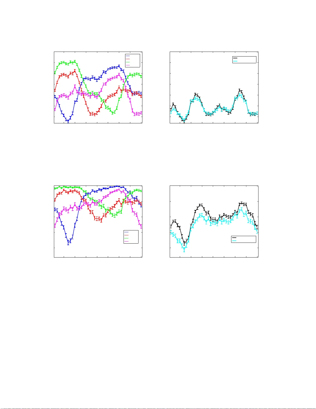
Multi-mo del Cross P ollination i n Time Hailiang Du 1 , 2 Leonard A. Smith 1 , 2 , 3 1 Cen ter for Robust Decis ion Making on Climate and Energy P olicy , Univ ersit y of Chicago, Chicago, IL, US 2 Cen tre f or the Analysis of Time Series, London Sc ho ol of Economics, London W C2A 2AE. UK 3 P em brok e College, Oxfor d, UK June 24, 2021 Abstract Predictive skill of complex mo dels is often not uniform in mo del-sta te space; in weather forecasting mo dels, for example, t he skill of the model can be grea ter in p opulated regio ns of int erest than in “r emote” regio ns of the glob e. Given a collectio n of mo dels, a multi-model forecast system using the cr oss pollina tion in time approa ch can b e gene r alised to take adv an- tage of instanc e s where some mo dels pro duce systematically more accur ate for ecast of some comp onents of the model- state. This g e neralisation is stated a nd then successfully demon- strated in a mo derate ( ∼ 40) dimensional nonlinea r dynamical system suggested b y L o renz. In this demonstr ation four imp erfect mo dels , each with similar global forecast s k ill, ar e used. F uture a pplications in weather foreca sting a nd in economic foreca sting a re dis cussed. The demonstration establishes that cro s s p ollinating forecas t tra jector ies to enrich the co llection of simulations upon which the forec a st is built can yie ld a new foreca st system with significantly more skills than the origina l multi-model foreca st s y stem. Keywor ds : multi-model ensemble; data assimilation; cross p ollination; structural mo del erro r. 1 In tro duction Nonlinear dynamical s ystems are frequen tly used to mo del physic al pro cesses such as fluid dynam- ics and weather. Uncertain t y in the obser v ations mak es iden tification of the exact state imp ossible 1 for a c haotic nonlinear system, wh ic h calls for f orecast based on an ensem ble of initial conditions to reflect the inescapable uncertain t y in the observ ations by captur ing the sensitivity of eac h par- ticular f orecast. In general, when forecasting real systems, f or example the Earth’s atmosphere as in w eather foreca sting, there is no reason to b eliev e that a p erf ect mo del exists. Generally the mo del class fr om whic h th e particular mo del equations are dra wn do es n ot cont ain a pro cess that is able to generate tr a jectories consisten t with the data. In order to tak e into accoun t b oth the stru ctural mo del error and uncertain ties in initial cond itions, the multimodel and ensem ble tec hniques can b e com bined to a new approac h, known as the m ulti-mo del ensemble concept (see [11, 16] ). In recen t ye ars, m ulti-mod el ensem bles ha v e b ecome p opular to ols to inv estig ate and accoun t for shortcomings due to stru ctural mo del error in we ather and climate sim ulation-based predictions on time scales from d a ys to seasons and cen turies ([14, 16, 26, 27]). While there h a v e b een some results suggesting that the multi -mo del ensemble forecasts outp erf orm the sin gle m o del forecasts in an RMS sense, for example [14, 27], Sm ith , et al. [22] challenge d th e claim that the m ulti-mo del ensemble provides a “b etter” prob ab ilistic forecast than the b est single mo d el. The current multi-mod el ensem ble forecasts are based on com bining single mod el ensemble forecasts only by means of statistically pro cessing m o del simulati ons to form the forecasts. T o th e exten t that eac h mo d el is dev elop ed ind ep endently , ev ery s ingle mo del is likely to conta in differen t lo cal (regional, for example) dy n amical in formation f r om that of other mo del; such information is not exp ected to b e explored by statistica l pro cessing. Using statistical pr o cessing, suc h information is only carried by the simulatio ns u nder a sin gle mo d el ensemble: n o adv an tage is take n to influence sim ulations und er the other mo dels. This pap er presents a n o v el metho d ology , named Multi- mo del C ross Polli nation in Time, for multi-model ensem ble sc heme with the aim of int egrating the dyn amical information from eac h ind ividual mo del op erationally in time instead of statistical pro cessing. The prop osed approac h generates mo del s tates in time via app lying data assimila- tion scheme(s) ov er the m ulti-mo del forecasts. Illustrated h ere using th e mo derate-order Lorenz mo del [15], th e prop osed approac h is demonstrated to allo w significant improv emen t up on the traditional statistica l pro cessing and b est single mo del ensem ble. It is su ggested th is illus tration could f orm the basis for m ore general results which in turn could p oten tially b e deplo y ed in op - erational forecasting. In we ather forecasting, th ere is a tendency to fo cus on mo del p erformance lo cally , North America for National Centers for Environmen tal Prediction (NCEP), Europ e f or Europ ean Centre for Medium-Range W eather F orecasts (ECMWF) and Asia for J apan Meteoro- 2 logica l Agency (JMA). The multi- mo del ensem ble forecast p roblem of interest is defin ed and traditional statistical pro cessing app roac hes are review ed in S ection 2. A full review of simple Multi-mo d el Cr oss P ollination in Time (CPT I) ap p roac h is presente d in Section 3. An adv anced Multi-mo del Cross P ollination in Tim e (CPT I I) app roac h is pr esen ted in Section 4. The exp erimen t based on Lorenz 96 system-mo dels p air is designed as wel l as the results are p r esen ted in Section 5. S ection 6 p r o vides discus s ion for wider app lications and conclusions. 2 Problem d escription Outside those pr oblems defined with in pur e mathematics, there is arguably n o p erfect m o del for p roblems includ ing a physica l dynamical s ystem [13, 23] ev olving smo othly in time. One h yp otheses a n on lin ear system with state space R ˜ m , the ev ol ution operator of the sy s tem is ˜ F (i.e. ˜ x ( t + 1) = ˜ F ( ˜ x ( t )) where ˜ x ( t ) ∈ R ˜ m is th e state of the system). ˜ F , ˜ x , and ˜ m are u n kno wn. It is often useful to sp eak as if su c h a system existed, regardless of wh ether or not one actually do es exist. An observ at ion of the sys tem state at time t is d efined by s ( t ) = ˜ h ( ˜ x ( t )) + η ( t ) where s ( t ) ∈ O , ˜ h is the observ ation op erator that pr o jects the system state on to observ ation space and η ( t ) r epresen ts the observ ati onal noise. What is in hand are M mo dels eac h of whic h appro ximates the system, with the form x ( t + 1; i ) = F i ( x ( t ; i )) , i = 1 , . . . , M , wher e x ( t ; i ) ∈ R m ( i ) , R m ( i ) is the mo del-state sp ace corresp onding to the i th mo del F i . In practice, m o del-state space us u ally differs from observ at ion space, and it is likely that differen t mo d els define different mo del-state space. The mo del states can b e pro jected into th e observ atio n space via an observ ation op erator h i ( · ), (different mo del m ay also ha v e different op erator). The simplest r eactio n to ha v e M mod els, eac h of wh ich pro vides N-mem b er ensemble forecast, migh t b e to identify the b est, discard others. If the mo dels are of comparable qualit y 1 , then it is like ly that d ifferen t mo dels will tend to do b etter in differen t regions of state s p ace (wea ther mo dels for example, on d ifferen t geographical lo cations or d ifferen t synoptic conditions), d ue to v a riations in the particular pr o cesses that are imp ortan t lo cally . 2 1 or even in t he case some mo dels are inferior on a verage but comp eting on o ccasion. 2 In practice, there is rarely enough data to identify which one will b e th e b est on a give n d ata [12], and a reasonable alternative is to compute M , N-mem b er ensembles, one ensem ble under each m o del and treat eac h ensem ble equally . 3 Consider eac h mo del pr o ducing an N-mem b er ens em ble forecasts b y iterating an N-mem b er initial condition ensem ble f orward. I n practice, such multi-model forecast system is verified u sing the future observ ations. The goal here in this pap er is to in tro duce new multi-model ensem ble forecast s ystem (in time) to improv e 3 forecast of the fu ture states. The Mo del Outpu t Statist ics (MOS) has a long and successful history of statistically pr o cessing single mo d el ensem ble forecasts (see [28, 29] and r eferen ces therein). F or m ulti-mo del ensem ble, statistica l approac hes ha v e b een pr op osed to combine ensembles of individual mo d el run s t o pro du ce a single probabilistic m ulti-mo del forecast distribu tion, mostly based on weigh ting th e mo dels according to some measure of p ast p erformance, for example [5, 9, 18]. Th e output of these statistic al pro cessing approac h es is a fu nction of eac h individ ual f orecast ensem b le. On ly the single mo del ens em ble forecast are conducted in time and carries some inf ormation of the mo del dynamics. Despite the multi-model en sem ble theme is designed to accoun t for mo d el inadequacy as d ifferen t mo d els h a v e different mo del stru cture, statistical ly pro cessing the mo d els outp ut can hardly exp lore the lo cal dynamical inform ation of eac h ind ividual mo d el. The extension of CPT approac hes pr esen ted in this pap er in tegrate the d ynamical information from eac h individual mo del in time and pro duce, truly new, multi-model tra jectories w hic h significan tly increases the information in the ens emble of sim ulations b ey ond that a v ailable to the original multi-model ensem ble forecast. Th is addition is gained by allo wing communicatio n b et w een different m o dels regarding tra jectories in the fu ture. 3 Multi-mo del Cross P ollination in Time I When the differen t mo dels hav e indep enden t structur al sh ortcomings, then cross-p ollinating tra- jectories b et ween mo dels to obtain truly m ulti-mo del tra jectories can allo w the ensem ble of tra- jectories to explore imp ortant regions of state sp ace the individu al mo dels j ust can’t reac h . Smith [21] in tro d uced the C ross P ollination in Time (hereafter CPT I) approac h exploiting the assumption that all the mod els sh are th e same mo del-state space 4 . Let ∆ t b e th e observ ation time where ev ery ∆ t time step an observ ation is recorded. F or simp licit y , at ev ery obs er v ation time all 3 The improveme nt is quantified by t h e information in p robabilistic forecasts reflected in − log 2 ( p ( Y )) (see [8] and Section 5). 4 or t h ere are known one-to-one maps whic h link t h eir in d ividual state space, given all the mo dels are iterated discretely . 4 the mo d els provide their mo d el outputs 5 . Let τ b e the cross p ollination time that ev ery τ a cross p ollination is take n place. Giv en M N-mem b er ensem bles of tra jectories made un der eac h m o del, firstly consider th e ensembles of states at t = τ as one large ensemble of N × M states in a mo del- state space. Secondly using some prun ing sc heme to red uce th is large ensemble to N-mem b er states in ord er to mainta in a manageable ensemble size. While the optimal pr uning sc heme is still an ob ject of researc h, th e simple approac h [21] of id en tifying nearest pair of states, an d then deleting the one mem b er from this p air of t w o s tates with the smallest second nearest neighbor distance, h as b een foun d to more effectiv e than ran d om selection in some simple examples. 6 In this pap er, a pru n ing sc h eme b ased on the lo cal forecast p erformance (see Section 5) is adopted to ser ve the pu rp ose of demonstrating the u se of pr op osed CPT I I approac h. Third ly use these N states as initial conditions and propagate them forw ard u nder eac h of the M mo d els to p ro duce M N-member ensembles of tra jectory segmen ts until the next cross p ollination time 2 τ . Rep eat these three steps unti l the forecast time of interest is reac hed, and then interpret the ensem ble [4]. Inasm uch as the CPT I ensemble scheme con tains implicitly all tra j ectories of eac h of its constituen t mo dels, the dynamical information of eac h ind ividual mo del is explored and integ rated. In practice, how ev er, the assumptions of this approac h are less lik ely to hold: differen t mo dels usually define differen t mo del-state space, and the one-to-one maps, w hic h link d ifferen t mo del- state space, ma y not exist for example in wea ther forecasting. More relev an t for the w ork b elo w, ho w ev er, is that CPT I traditionally considers the en tire mo d el state, without r egarding f or the fact that some mo d els migh t forecast some comp onents with greater skill. E ac h tra jectory segmen t un d er CPT I is a tra jectory of one of the M mo dels, the cross p ollination is of tr a jectory segmen ts; CPT I I aims to u se the inf ormation in these mo d el dynamics more effectiv ely . An other shortcoming of CP T I is that for eac h mo del the in itial conditions p ro duced by other mo dels are unlik ely to b e consisten t with that mo d el’s dynamics or b e efficien t and qualit y samp les of in itial conditions f or that mo del as iterating those initial conditions u nder the mo del for a short p erio d lik e τ ma y lead them to the mo del attractor. The CPT I I approac h introdu ced in the n ext section frees one from the assump tions and o vercomes su c h shortcomings. 5 Note it is often the case that the mo del iteration(simulatio n) step is muc h smaller than th e observ ation time, different models may ha ve different iteratio n step and pro d uce output s with different time frequ ency . 6 Note th at the aim prun ing is qu ite different than th at of resampling from an estimated PDF [2]. 5 4 Multi-mo del Cross P ollination in Time I I The Mu lti-mo d el Cross Po llination in Tim e (CPT I I) approac h pr esen ted here n ot only frees one from the assumption that all mo dels share the same mo del-state space bu t also extracts and in tegrates th e d ynamical inform ation from eac h mo del via exploring th e sequence space. The CP T I I approac h consists of three steps: (i) Com bine Multi-mo del outp uts in the observ ation sp ace to create an ensemble of orbits, eac h orbit consist of a sequ en ce of s tates in the observ ation space. F or eac h individu al mo del, the forecast ensemble is obtai ned via iterating an initial condition ensem ble forward un til the firs t CPT time τ , whic h pro d uces an ensem b le of mo d el tra jectory segmen ts, from time t 0 to t 0 + τ . Although d ifferen t mo dels ma y defin e different mod el-state space, every mo d el state can b e p r o jected on to observ ation sp ace u sing th e corr esp onding observ ation op er ator. A mo del tra jectory segmen t of the i th mo del, p ro jected onto obser v a- tion space, b ecomes an orbit, X ( i ) ≡ { h i (( x ( t 0 ; i )) , h i (( x ( t 0 + ∆ t ; i )) , . . . , h i (( x ( t 0 + τ ; i )) } , where t 0 is the initial time and x ( t + ∆ t ; i ) = F ∆ t i ( x ( t ; i )). F or M mo dels an d eac h pro d uces N-mem b er ensemble, it f orms one large ensem ble of M × N orbits X ( i, j ) , i = 1 , . . . , M and j = 1 , . . . , N in the observ ation space. Th ere are v arious statistical pro cessing approac hes to com b ine the multi-model ens emble of sequence states in the observ ation space, for example traditional MOS ap p roac h . And in order to main tain a manageable ensem ble size, one m a y prun e this large ensem ble b ac k into N sequences of states using some pr uning sc heme (the prun in g s cheme used in th is pap er is describ ed in th e follo wing section), that is: { X (1 , 1) , . . . , X (1 , N ) } . . . { X ( M , 1) , . . . , X ( M , N ) }            → { Y (1) , . . . , Y ( N ) } (1) Y is the co mbined outpu t of ensem ble sequence states in the observ ation sp ace, Y ( j ) ≡ { y ( t 0 ; j ) , y ( t 0 + ∆ t ; j ) , . . . , y ( t 0 + τ ; j ) } wh ere y ( t ; j ) ∈ O . (ii) Data assimilation of lo cally preferred en sem ble signals Giv en N sequences of states in the observ ation space, { Y (1),. . . , Y (N) } , eac h individ ual mo del can apply a data assimilation sc heme to eac h sequence of state to obtain a sequence 6 of mod el s tates in its mo del-state space, this corresp onds to treat a sequence of states in the obs erv ation sp ace as a sequence of observ ations: { Y (1) , . . . , Y ( N ) } →            { Z (1 , 1) , . . . , Z (1 , N ) } . . . { Z ( M , 1) , . . . , Z ( M , N ) } (2) Z ( i, j ) is the j th sequence of model states in the i th mo del state space, Z ( i, j ) ≡ { z ( t 0 ; i ; j ) , z ( t 0 + ∆ t ; i ; j ) , . . . , z ( t 0 + τ ; i ; j ) } where z ( t ; i ; j ) ∈ R m ( i ) . It is not necessary for eac h mo del to apply the same d ata assimilation sc heme (in practice, it is lik ely that eac h mo del has its o wn data assimilation sc heme), using existing data as- similation schemes w ould clearly av oid extra cost of imp lemen ting the CPT I I appr oac h. It is, how ev er, n oted that applying d ata assimilation h ere is cru cial in order to extract d ynam- ical information from the m o del. It is d esirable to use nonlinear data assimilation scheme whic h accoun ts for structural mo d el err or, for example Pseud o-orbit Data Assimilation (see Du and Smith [6, 7]), a b rief description is giv en in the App end ix A. As the mo d el is not p erfect, the d ata assimilation sc heme u sed h er e is n ot aiming to obtain mo d el tra jectories, but p s eudo-orbits [7]. P r o jecting the end comp onent of the m o del pseud o-orbits, obtained from th e data assimilation, int o the obs er v ation sp ace would provi de N × M forecast states at t = t 0 + τ . (iii) Iterate new mo del states (from ii) forward Consider th e end comp onen t of Z ( i, j ), z ( t 0 + τ ; i ; j ), as initial condition for the i th mo del and j th mem b er and ite rate forward using the i th mo del un til th e next cross p ollination time t 0 + 2 τ , w hic h pro duces an ensemble of mo d el tra jectory s egments, from time t 0 + τ to t 0 + 2 τ . Rep eat (i),(ii) and (iii) to pr o vid e f orecast states at t = t 0 + 2 τ and s o on to pro vide forecasts at t = t 0 + kτ , k = 3 , 4 , ... . Cross Poll ination in Time [21] differs fu ndament ally f rom other “forecast assimilation” tec h- niques. Stephens on et al. [25] for example introdu ced a no vel approac h to forecast assimilati on whic h generalizes earlier calibration metho ds includ ing mod el output statistics (see [30]). This approac h pro vides a m ap from the space of mo d el s imulations to the space of obs erv ations. In 7 general an y map from the model-state space to the target observ able s pace whic h u ses (only) information a v ailable at the time the forecast simulati ons were launc h is admissible. Bro c k er and Smith [4] d iscuss other appr oac hes to ensem ble in terp retations. None of these pap ers, ho we v er, enable th e f eedb ac k of forecast -simula tion information in to the dyn amics of the forecast itself. CPT I I do es precisely th is. 5 Exp erimen ts based on Lorenz96 A sys tem of nonlinear ord inary differential equations (Lorenz96 System) was introdu ced by Lorenz [15]. F or the system contai ning n v ariables x 1 , ..., x n with cyclic b oundary conditions (where x n +1 = x 1 ), the equations are dx i dt = − x i − 2 x i − 1 + x i − 1 x i +1 − x i + F, (3) The system is supp osed to represent a one-dimensional atmosphere; the n v ariables x 1 , ..., x n are to b e id en tified with the v alues of some uns p ecified scalar atmosph eric qu an tit y at n equally spaced p oints ab ou t a latitude circle wh ic h is called grid p oin ts, even though the “grid” is one- dimensional. [15] F is a p ositiv e constant, it is also found [15] th at as long as n > 12, c haos is found wh en F > 5. The true system (hereafter, system) used in th e follo wing exp eriments, con tains 40 v ariables, n = 40, and th e v alues of the parameter F v aries with lo cations, i.e. F = 8 for i = 1 , . . . , 10; F = 12 for i = 11 , . . . , 20; F = 14 for i = 21 , . . . , 30; F = 10 f or i = 31 , . . . , 40. F our mo d els eac h defined using the same dyn amical equation as the system bu t with fixed v alue of parameter F , that is: m o del I, F = 8 for all i ; mo del I I, F = 12; mo del I I I, F = 14 and m o del IV, F = 10. Both th e system and the mo del are defined using a s tandard fourth -order Runge-Kutta n u - merical simula tion. The simulatio n time step is 0 . 01 time un it and the mo del time s tep ∆ t is 0 . 05, that is eac h m o del time step is cond ucted b y 5 steps of th e fourth-order Runge-Kutta in tegra- tor. Ob serv ations s ( t ) ∈ R 40 are generated by th e system plu s I ID Gaussian noise, N (0 , σ 2 N ois e ), σ N ois e = 0 . 2, at ev ery system time step (0 . 05 time unit). 7 The cross p ollinatio n time τ = 0 . 4 indicates 2 da ys 8 . 7 In this setting, the mo del state space, system state space and the observ ation space are identical, although the prop osed CPT I I is not constrained to op erate in this ideal setting. 8 Assuming 1 time unit is equal to 5 days, th e doubling time of the Lorenz96 system roughly matches the 8 F or a forecast initial time t 0 , a simple inv erse noise metho d (adding dra ws from the inv erse of the observ ational noise to the ob s erv ation) is adopted to generate a 9-mem b er initial condition ensem ble for all th e mo dels, IC ( t 0 ) ≡ { x ( t 0 , j ) ∈ R 40 , j = 1 , ..., 9 } . Iterate the initial condition ensem ble forw ard und er eac h of the four mo dels until time t 0 + τ . F or eac h mo d el this gives an ensem ble of mo del tra jectories, for example for mo del I: { X ( I , 1) , . . . , X ( I , 9) } where X ( I , j ) ≡ { x ( t 0 ; I ; j ) , x ( t 0 + ∆ t ; I ; j ) , . . . , x ( t 0 + τ ; I ; j ) } , x ( t + ∆ t ; I ; j ) = F ∆ t I ( x ( t ; I ; j )) and x ( t ; I ; j ) ≡ { x 1 ( t ; I , j ) , x 2 ( t ; I , j ) , . . . , x 40 ( t ; I , j ) } ∈ R 40 . F or eac h mo d el, a large set of f orecasts is collecte d b y rep eating the ab ov e exp erimen ts for 4096 different initial states. Consider half of the set as training set to fit parameter v alues and the other half as test set for ev aluation. T o assess eac h mo del’s forecasts at v arious lead time, the forecast ensem ble is translated into predictiv e distribution fu n ction b y kernel dr essing and blending w ith climatologica l d istribution (for a full descrip tion see [4], and App end ix B). The forecast p erformance is ev aluated with IJ Goo d s logarithmic score (Ignorance score; [8, 19]). The Ignorance score is the only prop er lo cal score for con tin uous v ariables [1, 3, 17]. Although there are other n onlo cal pr op er scores, the auth ors pr efer usin g ignorance as in addition it has a clear interpretatio n in terms of information theory wh ic h can b e easily comm unicated in terms of effectiv e in terest returns [10]. 9 Ignorance is defi n ed by: S ( p ( y ) , Y ) = − log 2 ( p ( Y )) , (4) where Y is the outcome and p ( Y ) is th e probabilit y of the outcome Y . In practice, giv en K forecast-outco me pairs { ( p i , Y i ) | i = 1 , . . . , K } , th e empirical a ve rage Ignorance score of a forecast system is then S E ( p ( y ) , Y ) = 1 K K X i =1 − log 2 ( p i ( Y i )) , (5) Figure 1a, 2a and 3a shows th e empir ical Ignorance relativ e to climatology for eac h mo del at differen t lo cation (dimension) at lead time τ , 2 τ and 3 τ . The emp irical Ignorance is calculate d based on 2048 forecast outcome pairs and the climatolo gical d istribution is estimated u sing 2048 historical observ ations. chara cteristic time-scale of dissipation in th e atmosphere (see Lorenz [15]). 9 There are no comp elling ex amples in fa vor of the general use of nonlo cal scores and some nonlo cal scores h a ve b een shown to pro du ce counter intuitiv e ev aluations [24]. 9 5 10 15 20 25 30 35 40 −3 −2.5 −2 −1.5 −1 −0.5 0 Location Ignorance relative to climatology Forecast at lead time τ (day 2) Model I Model II Model III Model IV (a) 5 10 15 20 25 30 35 40 −3 −2.5 −2 −1.5 −1 −0.5 0 Location Ignorance relative to climatology Forecast at lead time τ (day 2) Pure multi−model CPT II (b) Figure 1: I gn oran ce s core of forecasts as a fun ction of lo cation (d imension) at lead time τ = 0 . 4 time un it, a) forecasts from eac h individual mo del, b) pur e m u lti-mo d el forecast (Blac k) and CPT I I forecast (Cya n). 5 10 15 20 25 30 35 40 −2 −1.5 −1 −0.5 0 Location Ignorance relative to climatology Forecast at lead time 2 τ (day 4) Model I Model II Model III Model IV (a) 5 10 15 20 25 30 35 40 −2 −1.5 −1 −0.5 0 Location Ignorance relative to climatology Forecast at lead time 2 τ (day 4) Pure multi−model CPT II (b) Figure 2: Ignorance score of forecasts as a function of lo cation (dimension) at lead time 2 τ = 0 . 8 time un it, a) forecasts from eac h individual mo del, b) pur e m u lti-mo d el forecast (Blac k) and CPT I I forecast (Cya n). A simple pru ning algorithm is adopted to maint ain a m anageable ens em ble size, wh ic h pru nes four model (9-mem b er) ensem b le f orecast tra jectories into 9 sequences of states (see Equation (1)): Defin e the pr uned ensemble orbits to b e { Y (1) , . . . , Y (9) } where Y ( j ) ≡ { y ( t 0 ; j ) , y ( t 0 + ∆ t ; j ) , . . . , y ( t 0 + τ ; j ) } and y ( t ; j ) ≡ { y 1 ( t ; j ) , y 2 ( t ; j ) , . . . , y 40 ( t ; j ) } ∈ R 40 . Assign the v alue of x i ( t, B , j ) to y i ( t ; j ), where B is historically the lo cal b est mo del among (I, I I, I I I, IV) th at pr o duce b est (Ignorance) forecasts at lead time τ for dimension lo cation i . 10 5 10 15 20 25 30 35 40 −1.2 −1 −0.8 −0.6 −0.4 −0.2 0 Location Ignorance relative to climatology Forecast at lead time 3 τ (day 6) Model I Model II Model III Model IV (a) 5 10 15 20 25 30 35 40 −1.2 −1 −0.8 −0.6 −0.4 −0.2 0 Location Ignorance relative to climatology Forecast at lead time 3 τ (day 6) Pure multi−model Pure multi−model (36m−Ens) CPT II (b) Figure 3: Ignorance score of forecasts as a function of lo cation (dimension) at lead time 3 τ = 1 . 2 time unit, a) forecasts fr om eac h individual mo d el, b) pure multi- mo del forecast (Blac k), pure m ulti-mo del forecast with 36-mem b er ensem b le fr om eac h model (Bro wn) and CPT I I f orecast (Cy an). T o demonstr ate the u se of CPT I I appr oac h, the outputs f rom pure mo del approac h are compared with the results f rom CPT I I approac h at lead time τ , 2 τ and 3 τ . Note th at b oth the outputs from pure mo del ru ns and those from CPT I I app r oac h at an y lead time t are m ulti- mo del ensem b le. The m ulti-mo del ensem ble is interpreted by com bining the f orecast d istributions, generated from ens embles of individu al m o del outp uts to p r o duce a single probabilistic m u lti- mo del forecast distribution for ev aluation. A linearly we ight ed approac h is adopted to com b in e the s in gle mo d el forecast distr ibution (for a f u ll description see [12], and App endix C). Figure 1b, 2b and 3b compares the probabilistic forecasts from the pure m ulti-mo del out- puts(Blac k) with those f r om CP T I I(Cy an) at lead time τ , 2 τ and 3 τ . A t lead time τ , the dynamical information from eac h individual are com b ined and embedd ed into the forecasts wh ic h are also the initial states of the forecasts for the next cross p ollination p erio d. Suc h additional information in the initial cond itions rev eals its v alue at th e n ext forecast p erio d, where significan t impro v ement in skill is sh own at lead time 2 τ and 3 τ . Note in figure 3b that the CPT I I forecast also signifi can tly ou tp erforms th e pu r e m ulti-mo del forecast (Bro wn ) based on f our times larger ensem ble size (eac h mo d el pro d uces 36-mem b er ensem ble forecast). In th is pap er, CPT I I exploits the sophisticated PDA data assimilation sc heme [6, 7] to allo w selectiv e inclus ion of lo cations (state s pace comp onents) in the forecast simulatio n of eac h mo d el. 11 Doing so allo ws CPT forecast sy s tem to general forecasts with supp ort b ey ond that of with simple mo del f orecast systems or traditional multi-model forecast systems. As demons tr ated ab ov e, it is p ossible th at this approac h increases forecast skill. 6 Conclusion Supp ose f or a moment one has tw o mo dels which simulate sup ply and demand, giv en the current supply and demand. Mo del A pro duces significan tly b etter forecasts of s upply , w hile Mo del B yields significan tly b etter forecasts of demand. The traditional m ulti-mo del approac h is to consider an en sem ble of simulatio n un d er mo del A and a s econd indep enden t ensemble of sim ulations u nder mo del B. The sp ecific mo del inadequacy in eac h mo del will r esult in a deca y in the relev ance of the probabilistic forecasts with lead time. Cross P ollination in Time I I aims to dela y this deca y , extending the lead-time of inf orm ativ e forecasts, by assimilating forecasts of the near-term future to generate an enhanced ensem ble of forecasts in the m edium range, and iterating the pro cess in to the long range. I n this simple case, taking the “sup p ly” forecast from mo del A and the “demand” foreca st from Mod el B would pr o duce a new initial condition to b e folded into the forecast ensem bles of eac h mo del at lead time one and propagated into the future, improving the abilit y to forecast. By con tract, th e state of a m o dern wea ther m o del consists of (more than) tens of millions of comp onent s, and no tw o op erational mo dels actually sh are the same mo d el-state space. CPT I I o vercomes this c hallenge b y using a d ata assimilation designed to start with a p seudo-orbit, and an initial ps eu do-orbit extracted from the initial simula tion tra jectory of eac h mo del. Th is approac h yields probabilistic forecasts more skillful than traditional approac hes, ev en when the ensem ble size of the traditional appr oac h is increased by a factor of four. As noted ab o ve, c hallenges remain in deploying and interpreting CPT I I forecast systems; this concrete example of success is in tend ed to motiv ate exploration of more realistic cases. APPENDIX 12 A Pseudo-orbit Data A ssimilation A brief descrip tion of the PDA approac h is giv en in the follo win g p aragraphs (for more details, see Du and S mith [6, 7]). Let the dimension of the mo d el-state space b e m and the n umb er of observ ation times in the assimilation window b e n (for exp er im ents presented in this pap er, n = τ ∆ t ). A pseudo- orbit , U ≡ { u − n +1 , ..., u − 1 , u 0 } , to is a p oin t in th e m × n dimensional sequence space for whic h u t +1 6 = F ( u t ) for any comp onent of U . Define the comp onent of the mismatch of a pseu d o-orbit U at time t to b e e t = | F ( u t ) − u t +1 | , t = − n + 1 , ..., − 1 and the mismatc h cost fun ction to b e C ( U ) = X e 2 t (6) The P seudo-orbit Data Assimilation minimizes the mismatc h cost function for U in the m × n dimensional sequen ce sp ace via gradient descen t (GD) minimization algorithm. F or CPT I I, such minimization is initialized with the com bined m o del output of sequence states in the observ ation space, Y(j) in Equation (1) and (2). An imp ortant adv an tage of PD A is that the minimization is done in the sequence sp ace: information fr om across the assimilation win do w is used simulta- neously . The ps eudo-orbit U is up dated on every iteration of the GD minimizatio n. Let the resu lt of the GD minimization b e α U where α indicates algorithmic time in GD. Due to the mo del imp erf ection, the minimization is applied with a stopping criteria in order to obtain more consisten t pseudo- orbits [7] as the mismatc hes r eflect the p oin t-wise mo del error, w hic h is kno wn to exist when the mo del is imp erfect. In the exp eriment s pr esen ted in this pap er the s topp ing criteria targeted forecast p erformance at lead time τ , 2 τ and 3 τ . B Ensem ble In terpretation An ensemble of sim ulations is transformed into a pr obabilistic distribution f u nction b y a com bi- nation of kernel dr essing and blending with climato logical distribution (see [4]). An N -member ensem ble at time t is give n as X t = [ x 1 t , ..., x N t ], where x i t is the i th ensemble mem b er. F or sim- plicit y , all en sem ble memb ers un der a mo d el are treated as exchangea ble. Kernel d r essing defines the m o del-based comp onen t of the d ensit y as: p ( y : X, σ ) = 1 N σ N X i K  y − ( x i − µ ) σ  , (7) 13 where y is a r an d om v ariable corresp ond ing to the density function p and K is the k ernel, tak en here to b e K ( ζ ) = 1 √ 2 π exp ( − 1 2 ζ 2 ) . (8) Th us eac h ensem ble mem b er con tributes a Gaussian kernel cen tred at x i − µ . Here µ is an offset, whic h accoun ts for any systematic “bias”. F or a Gaussian k ern el, the k ernel width σ is simply the s tand ard deviation. F or an y finite ensem ble, there remains the chance of ∼ 2 N that the outcome lies outside the range of the ensem ble ev en w hen the outcome is s elected from th e same distribution as the ensem ble itself. Giv en the nonlinearity of the mo del, s uc h outcomes can b e v ery far outside the range of the ensem ble mem b ers. In ad d ition to N b eing fin ite, in practice , of course, the sim ulations are not drawn from the same distribu tion as the outcome as the ensemble simulat ion system is not p erfect. T o improv e the skill of the probab ilistic forecasts, the kernel dressed ensem ble m a y b e blended with an estimate of the climatological distribution of the sys tem (see [4] for more details, [20] for an alternativ e ke rnels and [17 ] for a Ba y esian approac h ). The b lended forecast d istribution is then written as p ( · ) = αp m ( · ) + (1 − α ) p c ( · ) , (9) where p m is the density function generated b y dressin g the mo d el ensemble and p c is the estimate of climatolo gical den s it y . The b lending p arameter α determines h o w m uch weig ht is p laced in the mo del. Sp ecifying the thr ee v alues (the offset µ , the k ernel w id th σ , and the blend ed parameter α ) defines the forecast distribution. These p arameters are fitted simultaneously by optimising the empirical Ignorance score in the training set. C W eigh ting Multi-mo del Ensem ble There are many wa ys in whic h forecast distribu tions, generated from ensem bles of individu al mo del ru ns can b e com bined to p ro duce a single pr ob ab ilistic m ulti-mo del forecast d istribution. One app roac h ma y b e to assign equal wei ght to eac h mo del and simp ly sum the d istributions generated from eac h mo del to obtain a single p robabilistic distribu tion (see [9]). In general, differen t forecast mo d els do not provide equal amounts of information, on e m a y w ant to weig ht 14 the mo dels according to some measure of past p erform an ce, see for example [5, 18]. The com b in ed m ulti-mo del forecast is the we igh ted linear sum of the constituen t distribu tions, p mm = X i ω i p i , (10) where the p i is the forecast distribu tion f rom mo del i and ω i its w eigh t, with P i ω i = 1. Th e w eigh ting paramete rs m ay b e c hosen by minimizing the Ignorance score for exa mple, although fitting ω i in this wa y can b e costly and is t ypically complicated by different mo dels sharing information. And , of course, the weigh ts of ind ividual mo d els are exp ected to v ary as a fun ction of lead time. T o a vo id ill fitting mo del w eigh ts a simple iterativ e metho d to com bine mo d els is adopted in- stead of fitting all the w eigh ts simultaneously . F or eac h lead time, the b est (in terms of Ignorance) mo del is fi r st com b ined w ith the second b est mo del to f orm a combined forecast distr ibution (b y assign w eights to b oth mo dels). Th e com bined forecast distribution is then com bined with the third b est mo d el to up d ate the combined forecast distribu tion. Rep eat this pro cess until the w orst mo del is included. Ac k no wledgmen t This researc h wa s sup p orted by the LSE’s Grantham Research In stitute on Climate Change and the Envi ronment and the ESRC Cen tre for Climate C h ange Economics and Poli cy , f u nded b y the Economic and So cial Researc h Council and Munich Re; it wa s also fu nded as p art of the EPSRC- funded Blue Green Cities (EP/K013661 /1). Ad ditional sup p ort for H.D. w as also pr o vid ed by the National Science F ound ation Aw ard No. 09 51576 “DMUU: Cen ter for Robust Decision Making on Climate and E n ergy Polic y (RDCEP)”. L.A. S. gratefully ac kno wledges the cont inuing supp ort of Pem br ok e College, Oxford . References [1] J. M. Bernardo. Exp ected in formation as exp ected u tilit y . Ann. S tat., 7:686-690, 1979. [2] C. H. Bishop, B. J. Etherton, and S. J. Ma jum dar. Adaptiv e Sampling with the Ensemble T ransform Kalman Filter. Part I: Theoretical Asp ects. Mon. W ea. Rev., 129(3) :420-436 , 2001. 15 [3] J. Bro ck er and L.A. S mith. S coring probabilistic f orecasts: On 356 the imp ortance of b eing prop er. W ea. F orecasting, 22:382 -388, 2007. [4] J. Bro ck er and L.A. S m ith. F rom ensem b le forecasts to predictiv e distribution fu nctions. T ellus, 60:663 678, 2008. [5] F. J. Doblas-Rey es, R. Hagedorn, and T. N. P almer. T he rationale b ehind the success of m ulti-mo del ensembles in seasonal forecasting. part ii: Calibration an d combinatio n. T ellus A, 57:234, 2005. [6] H. Du and L.A. Smith. Ps eu do-orbit data assimilation part I: th e p erfect m o del scenario. Journal of the A tmospheric Sciences, 71(2):4 69-482, 2014. [7] H. Du and L.A. Smith. Pseudo-orbit data assimilation part I I: assimilation with imp erfect mo dels. Journal of the A tmospheric Sciences, 71(2):483-4 95, 201 4. [8] I. J. Go o d. Rational decisions. Jour nal of the Roy al S tatistica l So ciet y , XIV(1), 1952. [9] R. Hage dorn , F. J. Doblas-Rey es, and T. N. Palmer. T h e rationale b ehind the success of m ulti-mo del ensem bles in s easonal forecasting. part i: Ba sic concept. T ellus A, 57:219, 2005. [10] R. Hagedorn and L. A. Smith. Communicat ing the v alue of probabilistic forecasts with w eather roulette. Meteor. Appl., 16:14315 5, 2009. [11] M. S. J. Harr ison, T. N. Pa lmer, D. S. Ric hardson, R. Buizza, and T. P etroliagis. Joint en - sem bles f rom the ukmo and ecm w f mo dels. In EC MWF Seminar Pro cedin gs: Predictabilit y , v olume 2, page 61120, EC MWF, Readin g, UK, 1995. [12] S. Higgins, H. Du, and L.A. Smith. On the design and u se of ensembles of multi-model sim ulations for forecasting. In preparation for Nonlinear Pro cesses in Geoph ysics, 2016. [13] K. Ju d d and L.A. Sm ith . Ind istinguishable states ii: The imp erfect mo del scenario. Physica D, 196:224, 2004. [14] B. P . K irtman, D. Min, J. M. Infanti, J. L. Kinte r, D. A. Pa olino, Q. Zhang, H. v an den Do ol, S. Saha, M. P . Mendez, E. Bec k er, P . P eng, P . T ripp, J. Huang, D. G. DeWitt, M. K. Tipp ett, A. G. Barn ston, S. L i, A. Rosati, S. D. Sch ub ert, M. Rienec ke r, M. S uarez, 16 Z. E. Li, J. Marshak, Y. Lim, J. T rib bia, K. Pegio n, W. J. Merryfield, B. Denis, and E. F. W o o d. The North American Multimo d el Ensemble: Phase-1 Seasonal-to-In terannual Prediction; Ph ase-2 to ward Dev eloping Intraseasonal Prediction. Bull. Amer. Meteor. S o c., 95(4): 585-601, 2013. [15] E. N. Lorenz. Predictabilit y - a p roblem p artly solv ed. Cambridge Un iv ersit y Press, 1996. [16] T. N. P almer, F. J. Doblas-Rey es, R. Hagedorn, A. Alessandr i, S. Gualdi, U. And er s en, H. F eddersen, P . C an telaub e, J. M. T erres, M. Da ve y , R. Graham, P . Delecluse, A. Lazar, M. Deque, J. F. Guerem y , E. Dez, B. O rfila, M. Hoshen, A. P . Morse, N. K eenlysid e, M. Latif, E. Maisonna ve , P . Rog el, V. Marletto, and M. C. Thomson. Dev elopmen t of a europ ean m ultimo del ensem ble system for seasonal-to-in terann ual p rediction (demeter). Bull. Amer. Meteor. S o c., 85(6):85 3-872, 2004. [17] A. E. Raftery , T. Gneiting, F. Balab d aoui, and M. P olak owski. Using bay esian mo del a v er- aging to calibrate forecast ensembles. Mon. W ea. Rev., 133:11 55-1174 , 2005. [18] B. Ra jagopalan, U. Lall, and S. E. Zebiak. Categorical climate forecasts thr ough regularization and optimal com bination of m ultiple gcm ensem bles. Mon thly W eather Review,130: 1792-181 1, 2002. [19] M. S. Roulston and L. A. S mith. Ev aluating p robabilistic forecasts usin g inf orm ation theory . Mon. W ea. Rev., 130:1653- 1660, 2002. [20] M. S. Roulston and L. A. Smith. Com b ining dynamical and s tatistical ens embles. T ellus, 55:16- 30, 2003. [21] L. A. Smith. Disen tangling uncertain ty and err or: On the predictabilit y of nonlinear systems. In Alistair I . Mees, editor, Nonlinear Dynamics and S tatistics, c hapter 2, pages 31-64. Birkhauser Boston, 2000. [22] L. A. Smith, Hailia ng Du, Emma B. Suc kling, and F alk Niehrster. Probabilistic skill in ensem ble seasonal forecasts. Qu arterly Journal of the Ro yal Meteorological So ciet y , 141(6 89):1085 -1100, 2015. [23] L.A. Smith. What migh t w e lea rn from clima te forecasts? In Pr o c. National Acad. S ci., v olume 4, pages 2487-2 492, USA, 2002. 17 [24] L.A. Smith, E.B. Suc kling, E.L. Thompson, T. Ma ynard , and H. Du. T o w ards impr oving the f ramew ork for pr obabilistic forecast ev aluation. C limatic C h ange, 2015. [25] D.B. Stephenson , C. C o elho, F. Doblas-Rey es, and M. Alonso Balmaseda. F orecast as- similation: a u nified framework for the com bination of multimodel w eather and climate predictions. T ellus A, 57:253-2 64, 2005. [26] B. W ang, J. Lee, I. Kang, J . Sh ukla, C. K. P ark, A. Kumar, J. Sc hemm, S. Co c ke, J. S. Kug, J. J . Lu o, T . Z h ou, B. W ang, X. F u, W. T. Y un, O. Alv es, E. Jin, J. Kint er, B. Kirtman, T. Krishnamurti, N. Lau, W. Lau, P . Liu, P . Pegi on, T. Rosati, S . Sch ub ert, W. Stern, M. Suarez, and T. Y amagat a. Adv ance and prosp ectus of seasonal prediction: assessment of the APCC/CliP AS 14-mo del en s em ble retrosp ectiv e seasonal prediction (1980- 2004). Climate Dynamics, 33(1):9 3-117, 2009. [27] A. W eisheimer, F. J. Doblas-Re ye s, T. N. P almer, A. Alessandri, A. Arribas, M. Deque, N. Keenlysid e, M. MacV ean, A. Nav arra, and P . Rogel. ENS EMBLES: A new multi-model ensem ble for seasonal-to-ann ual predictions skill and pr ogress b ey on d DEMETE R in fore- casting tr opical Pa cific SS Ts. Geoph ysical Researc h Letters, 36(21 ), 2009. [28] D. S . Wilks. Comparison of en s em ble-MOS metho ds in the Lorenz96 setting. Meteorological Applications, 13:243 -256, 2006. [29] D. S. Wilks and T. M. Hamill. Comparison of Ens em ble-MOS Metho d s Using GFS Refore- casts. Mon. W ea. Rev., 135(6): 2379, 2007. [30] D.S. Wilks. S tatistical Metho ds in the A tmospheric S ciences. Academic Press, s econd edi- tion, 2005. 18