3D Visibility Representations of 1-planar Graphs

We prove that every 1-planar graph G has a z-parallel visibility representation, i.e., a 3D visibility representation in which the vertices are isothetic disjoint rectangles parallel to the xy-plane, and the edges are unobstructed z-parallel visibilities between pairs of rectangles. In addition, the constructed representation is such that there is a plane that intersects all the rectangles, and this intersection defines a bar 1-visibility representation of G.

💡 Research Summary

The paper investigates three‑dimensional visibility representations for the class of 1‑planar graphs, i.e., graphs that can be drawn in the plane so that each edge is crossed at most once. The authors introduce the notion of a z‑parallel visibility representation (ZPR): each vertex is mapped to an axis‑aligned rectangle lying in a plane parallel to the xy‑plane, and each edge is realized as an unobstructed visibility (a thin cylinder) parallel to the z‑axis that connects the two corresponding rectangles without intersecting any other rectangle. A ZPR is called k‑visible if there exists a plane orthogonal to the rectangles whose intersection with the ZPR yields a bar k‑visibility representation; the focus of this work is the case k = 1.

The main result, Theorem 1, states that every 1‑planar graph G with n vertices admits a 1‑visible ZPR of volume O(n³). Moreover, if a 1‑planar embedding of G is supplied (necessary because recognizing 1‑planarity is NP‑complete), the representation can be constructed in linear time O(n). The authors achieve this by building on the existing linear‑time algorithm of Brandenburg (2014) that produces a bar‑1‑visibility drawing of any 1‑planar graph.

The construction proceeds in three phases:

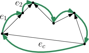
1. Bar‑1‑visibility drawing (γ₁).
   Starting from G, the algorithm first augments the graph to a 1‑plane multigraph G₀ in which every pair of crossing edges forms an empty kite (a K₄ with two crossing edges). Removing the crossing edges yields a planar multigraph P. By orienting P into a planar st‑multigraph Pᴼ (using a known orientation technique), the Tamassia‑Tollis algorithm is applied to obtain a bar visibility representation of Pᴼ. The crossing edges are then re‑inserted, extending some bars so that each newly introduced visibility traverses at most one bar. The resulting drawing γ₁ lies on an integer grid of size O(n²).

2. Initial 3D rectangles (γ₂).
   Each bar bᵥ of γ₁ is lifted to a rectangle Rᵥ that retains the same x‑interval and the same z‑coordinate as the bar, while initially setting its y‑extent to