Generating Multiple Diverse Hypotheses for Human 3D Pose Consistent with 2D Joint Detections

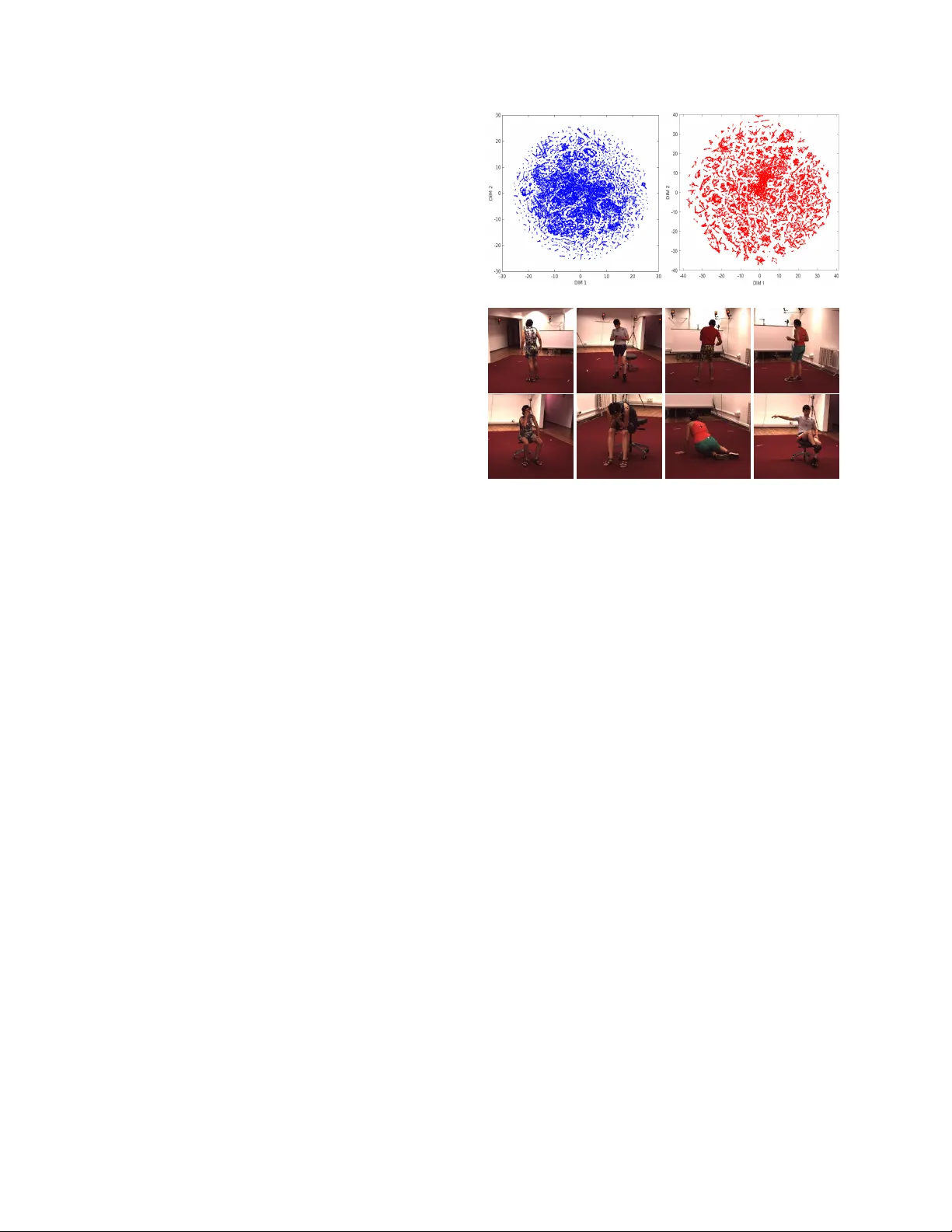
Generating Multiple Div erse Hypotheses f or Human 3D P ose Consistent with 2D Joint Detections Ehsan Jahangiri, Alan L. Y uille Johns Hopkins Uni versity , Baltimore, USA ejahang1@jhu.edu, alan.yuille@jhu.edu Abstract W e pr opose a method to generate multiple diverse and valid human pose hypotheses in 3D all consistent with the 2D detection of joints in a monocular RGB image. W e use a novel generative model uniform (unbiased) in the space of anatomically plausible 3D poses. Our model is com- positional (pr oduces a pose by combining parts) and since it is restricted only by anatomical constraints it can gen- eralize to every plausible human 3D pose. Removing the model bias intrinsically helps to gener ate mor e diverse 3D pose hypotheses. W e argue that generating multiple pose hypotheses is mor e r easonable than generating only a sin- gle 3D pose based on the 2D joint detection given the depth ambiguity and the uncertainty due to occlusion and imper- fect 2D joint detection. W e hope that the idea of generating multiple consistent pose hypotheses can give rise to a new line of futur e work that has not received much attention in the liter atur e . W e used the Human3.6M dataset for empiri- cal evaluation. 1. Introduction Estimating the 3D pose configurations of complex artic- ulated objects such as humans from monocular RGB im- ages is a challenging problem. There are multiple factors contributing to the dif ficulty of this critical problem in com- puter vision: (1) multiple 3D poses can have similar 2D pro- jections. This renders 3D human pose reconstruction from its projected 2D joints an ill-posed problem; (2) the human motion and pose space is highly nonlinear which makes pose modeling dif ficult; (3) detecting precise location of 2D joints is challenging due to the v ariation in pose and appear- ance, occlusion, and cluttered background. Also, minor er- rors in the detection of 2D joints can hav e a large effect on the reconstructed 3D pose. These factors fav or a 3D pose estimation system that takes into account the uncertainties and suggests multiple possible 3D poses constrained only by reliable evidence. Often in the image, there exist much Figure 1. The input monocular image is first passed through a CNN-based 2D joint detector which outputs a set of heatmaps for soft localization of 2D joints. The 2D detections are then passed to a 2D-to-3D pose estimator to obtain an estimate of the 3D torso and the projection matrix. Using the estimated 3D torso, the projection matrix, and the output of the 2D detector we generate multiple di verse 3D pose hypotheses consistent with the output of 2D joint detector . more detailed information about the 3D pose of a human than the 2D location of the joints (such as contextual infor- mation and dif ference in shading/texture due to depth dis- parity). Hence, most of the possible 3D poses consistent with the 2D joint locations can be rejected based on more detailed image information ( e.g . in an analysis-by-synthesis framew ork or by in vestig ating the image with some mid- lev el queries such as “Is the left hand in front of torso?”) or by physical laws ( e.g . gravity). W e can also imagine scenar - ios where the image does not contain enough information to rule out or fav or one 3D pose configuration over another especially in the presence of occlusion. In this paper, we focus on generating multiple plausible and div erse 3D pose hypotheses which while satisfying humans anatomical con- straints are still consistent with the output of the 2D joint 1 detector . Figure 1 illustrates an ov ervie w of our approach. The space of valid human poses is a non-con ve x com- plicated space constrained by the anatomical and anthro- pomorphic limits. A bone never bends beyond certain an- gles with respect to its parent bone in the kinematic chain and its normalized length, with respect to other bones, can- not be much shorter/longer than standard values. This inspired Akhter and Black [ 1 ] to build a motion capture dataset composed of 3D poses of fle xible subjects such as gymnasts and martial artists to study the joint angle limits. The statistics of 3D poses in this motion capture dataset is dif ferent from the previously existing motion cap- ture datasets such as CMU [ 11 ], Human 3.6M [ 15 ], and HumanEva [ 28 ], because of their intention to explore the joint angle limits rather than performing and recognizing typical human actions. Figure 2 shows the t-SNE visual- ization [ 36 ] of poses from A khter& B lack motion C apture D ataset ( ABCD ) versus H36M in two dimensions. One can see that the “ ABCD” dataset is more uniformly distrib uted compared to the H36M dataset. W e randomly selected 4 poses from the dense and surrounding sparse areas in the H36M t-SNE map and have sho wn the corresponding im- ages. One can see that all of the four samples selected from the dense areas correspond to standing poses whereas all of the four samples selected from sparse areas correspond to sitting poses. T raining and testing a 3D model on a similarly biased dataset with excessi ve repetition of some poses will re- sult in reduced performance on no vel or rarely seen poses. As a simple demonstration, we learned a GMM 3D pose model [ 29 ] from a uniformly sampled set of Human 3.6M poses (all 15 actions) and e valuated the likelihood of 3D poses per action under this model. The av erage likelihood per action (up to a scaling factor) w as: Directions 0.63, Dis- cussion 0.74, Eating 0.56 , Greeting 0.63 , Phoning 0.28 , Posing 0.38 , Purchases 0.55 , Sitting 0.07 , Sitting Down 0.07 , Smoking 0.47 , T aking Photo 0.23 , W aiting 0.33 , W alking 0.64 , W alking Dog 0.29 , and W alk T ogether 0.25. According to the GMM model, the “Discussion” poses are on average almost 10 times more likely than “Sitting” poses which is due to the dataset and consequently the model bias. The EM algorithm used to learn the GMM model attempts to maximize the likelihood of all samples which will lead to a biased model if the training dataset is biased. Ob viously , any solely data-driv en model learned from a biased dataset that does not cover the full range of motion of human body can suffer from lack of generalization to nov el or rarely seen yet anatomically plausible poses. W e propose a no vel generativ e model on human 3D poses uniform in the space of physically valid poses (sat- isfying the constraints from [ 1 ]). Since our model is con- strained only by the anatomical limits of human body it does not suffer from dataset bias which is intrinsically helpful to (a) (b) Figure 2. (a): The t-SNE visualization of poses from the H36M (fist from left) and ABCD (second from left). (b): The images corresponding to the random selection of poses from the dense (top row in right) and sparse (bottom row in right) area of the H36M t-SNE map confirm the dataset bias tow ard standing poses compared to sitting poses. div ersify pose hypotheses. Note that the pose-conditioned anatomical constraints calculated in [ 1 ] w as originally used in a constrained optimization frame work for single 3D pose estimation and turning those constraints into a generativ e model to produce uniform samples is not trivial. One of our main contributions is a pose-conditioned generati ve model which has not been done previously . W e generate multiple anatomically-valid and di verse pose hypotheses consistent with the 2D joint detections to in vestigate the importance of having multiple pose hypotheses under depth and missing- joints ( e.g . caused by occlusion) ambiguities. In the recent years, we have witnessed impressi ve progress in accurate 2D pose estimation of human in various pose and appear- ances which is made possible thanks to deep neural net- works and lots of annotated 2D images. W e take advantage of the recent advancement in human 2D pose estimation and seed our multi-hypotheses pose generator by an off- the-shelf 3D pose estimator . Namely , we use the “Stacked Hourglass” 2D joint detector [ 19 ] and the 2D-to-3D pose estimators of Akhter&Black [ 1 ] and Zhou et al. [ 42 ] to es- timate the 3D torso and projection matrix. Howe ver , note that to our generic approach does not rely on any specific 2D/3D pose estimator and can easily adopt various 2D/3D pose estimators. After briefly discussing some related works in subsec- tion 1.1 we propose our approach in section 2 . Our exper - imental results based on multiple 3D pose estimation base- lines is giv en in section 3 . W e conclude in section 4 . 2 1.1. Related W ork There are quite a few works in the human pose estima- tion literature that are directly or indirectly related to our work. Reviewing the entire literature is obviously be yond the scope of this paper . Sev eral areas of research are related to our work such as 2D joiont detection, 3D pose estimation, and generativ e 3D pose modeling. Due to the advancements made by deep neural networks, the most recent works on 2D joint detection are based on con volutional neural networks (CNN) [ 35 , 9 , 34 , 10 , 40 , 39 , 38 , 19 , 6 , 26 ] compared to the traditional hand-crafted feature based methods [ 27 , 41 , 12 ]. On the other hand, most of the 3D pose estimation meth- ods use sparse coding based on an overcomplete dictionary of basis poses to represent a 3D pose and fit the 3D pose projection to the 2D joint detections [ 24 , 37 , 1 , 42 , 43 ]. Some works [ 8 , 25 , 26 ] try to train a deep network to di- rectly predict 3D poses. Ho we ver , purely discriminativ e ap- proaches for 3D structure prediction (such as [ 8 ]) are usu- ally very sensiti ve to data manipulation. On the other hand, it has been shown that the deep networks are very effecti ve and more robust at detecting 2D templates (compared to 3D structures) such as human 2D body parts in images [ 19 ]. W e use conditional sampling from our generative model to generate multiple consistent pose hypotheses. A number of previous works [ 7 , 30 , 2 , 4 , 5 ] hav e used sampling for human pose estimation. Howe ver , the sampling performed by these works are for purposes dif ferent from our goal to generate multiple div erse and valid pose hypotheses. For example, Amin et al. [ 2 ] use a mixture of pictorial structures and perform inference in two stages where the first stage reduces the search space for the second inference stage by generating samples for the 2D location of each part. Some more closely related works include [ 33 , 22 , 16 , 20 , 23 , 31 , 17 , 32 ]. Sminchisescu and Triggs [ 33 ] search for multiple local minima of their fitting cost function us- ing a sampling mechanism based on forwards/backwards link flipping to generate pose candidates. Pons-Moll et al. [ 22 ] use in verse kinematics to sample the pose mani- fold restricted by the input video and IMU sensor cues in a particle filter framework. Lee and Cohen [ 16 ] use proposal maps to consolidate the evidence and generating 3D pose candidates during the MCMC search where they model the measurement uncertainty of 2D position of joints using a Gaussian distribution. Their MCMC approach suffers from high computational cost. Park and Ramanan [ 20 ] gener- ate non-overlapping di verse pose hypotheses (only in 2D) from a part model. One interesting work is the “Posebit” by Pons-Moll et al. [ 23 ] that can retrie ve pose candidates from a MoCap dataset of 3D poses given answers to some mid- lev el queries such as “Is the right hand in front of torso?” using decision trees. This approach is heavily dependent on the choice of MoCap dataset and cannot generalize to unseen poses. Simo-Serra1 et al. [ 31 ] model the 2D and Figure 3. “Stacked Hourglass” 2D joint detector [ 19 ] in the ab- sence and presence of occlusion. On the right-hand-side of each image are the corresponding heatmaps for joints. 3D poses jointly in a Bayesian framework by integrating a generative model and discriminative 2D part detectors based on HOGs. Lehrmann et al. [ 17 ] learn a generativ e model from the H36M MoCap dataset whose graph struc- ture (not a Kinematic chain) is learned using the Chow-Liu algorithm. Simo-Serra et al. [ 32 ] propagate the error in the estimation of 2D joint locations (modeled using Gaussian distributions) into the weights of dictionary elements in a sparse coding frame work; then by sampling the weights, some 3D pose samples are generated and sorted based on the SVM score on joint distance features. Howe ver , their approach does not guarantee that the joint angle constraints are satisfied and do not address the depth ambiguity . W e impose “pose-conditioned” joint angle and bone length con- strains to ensure pose validity of samples from our genera- tiv e model which has not been done before. In addition, our unbiased generativ e model restricted only by anatom- ical constrains helps in generating more di verse 3D pose hypotheses. 2. The Pr oposed Method Since our approach is closely related to the joint-angle constraints used in [ 1 ], we find it helpful for better read- ability to briefly revie w this work. T o represent the hu- man 3D pose by its joints let X denote the matrix cor- responding to P kinematic joints in the 3D space namely X = [ X 1 ... X P ] ∈ X ⊂ I R 3 × P where X denotes the space of valid human poses. Akhter&Black [ 1 ] (similar to [ 24 , 42 ]) assumed that all of the 2D joints are observed and estimated a single 3D pose by solving the following op- 3 timization problem: min ω ,s, R C r + C p + β C l , (1) where, C r is a measure of fitness between the estimated 2D joints ˆ x ∈ I R 2 × P and the projection and translation of esti- mated 3D pose ˆ X = [ ˆ X 1 ... ˆ X P ] ∈ I R 3 × P to the 2D image coordinate system in a weak perspectiv e camera model (or - thographic projection) with scaling f actor s ∈ I R + , rotation R ∈ S O (3) , and translation t ∈ I R 2 × 1 , defined as: C r = P X i =1 k ˆ x i − s R 1:2 ˆ X i + t k 2 2 , (2) where, R 1:2 denotes the first two rows of the rotation ma- trix. Note that if the origin of the 3D world coordinate sys- tem gets mapped to the origin of the 2D image coordinate system then t = 0 ; this is usually implemented by center - ing the 2D and 3D poses. Authors used a sparse represen- tation of the 3D poses similar to [ 24 ] where the 3D pose is represented by a sparse linear combination of bases se- lected using the Orthogonal Matching Pursuit (OMP) algo- rithm [ 18 ] from an overcomplete dictionary of pose atoms, namely ˆ X = µ + P i ∈I ∗ ω i D i , where µ is the mean pose obtained by a v eraging poses from the CMU motion capture dataset [ 11 ] and I ∗ denotes the indices of selected bases using OMP with weights ω i . An ov ercomplete dictionary of bases was built by concatenating PCA bases from poses of different action classes in the CMU dataset after bone length normalization and Procrustes aligned. The second term C p in equation ( 1 ) is equal to zero if the estimated pose ˆ X has valid joint angles for limbs and infinity otherwise. According to the pose-conditioned constraints in [ 1 ] a pose has valid joint angles if the upper arms/legs’ joint angles map to a 1 in the corresponding occupancy matrix (learned from the ABCD dataset) and the lower arms/legs satisfy two conditions that prevent these bones from bending beyond feasible joint-angle limits (inequalities ( 4 ) and ( 5 )). The term C l in equation ( 1 ) penalizes the dif ference between the squares of the estimated i th bone length l i and the nor- malized mean bone length ¯ l i i.e ., C l = P N i =1 | l 2 i − ¯ l 2 i | (nor- malized mean bones calculated from the CMU dataset) with weight β . Note that [ 1 ] does not introduce any generati ve pose model. As we mentioned earlier, 3D pose estimation from 2D landmark points in monocular RGB images is inherently an ill-posed problem because of losing the depth informa- tion. There can be multiple valid 3D poses with similar 2D projection ev en if all of the 2D joints are observed (see Figure 1 ). The uncertainty and number of possible v alid poses can further increase if some of the joints are miss- ing. The missing joints scenario is more realistic because it happens when either these joints exist in the image but are not confidently detected, due to occlusion and clutter, or do not exist within the borders of the image e.g . when only the upper body is visible similar to images from the FLIC dataset [ 27 ]. It is observed that thresholding the con- fidence score obtained from some deep 2D joint detectors ( e.g . [ 19 , 21 , 14 ]) can be reasonably used as an indicator for the confident detection of a joint. Figure 3 shows the the output of “Stacked Hourglass” 2D joint detector [ 19 ] in the absence and presence of a table occluder segmented out from the P ascal V OC dataset [ 13 ] and pasted on the left hand of the human subject. On the right-hand-side of each image is shown the heatmap for each joint. It can be seen that the lev el of the two heatmaps corresponding to the left elbow and left wrist drop after placing the table occluder on the left hand. Ne well et al. [ 19 ] used the heatmap mean as a confidence measure for detection and threshold it at 0.002 to determine visibility of a joint. Obviously , invisibility of some joints in the image can result in multiple hallucina- tions for the 2D/3D locations of the joints. Let S o and S m denote the set of observed and missing joints, respectively . W e have S o ∩ S m = ∅ and S o ∪ S m = { 1 , 2 , ..., P } , and let α = { α i } i ∈ S o denote a set of normalized joint scores from the 2D joint detectors such that 1 | S o | P i ∈ S o α i = 1 . The missing joints are detected by comparing the confidence score of 2D joint detector with a threshold (0.002 in the case of using Hourglass). For the case of missing joints, we modify the fitness measure to: C r = X i ∈ S o α i k ˆ x i − s R 1:2 ˆ X i + t k 2 2 . (3) The scores are normalized because they have to be in a com- parable range with respect to the C l term in equation ( 1 ) otherwise either C r is suppressed/ignored in the case of very small confidence scores or the same happens to C l in the case of v ery lar ge scores. For example, if the mean of heatmaps from the Hourglass joint detector are directly (without normalization) used as scores the C r term will be drastically suppressed since the heatmaps are full of close- to-zero v alues. Note that the optimization problem in equa- tion ( 1 ) with the updated C r term according to equation ( 3 ) still outputs a full 3D pose ev en under missing joints sce- nario because the 3D pose is constructed by a linear com- bination of full body basis. Ho wever , there is no reason that the output 3D pose should have a close to correct 2D projection due to the missing joint ambiguity added to the depth ambiguity . Optimizing C r is a non-conv ex optimiza- tion problem over the 3D pose and projection matrix. T o obtain an estimate of the 3D torso and projection matrix, we tried both iterating between optimizing over the projec- tion matrix and 3D pose used in [ 1 ] as well as the conv ex relaxation method in [ 42 ] as will be presented in the exper- imental results section. Note that the torso pose variations are much fewer than the full-body . The torso plane is usu- ally vertical and not as flexible as the full body . Hence, it is 4 much easier to robustly estimate its 3D pose and the corre- sponding camera parameters. T o generate multiple di verse 3D pose hypotheses consis- tent with the output of 2D joint detector , we cluster samples from a conditional distribution giv en the collected 2D ev- idence. For this purpose, we follow a rejection sampling strategy . Before discussing conditional sampling in subsec- tion 2.2 we describe unconditional sampling as follows. 2.1. Unconditional Sampling Giv en the rigidity of human torso compared to the limbs (hands/legs), the joints corresponding to the torso including thorax, left/right hips, and left/right shoulders can be repre- sented using a small size dictionary after an affine transfor- mation/normalization. Given the torso, the upper arms/legs and head are anatomically restricted to be within certain an- gular limits. The plausible angular regions for the upper arms/legs and head can be represented using an occupancy matrix [ 1 ]. This occupancy matrix is a binary matrix that assigns 1 to a discretized azimuthal θ and polar φ angle if these angles are anatomically plausible and 0 otherwise. These angular positions are calculated in the local Carte- sian coordinate system whose two axis are the “backbone” vector and either the “right shoulder → left shoulder” vec- tor (for the upper arms and head) or the “right hip → left hip” vector (for the upper hips). Hence, to generate samples for the upper arms/legs and head we just need to take sam- ples from the occupancy matrix at places where the value is 1 and get the corresponding azimuthal and polar angles. Giv en the azimuthal and polar angles of the head we just need to travel in this direction for the length of the head; we do the same for the length of upper arms and legs to reach the elbo ws and knees, respectiv ely . The normalized length of the bones is sampled from a Beta distribution with limited range under the constraint that similar bones hav e similar length e.g . both upper arms ha ve the same length. According to [ 1 ], the lo wer arm/leg bone b p 1 → p 2 = X p 2 − X p 1 , where p 2 and p 1 respectiv ely correspond to either “wrist and elbow” or “ankle and knee” is at a plausi- ble angle if it satisfies two constraints. The first constraint is: b > n + d < 0 , (4) where n and d are functions of the azimuthal θ and polar φ angles of their parent bone namely the upper arm or le g (re- sulting in pose-dependent joint angle limits) learned from the ABCD dataset. The above inequality defines a separat- ing plane, with normal v ector n and distance from origin d , that attempts to pre vent the wrist and ankle from bending in a direction that is anatomically impossible. Obviously , for a v ery negati ve offset vector d this constrain is alw ays satis- fied. Therefore, during learning of n and d the second norm of d is minimized, namely min n ,d k d k 2 s.t. B > n < − d 1 , where B is a matrix built by column-wise concatenation of all b instances in the ABCD dataset whose parents are at the same θ and φ angular location. The second constraint to satisfy is that the projection of normalized b (to unit length) onto the separating plane using the orthonormal projection matrix T = [ T 1 ; T 2 ; T 3 ] , whose first ro w T 1 is along n , has to fall inside a bounding box with bounds [ bnd 1 , bnd 2 ] and [ bnd 3 , bnd 4 ] , namely: bnd 1 ≤ T 2 b / k b k 2 ≤ bnd 2 , bnd 3 ≤ T 3 b / k b k 2 ≤ bnd 4 , (5) where, bounds bnd 1 , bnd 2 , bnd 3 , and bnd 4 are also learned from the ABCD dataset. T o generate a sample b that sat- isfies the above constraints, we first generate two random values u 2 ∈ [ bnd 1 , bnd 2 ] and u 3 ∈ [ bnd 3 , bnd 4 ] and set u 1 = (max(1 − u 2 2 − u 2 3 , 0)) 1 / 2 . W e then generate tw o can- didates u ± = ( ± u 1 , u 2 , u 3 ) / k ( u 1 , u 2 , u 3 ) k 2 from which only one can be on the valid side of the separating plane satisfying inequality ( 4 ). T o check, we first undo the pro- jection and normalization by b ± = l T − 1 u ± , where l is a sample from the bone length distribution on b . A sam- ple “ b ” is accepted only if it satisfies inequality ( 4 ). Note that similar bones have the same length therefore we sample their length only once for each pose. The prior model can be written as below according to a Bayesian graph on the kinematic chain: p ( X ) = p ( X i ∈ torso ) p ( X head | X i ∈ torso ) × p ( X i ∈ l/r elbow | X i ∈ torso ) p ( X i ∈ l/r wrist | X i ∈ l/r elbow , X i ∈ torso ) × p ( X i ∈ l/r knee | X i ∈ torso ) p ( X i ∈ l/r ankle | X i ∈ l/r knee , X i ∈ torso ) , (6) where p ( X i ∈ torso ) is the probability of selecting a torso from the torso dictionary which we assumed is uniform. The torso joints X i ∈ torso are used to determine the local coor- dinate system for the rest of the joints. W e have remo ved torso joints in the equations below for notational conv e- nience. W e hav e: p ( X i ) = 1 l 2 bone | sin( φ i ) | p ( l bone ) p ( θ i , φ i ) , (7) for ( i, bone ) being from (l/r knee, upper leg) , (head, neck + head bone), or (l/r elbow , upper arm). The multiplier factor in ( 7 ), which is the inv erse of Jacobian determinant for a transformation from the Cartesian to spherical coor- dinate system, is to ensure that the left side sums up to one if R l R θ R φ p ( l ) p ( θ , φ ) dφ dθ dl = 1 , since dx dy dz = l 2 | sin( φ ) | dl dθ dφ . F or lo wer limbs we hav e: p ( X i | X pa ( i ) ) ∝ p ( l bone ) 1 v alid ( X i , X pa ( i ) ) (8) where ( i, pa ( i ) , bone ) is from (l/r wrist, l/r elbow , forearm) or (l/r ankle, l/r knee, lower leg), and 1 v alid ( X i , X pa ( i ) ) is an indicator function that nulls the probability of configu- rations whose angles does not satisfy the constraints in in- equalities ( 4 ) and ( 5 ) for b = X i − X pa ( i ) . Conditional 5 sampling is carried out by rejection sampling discussed in the next subsection. 2.2. Conditional Sampling W e run a 2D joint detector on the input image I and get an estimate of the 2D joint locations ˆ x with confidence scores α . Then, to obtain a reasonable estimate of torso ˆ X i ∈ torso and camera parameters namely ( ˆ R , ˆ t , ˆ s ) , we run a 2D-to-3D pose estimator capable of handling missing joints (we modified [ 1 ] and [ 42 ] to handle missing joints; see equation ( 3 )). Note that we are not restricted to any par- ticular 2D/3D pose estimator and any 2D joint detector that estimates 2D joint locations ˆ x and their confidence scores α and any 2D-to-3D pose estimator can be used in the initial stage. W e then assume that the estimated camera param- eters and ˆ X i ∈ torso are reasonably well estimated and keep them fixed. Note that the human torso and its pose (usually vertical) does not vary much compared to the whole body pose. W e do not include the estimated camera parameters and 3D torso in our formulation below for notational con- venience. From the Bayes rule we hav e: p ( X | ˆ x , α ) ∝ p ( X ) p ( ˆ x , α | X ) . (9) W e define: p ( ˆ x , α | X ) ∝ Y i ∈ limb ∩ S o 1 ( k ˆ x i − ˆ s ˆ R 1:2 X i + ˆ t k 2 < τ i ) where 1 ( . ) is the indicator function depending on the 2D distance between detected joints and the projected 3D pose under an acceptance threshold defined by τ i = 0 . 25 ˆ s ¯ l limb /α i , where ¯ l limb is the mean limb length, ˆ s is the estimated scaling factor , α i is the i th joint normalized con- fidence score, and the factor 0 . 25 was chosen empirically . The likelihood function defined abov e accepts prior (un- conditional) samples X ( q ) ∼ p ( X ) whose projected joints to the image coordinate system are within a distance not greater than thresholds τ i from detected limb joints. The in v erse proportion of the threshold to the confidence α i al- lows acceptance in a larger area if the confidence score is smaller for the i th limb joint and therefore considering the 2D joint detection uncertainty . Note that there is no indica- tor function in the likelihood function for the missing limb joints which allows acceptance of all anatomically plausi- ble samples for limb joints from S m . Note that e ven though torso pose estimation is a much easier problem compared to the full body pose estimation, a poorly estimated torso, e.g . due to occlusion, can adversely affect the quality of condi- tional 3D pose samples. 2.3. Generating Diverse Hypotheses The diversification is implemented in two stages: (I) we sampled the occupancy matrix at 15 equidistant az- imuth and 15 equidistant polar angles for the upper limbs and accept the samples if the occupancy matrix had a 1 at these locations. For the lower limbs, we sampled 5 equidistant points along each u 2 and u 3 directions between [ bnd 1 , bnd 2 ] and [ bnd 3 , bnd 4 ] , respectiv ely . (II) T o gener - ate fe wer number of pose hypothesis, we use the kmeans++ algorithm [ 3 ] to cluster the posterior samples into a desired number of di verse clusters and take the nearest neighbor 3D pose sample to each centroid as one hypothesis. Kmeans++ operates the same as Kmeans clustering except that it uses a diverse initialization method to help with div ersification of final clusters. Note that we cannot take the centroids as hypotheses since there is no guarantee that the mean of 3D poses is still a v alid 3D pose. Figure 4 shows fiv e hypothe- ses giv en the output of Hourglass 2D joint detector for the top-left image and detections shown by yellow points. In Figure 4 , the 2D detection of joints are shown by the black skeleton and the diversified hypotheses that are consistent with the 2D detections are sho wn by the blue skeletons. It can be seen that even though the 2D projection of these pose hypotheses are very similar, they are quite different in 3D. T o generate the pose hypotheses in Figure 4 , we estimated the 3D torso and projection matrix using [ 1 ]. s 3. Experimental Results W e empirically ev aluated the proposed “multi-pose hy- potheses” approach on the recently published Human3.6M dataset [ 15 ]. For ev aluation, we used images from all 4 cameras and all 15 actions associated with 7 subjects for whom ground-truth 3D poses were provided namely sub- jects S1, S5, S6, S7, S8, S9, and S11. The original videos (50 fps) were downsampled (in order to reduce the corre- lation of consecutiv e frames) to built a dataset of 26385 images. For further ev aluation, we also built two rotation datasets by rotating H36M images by 30 and 60 degrees. W e ev aluated the performance by the mean per joint error (millimeter) in 3D by comparing the reconstructed pose hy- potheses against the ground truth. The error was calculated up to a similarity transformation obtained by Procrustes alignment. The results are summarized in T able 1 for vari- ous methods and actions. For a fair comparison, the limb length of the reconstructed poses from all methods were scaled to match the limb length of the ground-truth pose. The bone length matching obviously lowers the mean joint errors but makes no difference in our comparisons. One can see that the best (lowest Euclidean distance from the ground-truth pose) out of only 5 generated hypotheses by using [ 1 ] as baseline for 3D torso and projection matrix estimation is considerably better than the single 3D pose output by [ 1 ] for all actions. W e also used the 2D-to-3D pose estimator by Zhou et al. [ 42 ] with con ve x-relaxation as baseline and observed considerable improvement com- pared to [ 1 ] in both 3D pose and projection matrix estima- tion. Using [ 42 ] as baseline to estimate the 3D torso and 6 x -20 0 20 y -60 -40 -20 0 20 40 60 x -20 0 20 40 y -60 -40 -20 0 20 40 60 x -40 -20 0 20 y -60 -40 -20 0 20 40 60 x -40 -20 0 20 40 y -60 -40 -20 0 20 40 60 x -40 -20 0 20 40 y -60 -40 -20 0 20 40 60 -200 x 0 200 200 0 z -200 500 0 -500 y 80 60 40 z 20 0 -20 -40 40 20 0 -20 x -80 -60 -40 -20 0 20 40 60 y 40 x 20 0 -20 -50 0 z 50 -50 50 0 y 100 50 z 0 -40 -20 0 20 -20 -80 -60 -40 60 40 20 0 40 y x x -40 -20 20 0 40 100 50 z 0 20 -80 -60 -40 -20 0 60 40 y 40 20 x 0 -20 -40 0 50 z 100 40 -80 -60 -40 -20 0 20 60 y (a) (b) Figure 4. (a): The input image and the corresponding 3D pose. (b): Generation of five di verse 3D pose hypotheses consistent with the 2D joint detections. Method Directions Discussion Eating Greeting Phoning Posing Purchases Sitting SitDown Ours (No KM++/[ 42 ]) 63.12 55.91 58.11 64.48 68.69 61.27 55.57 86.06 117.57 Ours (k=20/[ 42 ]) 77.08 71.15 75.39 79.01 84.68 74.90 72.37 102.17 131.46 Ours (k=5/[ 42 ]) 82.86 77.52 81.60 85.20 90.93 80.46 78.75 109.27 138.71 Zhou et al. [ 42 ] 80.51 74.56 73.95 85.43 88.96 82.02 76.21 107.43 146.47 Ours (k=5/[ 1 ]) 105.14 100.28 107.75 106.88 111.44 105.74 101.18 124.87 147.48 Akhter&Black [ 1 ] 133.80 128.03 124.47 133.47 133.93 136.63 128.30 133.61 162.01 Chen et al. [ 8 ] 145.37 139.11 140.24 149.13 149.61 154.30 147.04 161.49 200.06 Smoking T akingPhoto W aiting W alking W alkingDog W alkT ogether A verage Ours (No KM++/[ 42 ]) 71.02 71.21 66.29 57.07 62.50 61.02 67.99 Ours (k=20/[ 42 ]) 85.90 84.49 80.41 71.57 78.41 74.92 82.93 Ours (k=5/[ 42 ]) 91.79 90.06 86.43 77.93 85.45 81.49 89.23 Zhou et al. [ 42 ] 90.61 93.43 85.71 80.03 90.89 85.73 89.46 Ours (k=5/[ 1 ]) 113.61 105.58 105.80 100.28 106.25 104.63 109.79 Akhter&Black [ 1 ] 135.75 132.92 133.93 133.84 131.77 134.80 134.48 Chen et al. [ 8 ] 152.37 159.18 152.67 148.20 156.10 147.71 153.51 T able 1. Quantitati ve comparison on the Human3.6M dataset evaluated in 3D by mean per joint error (mm) for all actions and subjects whose ground-truth 3D poses were provided. projection matrix we generated multiple 3D pose hypothe- ses. Since the accuracy of [ 42 ] is already high, the best out of 5 pose hypotheses cannot significantly lower the average joint distance from the single 3D pose output by [ 42 ]. Ho w- ev er , by increasing the number of hypotheses we started to observe improv ement. T able 1 also includes the best hy- pothesis out of conditional samples from only the first di- versification stage i.e ., by diversifying conditional samples and using no kmeans++ clustering (shown by No KM++), using [ 42 ] as base. This achie ves the lowest joint error in comparison to other baselines. The pose hypotheses can be generated very quickly ( < 2 seconds) in Matlab on an Intel i7-4790K processor . W e also used Deep3D of Chen et al. [ 8 ] as another base- line. The Deep3D [ 8 ] is a 3D pose estimator that directly regresses to the 3D joint locations directly from a monocu- lar RGB input image. Deep3D had the highest mean joint errors as shown in T able 1 . W e also observ ed that the pre- trained Deep3D is v ery sensiti ve to image rotation and usu- ally outputs an anatomically implausible 3D pose if the in- put image is rotated. But other 2D-to-3D pose estimation baselines which decouple the projection matrix and the 3D pose are quite robust to rotation of the input image. Figure 5 shows the Percentage of Correct Keypoints (PCK) versus an acceptance distance threshold in millimeter for various baselines and H36M dataset variations namely the original H36M and 30/60 degree rotations. One can see that the PCK of Deep3D drops drastically by rotating the input im- age. This is partly due to insufficient number of tilted sam- ples in the training set (H36M plus synthetic images). One of the main problems of purely discriminative approaches such as [ 8 ] is their e xtreme sensitivity to data manipulation. On the other hand, humans can learn from a fe w examples and still not suppress the rarely seen cases compared to the frequently seen ones. In a realistic scenario with occlusion, the location of 7 Threshold (mm) 0 200 400 600 800 1000 PCK (%) 0 10 20 30 40 50 60 70 80 90 100 Ours (with k=5/Akhter&Black) Akhter&Black Chen et al. Zhou et al. Ours (with k=20/Zhou et al.) Ours (with No Clustering/Zhou et al.) Threshold (mm) 0 200 400 600 800 1000 PCK (%) 0 10 20 30 40 50 60 70 80 90 100 Ours (with k=5/Akhter&Black) Akhter&Black Chen et al. Zhou et al. Ours (with k=20/Zhou et al.) Ours (with No Clustering/Zhou et al.) Threshold (mm) 0 200 400 600 800 1000 PCK (%) 0 10 20 30 40 50 60 70 80 90 100 Ours (with k=5/Akhter&Black) Akhter&Black Chen et al. Zhou et al. Ours (with k=20/Zhou et al.) Ours (with No Clustering/Zhou et al.) Figure 5. PCK curves for the H36M dataset (original), H36M rotated by 30 and 60 degrees respectively from left to right. The y-axis is the percentage of correctly detected joints in 3D for a giv en distance threshold in millimeter (x-axis). Method Directions Discussion Eating Greeting Phoning Posing Purchases Sitting SitDown Ours (k=5/[ 1 ]) 98.44 93.70 102.62 97.50 96.29 98.90 93.32 105.51 110.07 Akhter&Black [ 1 ] 118.02 112.55 111.27 117.46 111.77 122.27 112.23 107.27 126.95 Ours (k=5/[ 1 ]) 108.60 105.85 105.63 109.01 105.47 109.93 102.01 111.25 119.57 Akhter&Black [ 1 ] 153.80 149.14 135.44 155.06 139.62 156.46 149.05 126.33 141.89 Ours (k=5/[ 1 ]) 125.03 121.77 115.13 124.11 116.92 123.75 116.42 119.63 130.81 Akhter&Black [ 1 ] 185.57 180.43 158.55 185.65 162.39 185.78 178.81 145.15 155.29 Smoking T akingPhoto W aiting W alking W alkingDog W alkT ogether A verage A verage Diff. Ours (k=5/[ 1 ]) 97.53 97.63 99.43 90.23 97.27 95.21 98.24 Akhter&Black [ 1 ] 113.22 120.61 119.97 115.81 116.60 115.62 116.11 17 . 87 Ours (k=5/[ 1 ]) 107.76 107.05 111.34 108.38 106.96 110.28 108.61 Akhter&Black [ 1 ] 142.98 152.65 155.27 155.18 151.88 155.00 147.98 39 . 37 Ours (k=5/[ 1 ]) 120.60 118.38 127.13 125.89 121.61 127.62 122.32 Akhter&Black [ 1 ] 165.47 177.44 186.20 189.66 183.01 186.25 175.04 52.72 T able 2. Quantitati ve comparison on the Human3.6M dataset when 0 (top pair), 1 (middle pair), and 2 (bottom pair) limb joints are missing. some 2D joints cannot be accurately detected. The added uncertainty caused by occlusion makes one expect a larger av erage estimation error for the estimated 3D pose from a single-output pose estimator compared to the best 3D pose hypothesis. T o test this, we ran experiments with differ- ent number of missing joints (0, 1 and 2) selected ran- domly from the limb joints including l/r elbow , l/r wrist, l/r knee, and l/r ankle. T able 2 shows the mean per joint errors for the 3D pose estimated by the modified version of Akhter&Black [ 1 ] that can handle missing joints com- pared to the best out of fiv e hypotheses generated by our method when 0, 1, and 2 limb joints are missing. In this test, we used the ground-truth 2D location of the joints and randomly selected the missing joints. One can see that by increasing the number of missing joints the performance gap between the estimated 3D pose and the best 3D pose hypothesis increases. This underscores the importance of having multiple hypothesis for more realistic scenarios. 4. Conclusion There usually exist multiple 3D poses consistent with the 2D location of joints because of losing the depth infor- mation in monocular images. The uncertainty in 3D pose estimation increases in the presence of occlusion and im- perfect 2D detection of joints. In this paper , we proposed a way to generate multiple valid and diverse 3D pose hy- potheses consistent with the 2D joint detections. These pose hypotheses can be ranked later by more detailed inv estiga- tion of the image beyond the 2D joint locations or based on some contextual information. T o generate these pose hy- potheses we used a novel unbiased generati ve model that only enforces pose-conditioned anatomical constraints on the joint-angle limits and limb length ratios. This was mo- tiv ated by the pose-conditioned joint limits from [ 1 ] after identifying bias in typical MoCap datasets. Our composi- tional generativ e model uniformly spans the full v ariabil- ity of human 3D pose which helps in generating more di- verse hypotheses. W e performed empirical e valuation on the H36M dataset and achieved lo wer mean joint errors for the best pose hypothesis compared to the estimated pose by other recent baselines. The 3D pose output by the baseline methods could also be included as one hypothesis but to in- vestigate our hypothesis generation approach we did not do so in the experimental results. Our experiments show the importance of having multiple 3D pose hypotheses giv en only the 2D location of joints especially when some of the joints are missing. W e hope our idea of generating multi- ple pose hypotheses inspire a ne w line of future work in 3D pose estimation considering various ambiguity sources. 8 References [1] I. Akhter and M. J. Black. Pose-conditioned joint angle lim- its for 3D human pose reconstruction. In CVPR , pages 1446– 1455, June 2015. 2 , 3 , 4 , 5 , 6 , 7 , 8 [2] S. Amin, M. Andriluka, M. Rohrbach, and B. Schiele. Multi- view pictorial structures for 3d human pose estimation. In British Machine V ision Conference (BMVC) , September 2013. 3 [3] D. Arthur and S. V assilvitskii. K-means++: The advantages of careful seeding. In Pr oceedings of the Eighteenth Annual A CM-SIAM Symposium on Discrete Algorithms , SODA ’07, pages 1027–1035, Philadelphia, P A, USA, 2007. Society for Industrial and Applied Mathematics. 6 [4] V . Belagiannis, S. Amin, M. Andriluka, B. Schiele, N. Nav ab, and S. Ilic. 3d pictorial structures for multiple human pose estimation. In CVPR , 2014. 3 [5] V . Belagiannis, S. Amin, M. Andriluka, B. Schiele, N. Nav ab, and S. Ilic. 3d pictorial structures revisited: Mul- tiple human pose estimation. IEEE T ransactions on P at- tern Analysis and Machine Intelligence , 38(10):1929–1942, 2016. 3 [6] A. Bulat and G. Tzimiropoulos. Human pose estimation via con v olutional part heatmap regression. In ECCV , 2016. 3 [7] M. Burenius, J. Sulli v an, and S. Carlsson. 3d pictorial struc- tures for multiple view articulated pose estimation. In CVPR , pages 3618–3625, 2013. 3 [8] W . Chen, H. W ang, Y . Li, H. Su, Z. W ang, C. T u, D. Lischin- ski, D. Cohen-Or , and B. Chen. Synthesizing training images for boosting human 3d pose estimation. In 3D V ision (3D V) , 2016. 3 , 7 [9] X. Chen and A. L. Y uille. Articulated pose estimation by a graphical model with image dependent pairwise relations. In Advances in Neural Information Pr ocessing Systems , pages 1736–1744, 2014. 3 [10] X. Chu, W . Ouyang, H. Li, and X. W ang. Structured feature learning for pose estimation. In CVPR , 2016. 3 [11] P . Doe. Cmu human motion capture database. av ailabel on- line at:, 2003. 2 , 4 [12] M. Eichner , M. Marin-Jimenez, A. Zisserman, and V . Fer - rari. 2d articulated human pose estimation and retriev al in (almost) unconstrained still images. International Journal of Computer V ision , 99:190–214, 2012. 3 [13] M. Everingham, S. M. A. Eslami, L. V an Gool, C. K. I. W illiams, J. Winn, and A. Zisserman. The pascal visual ob- ject classes challenge: A retrospective. International Journal of Computer V ision , 111(1):98–136, Jan. 2015. 4 [14] E. Insafutdinov , L. Pishchulin, B. Andres, M. Andriluka, and B. Schiele. Deepercut: A deeper , stronger, and faster multi- person pose estimation model. In ECCV , May 2016. 4 [15] C. Ionescu, D. Papav a, V . Olaru, and C. Sminchisescu. Hu- man3.6m: Large scale datasets and predictiv e methods for 3d human sensing in natural en vironments. IEEE T ransactions on P attern Analysis and Machine Intelligence , 36(7):1325– 1339, jul 2014. 2 , 6 [16] M. W . Lee and I. Cohen. Proposal maps driv en mcmc for es- timating human body pose in static images. In CVPR , 2004. 3 [17] A. M. Lehrmann, P . V . Gehler , and S. Now ozin. A non- parametric bayesian network prior of human pose. In CVPR , pages 1281–1288, 2013. 3 [18] S. G. Mallat and Z. Zhang. Matching pursuits with time- frequency dictionaries. IEEE T ransactions on Signal Pr o- cessing , pages 3397–3415, Dec. 1993. 4 [19] A. Ne well, K. Y ang, and J. Deng. Stacked hourglass net- works for human pose estimation. In ECCV , May 2016. 2 , 3 , 4 [20] D. Park and D. Ramanan. N-best maximal decoders for part models. In ICCV , 2011. 3 [21] L. Pishchulin, E. Insafutdinov , S. T ang, B. Andres, M. An- driluka, P . Gehler , and B. Schiele. Deepcut: Joint subset partition and labeling for multi person pose estimation. In CVPR , June 2016. 4 [22] G. Pons-Moll, A. Baak, J. Gall, L. Leal-T aix, M. Mller , H.-P . Seidel, and B. Rosenhahn. Outdoor human motion capture using in verse kinematics and von mises-fisher sampling. In ICCV , 2011. 3 [23] G. Pons-Moll, D. J. Fleet, and B. Rosenhahn. Posebits for monocular human pose estimation. In CVPR , pages 2345– 2352, June 2014. 3 [24] V . Ramakrishna, T . Kanade, and Y . Sheikh. Reconstructing 3d human pose from 2d image landmarks. In ECCV , 2012. 3 , 4 [25] G. Rogez and C. Schmid. Mocap-guided data augmentation for 3d pose estimation in the wild. 2016. 3 [26] G. Rogez, P . W einzaepfel, and C. Schmid. Lcr-net: Localization-classification-regression for human pose. In CVPR , 2017. 3 [27] B. Sapp and B. T askar . Modec: Multimodal decomposable models for human pose estimation. In CVPR , pages 3674– 3681, 2013. 3 , 4 [28] L. Sigal, A. Balan, and M. J. Black. Humane v a: Synchro- nized video and motion capture dataset and baseline algo- rithm for ev aluation of articulated human motion. Interna- tional Journal of Computer V ision , 87:4–27, 2010. 2 [29] L. Sigal, S. Bhatia, S. Roth, M. J. Black, and M. Isard. Track- ing loose-limbed people. In CVPR , June 2004. 2 [30] L. Sigal, M. Isard, H. Haussecker , and M. J. Black. Loose- limbed people: Estimating 3D human pose and motion using non-parametric belief propagation. International Journal of Computer V ision , 98(1):15–48, May 2011. 3 [31] E. Simo-Serra, A. Quattoni, C. T orras, and F . Moreno- Noguer . A joint model for 2d and 3d pose estimation from a single image. In CVPR , pages 3634–3641, 2013. 3 [32] E. Simo-Serra, A. Ramisa, G. Aleny ` a, C. T orras, and F . Moreno-Noguer . Single image 3d human pose estimation from noisy observations. In CVPR , 2012. 3 [33] C. Sminchisescu and B. Triggs. Kinematic jump processes for monocular 3d human tracking. In CVPR , 2003. 3 [34] J. J. T ompson, A. Jain, Y . LeCun, and C. Bregler . Joint train- ing of a con v olutional network and a graphical model for human pose estimation. In Advances in neural information pr ocessing systems , pages 1799–1807, 2014. 3 [35] A. T oshev and C. Szegedy . Deeppose: Human pose estima- tion via deep neural networks. In CVPR , pages 1653–1660, 2014. 3 9 [36] L. van der Maaten and G. E. Hinton. V isualizing high- dimensional data using t-sne. Journal of Machine Learning Resear ch , 9:2579–2605, 2008. 2 [37] C. W ang, Y . W ang, Z. Lin, A. L. Y uille, and W . Gao. Robust estimation of 3d human poses from a single image. In CVPR , 2014. 3 [38] S.-E. W ei, V . Ramakrishna, T . Kanade, and Y . Sheikh. Con- volutional pose machines. In CVPR , June 2016. 3 [39] H. L. X. W . Xiao Chu, W anli Ouyang. Crf-cnn: Modeling structured information in human pose estimation. In NIPS , 2016. 3 [40] W . Y ang, W . Ouyang, H. Li, and X. W ang. End-to-end learn- ing of deformable mixture of parts and deep conv olutional neural networks for human pose estimation. In CVPR , 2016. 3 [41] Y . Y ang and D. Ramanan. Articulated pose estimation with flexible mixtures-of-parts. In CVPR , 2011. 3 [42] X. Zhou, S. Leonardos, X. Hu, and K. Daniilidis. 3d shape estimation from 2d landmarks: A con ve x relaxation ap- proach. In CVPR , pages 4447–4455, June 2015. 2 , 3 , 4 , 6 , 7 [43] X. Zhou, M. Zhu, S. Leonardos, K. G. Derpanis, and K. Daniilidis. Sparseness meets deepness: 3d human pose estimation from monocular video. In CVPR , June 2016. 3 10