Optimal Belief Approximation

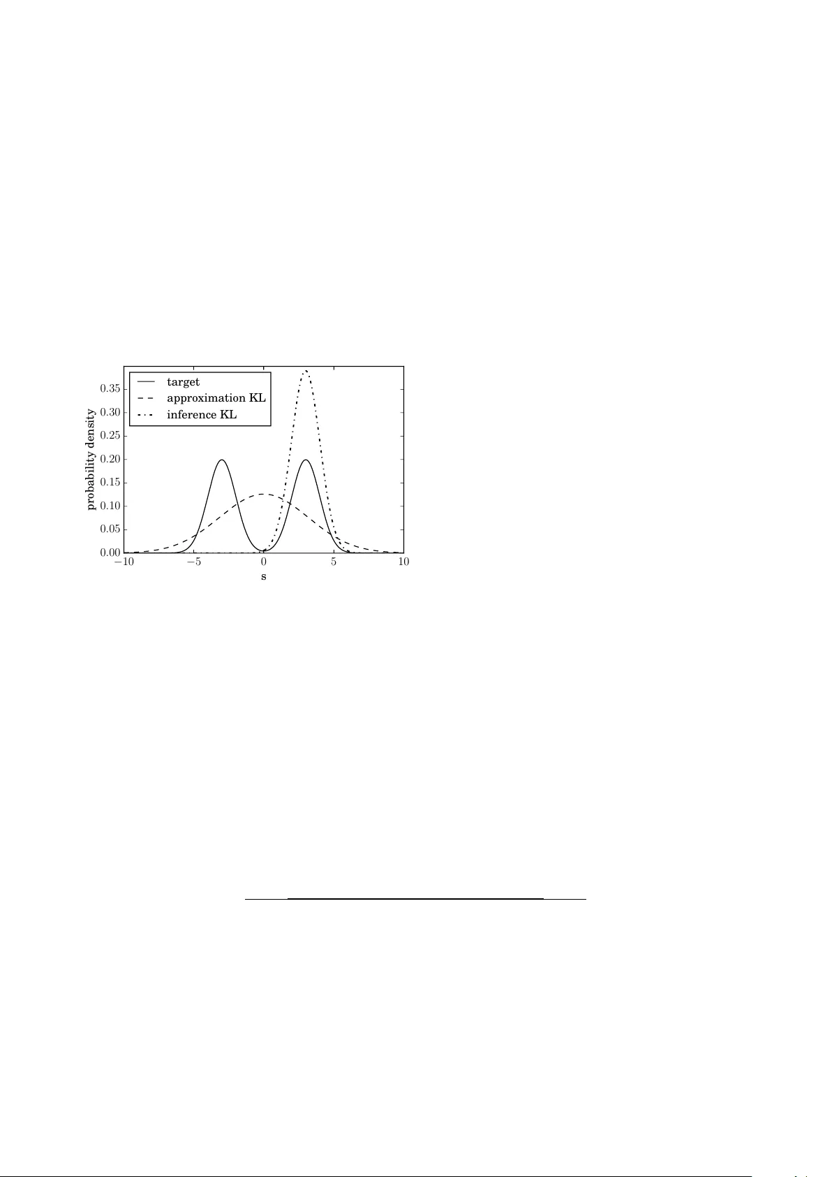
Optimal Belief Appro ximation Reimar H. Leik e, T orsten A. Enßlin Max-Planck-Institut f¨ ur Astr ophysik, Karl-Schwarzschildstr. 1, 85748 Gar ching, Germany Ludwig-Maximilians-Universit¨ at M¨ unchen, Geschwister-Schol l-Platz 1, 80539 Munich, Germany In Ba y esian statistics probabilit y distributions express b eliefs. How ev er, for many problems the b eliefs cannot be computed analytically and appro ximations of b eliefs are needed. W e seek a loss function that quantifies ho w “embarrassing” it is to comm unicate a given appro ximation. W e repro- duce and discuss an old pro of showing that there is only one ranking under the requirements that (1) the b est rank ed approximation is the non-appro ximated belief and (2) that the ranking judges appro ximations only by their predictions for actual outcomes. The loss function that is obtained in the deriv ation is equal to the Kullback-Leibler divergence when normalized. This loss function is frequen tly used in the literature. Ho wev er, there seems to be confusion about the correct order in whic h its functional argumen ts—the appro ximated and non-appro ximated beliefs—should be used. The correct order ensures that the recipient of a communication is only deprived of the minimal amoun t of information. W e hop e that the elemen tary deriv ation settles the apparen t confusion. F or example when approximating b eliefs with Gaussian distributions the optimal appro ximation is giv en b y momen t matching. This is in contrast to man y suggested computational sc hemes. Keywords: information theory , Bay esian inference, loss function, axiomatic deriv ation, mac hine learning I. INTR ODUCTION In Bay esian statistics, probabilities are interpreted as degrees of b elief. F or any set of mutually exclu- siv e and exhaustiv e even ts, one expresses the state of kno wledge as a probabilit y distribution ov er that set. The probabilit y of an even t then describ es the p er- sonal confidence that this even t will happ en or has happ ened. As a consequence, probabilities are sub- jectiv e prop erties reflecting the amoun t of knowledge an observ er has ab out the ev en ts; a differen t observ er migh t know which ev ent happened and assign differ- en t probabilities. If an observ er gains information, she up dates the probabilities she had assigned before. If the set of p ossible m utually exclusive and ex- haustiv e even ts is infinite, it is generally imp ossible to store all entries of the corresp onding probability dis- tribution on a computer or comm unicate it through a c hannel with finite bandwidth. One therefore needs to approximate the probabilit y distribution whic h de- scrib es one’s b elief. Given a limited set X of approx- imativ e b eliefs q ( s ) on a quan tity s , what is the b est b elief to approximate the actual b elief as expressed by the probability p ( s )? In the literature, it is sometimes claimed that the b est approximation is given by the q ∈ X that min- imizes the Kullback–Leibler divergence (“approxima- tion” KL) [1] KL( p, q ) = X s p ( s ) ln  p ( s ) q ( s )  (1) where q is the approximation and p is the real b elief. W e refer to this functional as “approximation” KL to emphasize its role in approximation, which will be de- riv ed in the course of this pap er and to distinguish it from the same functional, with q b eing a prior b e- lief and p being the p osterior b elief to which this KL is minimized in inference. W e will refer to the func- tional with q b eing the input and p obtained through minimization as “inference KL”. In Equation (1), min- imization is done with respect to its second argument. The deriv ation of this particular functional form v aries from field to field. F or example, in co ding theory , one tries to mini- mize the amoun t of bandwidth needed to transmit a message. Giv en a prior q ov er the sym b ols that the message consists of, an optimal scheme can b e derived. The approximation KL gives the exp ected amount of extra bits needed to transmit such a message if the sym b ols are actually drawn from the probability dis- tribution p instead of q [2]. If we kno w that p is the real probability distribution, the b est approximativ e probabilit y distribution q ∈ X to base a co ding on is therefore the one minimizing the approximation KL. Ho wev er, it is not clear that minimizing the amoun t of bits transferred is the b est or even only measure expressing how goo d such an approximation is in gen- eral. In machine learning and deep learning, neural net- w orks are trained to understand abstract data d ; for example, to assign a lab el s to it. This task can b e view ed as fitting an appro ximative probabilit y distri- bution q ( s | d ) to a true generating probabilit y distri- bution p ( s | d ). F or this, the approximativ e probabil- it y distribution is parametrized (to a neural net work) and then matched to the true, generating probability distribution using a loss function and samples. The most frequently used loss function is the cross entrop y , whic h is equiv alen t to the approximation KL. The rea- son to use this form is often either inspired from co d- ing theory , or by experimental exp erience [3]. Another argument for minimizing the approxima- tion KL is giv en in Chapter 13 of Reference [4], where it is claimed that this yields the maximum lik eliho od estimation to p ( s ) among the probability distribu- tions in X and that it giv es an unbiased and unique appro ximation. Interc hanging the arguments of the Kullbac k–Leibler divergence (the inference KL used in v ariational Bay es) generally leads to a biased esti- mate and do es not necessarily yield a unique result. These argumen ts undoubtedly give evidence for why minimizing the approximation KL gives a go o d esti- mate. How ev er, this do es not exclude all other meth- o ds. Ha ving an un biased estimate refers to getting the right mean. In our picture, this is a result of 2 optimal appro ximation and not a requirement for op- timalit y . Additionally , this result was derived with the help of information geometry , whose applicabil- it y to non-local problems is criticized, for example, in References [5, 6]. Con trary to the evidence for minimizing the appro x- imation KL, w e find man y examples where an approx- imation is made b y minimizing other functionals; for example, minimizing the inference KL (e.g., [7 – 13]). F or man y but not all of them, this is b ecause mini- mizing the appro ximation KL is not feasible in prac- tice in their case due to the real distribution p not b eing accessible. In this pap er, we seek to bring together the differ- en t motiv ations and give a full and consisten t picture. The pro of w e present here is not new; it goes back to [14], where there is an exact mathematical deriv ation for probabilit y densities analogously to our deriv ation. Ho wev er, there are earlier publications dealing with the discrete case [15 – 17]. Although this pro of dates bac k at least 40 years, its implication on appro ximat- ing b eliefs seem to b e quite unkno wn—esp ecially in the comm unit y of physicists applying Bay esian meth- o ds. In this pap er, w e repro duce a slightly mo dified v ersion of this pro of, giv e the result a new interpreta- tion and add further justification for the prerequisites used, laying emphasis on wh y one has to accept the ax- ioms necessary for the deriv ation if one is a Bay esian. W e provide argumentation for w h y b elieve approxi- mation is an imp ortant and omnipresen t topic. W e la y the emphasis of this pap er more on inter- pretation of results and justification of prerequisites, and thus present an easy version of the pro of where the loss function is assumed to b e differentiable. The pro of can how ever be extended to the general case of non-differen tiable loss [18]. The argumen t we repro- duce gives evidence that minimizing the approxima- tion KL is the b est approximation in theory . This argumen t do es not rest on information geometry nor is it restricted to coding theory . By imposing t wo con- sistency requiremen ts, one is able to exclude all rank- ing functions with the exception of one for ranking the appro ximative probability distributions q ∈ X . F or this, one employs the principle of loss functions [19], also called cost functions, regret functions, (or with flipp ed sign, utilit y functions or score functions) and sho ws that the unique loss function for ranking appro ximated probabilit y distributions is the approx- imation KL. F or us, a ranking is a total order in- dicating preference, whereas a loss is a map to R , whic h induces a ranking but additionally giv es an ab- solute scale to compare preferences. The presen ted axiomatic deriv ation do es not give rise to any new metho d, but it enables a simple chec king for whether a certain app roximation is most optimally done through the approximation KL. There are many other exam- ples of axiomatic deriv ations seeking to supp ort infor- mation theory on a fundamental level. Some notable examples are Co x deriv ation [20] of Ba yesian proba- bilit y theory as a unique extension of Bo olean algebra as well as a scien tific discussion on the maxim um en- trop y principle [21 – 23], establishing the inference KL as unique inference to ol (which ga ve rise to the naming con ven tion in this pap er). Most of these arguments rely on page-long proofs to arriv e at the Kullbac k– Leibler divergence. The pro of that is sketc hed in this pap er is only a few lines long, but nonetheless stan- dard literature for axiomatic deriv ation in Bay esian- ism do es not cite this “easy” deriv ation (e.g., the influ- en tial Reference [21]). As already discussed, approx- imation is an imp ortan t and unav oidable part of in- formation theory , and with the axiomatic deriv ation presen ted here we seek to provide orientation to sci- en tists searching for a wa y to approximate probabil- it y distributions. In Section I I, w e introduce the concept of loss func- tions, which is used in Section II I to define an op- timal scheme for approximating probabilit y distribu- tions that express b eliefs. W e briefly discuss the rel- ev ance of our deriv ations for the scien tific comm unit y in Section IV. W e conclude in Section V. I I. LOSS FUNCTIONS The idea to ev aluate predictions based on loss func- tions dates bac k 70 years, and w as first in tro duced by Brier [24]. W e explain loss functions by the means of parameter estimation. Imagine that one would like to giv e an estimate of a parameter s that is not known, whic h v alue of s should b e tak en as an estimate? One w ay to answer this question is b y using loss functions. F or this note that p ( s ) is now formally a probability measure, ho w ev er w e choose to write ´ d sp ( s ) instead of ´ d p ( s ) as if p ( s ) w ould b e a probability density . A loss function in the setting of parameter estimation is a function that takes an estimate σ for s and quan- tifies how “embarrassing” this estimate is if s = s 0 turns out to b e the case: L ( σ, s 0 ) The exp ected embarrassmen t can b e c omputed by using the knowledge p ( s ) about s : h L ( σ, s 0 ) i p ( s 0 ) = ˆ d s 0 L ( σ, s 0 ) p ( s 0 ) The next step is to take the estimate σ that min- imizes the exp ected embarr assment; that is, the ex- p ectation v alue of the loss function. F or differen t loss functions, one arriv es at different recip es for how to extract an estimate σ from the belief p ( s ); for exam- ple, for s ∈ R : L ( σ, s 0 ) = =          − δ ( σ − s 0 ) ⇒ T ak e σ such that p ( s ) | s = σ is maximal | σ − s 0 | ⇒ T ak e σ to b e the median ( σ − s 0 ) 2 ⇒ T ak e σ to b e the mean (2) In the context of parameter estimation, there is no general loss function that one should tak e. In man y scien tific applications, the third option is fav ored, but differen t situations might enforce differen t loss func- tions. In the con text of probability distributions, one 3 has a mathematical structure av ailable to guide the c hoice. In this con text, one can restrict the p ossibili- ties by requiring consisten t loss functions. I I I. THE UNIQUE LOSS FUNCTION Ho w embarrassing is it to appro ximate a probabilit y distribution b y q ( s ) ev en though it is actually p ( s )? W e quantify the em barrassmen t in a loss function L  q m , s 0  (3) whic h says ho w em barrassing it is to tell someone q ( s ) is one’s b elief ab out s in the ev ent that later s is mea- sured to b e s 0 . Here m is introduced as reference measure to make L coordinate indep endent. F or a finite set co ordinate indep endence is trivially fulfilled and it migh t seem that ha ving a reference measure m is sup erficial. Note how ev er, that it is a sensible additional requirement to ha ve the quantification b e in v arian t under splitting of ev ents, i.e. mapping to a bigger set where tw o now distinguishable ev ents rep- resen t one former large even t. The quotient q m is in- v arian t under such splitting of ev ents, whereas q itself is not. The reference measure m can b e any measure suc h that q is absolutely con tin uous with resp ect to m . Note further that we restrict ourselves to the case that we get to know the exact v alue of s . This do es not make our approach less general; imagining that w e would instead tak e a more general loss L ( q , ˜ q ( s )) where ˜ q is the knowledge ab out s at some later p oin t, then w e ma y define L  q m , s 0  = L ( q , δ ss 0 ) with δ de- noting the Kronec ker or Dirac delta function, and thus restrict ourselves again to the case of exact kno wledge. This line of reasoning w as sp elled out in detail by John Skilling [25]: “If there are general theories, then they m ust apply to special cases”. T o decide which b elief to tell someone, we lo ok at the exp ected loss D L  q m , s 0 E p ( s 0 ) = ˆ d s 0 L  q m , s 0  p ( s 0 ) (4) and try to find a q ∈ X that minimizes this exp ected loss. T o sum up, if w e are giv en a loss function, we ha ve a recip e for how to optimally appro ximate the b elief. Which loss functions are sensible, though? W e enforce t wo criteria that a go o d loss function should satisfy . Criterion 1 (Locality) If s = s 0 turne d out to b e the c ase, L only dep ends on the pr e diction q actual ly makes ab out s 0 : L  q m , s 0  = L  q ( s 0 ) m ( s 0 )  (5) Note that w e make an abuse of notation here, denot- ing the function on b oth sides of the equation by the same sym b ol. The criterion is called lo calit y b ecause it demands that the functional of q m should b e ev al- uated lo cally for every s 0 . It also forbids a direct dep endence of the loss L on s 0 whic h excludes losses that are a priori biased to wards certain outcomes s 0 . This form of lo cality is an intrinsically Bay esian prop ert y . Consider a situation where one w ants to decide whic h of tw o riv aling h ypotheses to believe. In order to distinguish them, some data d are measured. T o up date the prior using Bay es theorem, one only needs to kno w how probable the me asur e d data d are giv en each hypothesis, not how probable other p os- sible data ˜ d 6 = d that were not measured are. This migh t seem intuitiv e, but there exist hypothesis de- cision methods (not necessarily based on loss func- tions) that do not fulfill this prop erty . F or example, the non-Bay esian p -v alue depends mostly on data that w ere not measured (all the data that are at least as “extreme” as the measured data). Thus, it is a prop- ert y of Bay esian reasoning to judge predictions only b y using what was predicted ab out things that w ere measured. The second criterion is ev en more natural. If one is not restricted in what can b e told to others, then the b est thing should b e to tell them the actual b elief p . Criterion 2 (Optimalit y of the actual b elief, proper- ness.) L et X b e the set of al l pr ob ability distributions over s . F or al l p and al l m , the pr ob ability distribution q ∈ X with minimal exp e cte d loss is q = p : 0 =  ∂ ∂ q ( s ) D L  q m , s 0 E p  q = p (6) The last criterion is also referred to as a prop er loss (score) function in the literature; see Reference [26] for a mathematical o verview of differen t prop er scoring rules. Our version of this prop erty is sligh tly mo dified to the v ersion that is found in the literature as w e demand this optimum to b e obtained indep en- den tly of a reference measure m . There is a funda- men tal Ba yesian desiderata stating that “If there are m ultiple w a ys to arriv e at a solutions, then they m ust agree.” W e’d lik e to justify wh y this is a prop erty that is absolutely imp ortant. If one uses statistics as a to ol to answ er some question, then if that an- sw er would dep end on how statistics is applied, then this statistic itself is inconsistent. In our case, where the defined loss function is dep endent on an arbitrary reference measure m , the result is thus forced to b e indep enden t of that m . Note furthermore that although in tuitiv ely w e w ant the global optimum to be at the actual b elief p (re- ferred to as strictly prop er in the literature), mathe- matically we only need it to b e an extreme v alue for our deriv ation. Ha ving these tw o consistency requiremen ts fixed, we deriv e whic h kind of consistent loss functions are pos- sible. W e insert Equation (5) in to Equation (6), ex- pand the domain of the loss function to not necessarily normalized p ositive v ectors q ( s ) but in tro duce λ as a Lagrange multiplier to account for the fact that we minimize under the constraint of normalization. W e 4 compute 0 =  ∂ ∂ q ( s ) ´ d s 0  L  q ( s 0 ) m ( s 0 )  p ( s 0 ) + λ q ( s 0 )  q = p = ´ d s 0 ∂ L  p ( s 0 ) m ( s 0 )  δ ( s − s 0 ) m ( s 0 ) p ( s 0 ) + λ δ ( s − s 0 ) = ∂ L  p ( s ) m ( s )  p ( s ) m ( s ) + λ ⇒ ∂ L  p ( s ) m ( s )  = − λm ( s ) p ( s ) (7) Here ∂ L denotes the deriv ativ e of L . In the next step we substitute x := p ( s ) m ( s ) for the quotien t. Note that Equation (7) holds for all p ositive real v alues of x ∈ R + since the requested measure indep endence of the resulting ranking p ermits to insert any measure m . W e then obtain ∂ L ( x ) = − λ x ⇒ L ( x ) = − C ln ( x ) + D (8) where C > 0 and D are constants with resp ect to q . Note that through the t wo consistency requiremen ts one is able to completely fix what the loss function is. In the original pro of of [14], there arises an additional p ossibilit y for L if the sample space consists of 2 el- emen ts. In that case, the lo cality axiom, as it is used in the literature, do es not constrain L at all. In our case, where w e introduced m as a reference measure, w e are able to exclude that p ossibility . Note that the constan ts C and D are irrelev an t for determining the optimal approximation as they do not affect where the minim um of the loss function is. T o sum up our result if one is restricted to the closed set X of probability distributions, one should take that q ∈ X that minimizes D L  q m , s 0 E p ( s 0 ) = − ˆ d s 0 p ( s 0 ) ln  q ( s 0 ) m ( s 0 )  (9) in order to obtain the optimal approximation, where it is not imp ortant what m is used. If one takes m = 1, this loss is the cross entrop y h− ln ( q ( s 0 )) i p ( s 0 ) . If one desires a rating of how goo d an approxima- tion is, and not only a ranking which appro ximation is best, one could go one step further and enforce a third criterion: Criterion 3 (zero loss of the actual b elief ) F or al l p , the exp e cte d loss of the pr ob ability distribution p is 0: 0 = D L  p m , s 0 E p (10) This criterion trivially forces m = p and makes the quan tification unique while inducing the same rank- ing. Thus w e arriv e at the Kullback-Leibler div ergence KL( p, q ) = ˆ d s 0 p ( s 0 )ln  p ( s 0 ) q ( s 0 )  as the optimal rating and ranking function. T o phrase the result in words, the optimal wa y to appro ximate the b elief p is such that given the appro x- imated b elief q , the amount of information KL( p, q ) that has to be obtained for someone who b elieves q to arrive back at the actual belief p is minimal. W e should mak e it as easy as p ossible for someone who got an appro ximation q to get to the correct b elief p . This sounds like a trivial statement, explaining why the approximation KL is already widely used for ex- actly that task. IV. DISCUSSION W e briefly discuss the implications of these results. In comparison to Reference [2, 4], we presen ted an- other more elementary line of argumentation for the claim that the appro ximation KL is the correct rank- ing function for approximating which holds in a more general setting. Other works that base their results on minimizing the inference KL (KL( q, p )) for b elief approximation are not optimal with resp ect to the ranking function w e deriv ed in Section II I. One reason for preferring the for this purp ose non-optimal inference KL is that it is computationally feasible for many applications, in con trast to the optimal approximation. As long as the optimal sc heme is not computationally accessible, this argumen t has its merits. Another reason for minimizing the inference KL for appro ximation that is often cited (e.g., [27]) is that it giv es a low er b ound to the log-likelihoo d ln( p ( d | s )) =  ln  p ( d, s ) q ( s )  q ( s ) + KL( q , p ) (11) whic h for example giv es rise to the exp ectation maxi- mization (EM- ) algorithm [28]. How ev er, the metho d only gives rise to maximum a p osteriori or maximum lik eliho o d solutions, which corresp onds to optimizing the δ -loss of Equation (2). In Reference [11], it is claimed that minimizing the inference KL yields more desirable results since for m ulti-mo dal distributions, individual mo des can b e fitted with a mono-mo dal distribution such as a Gaus- sian distribution, whereas the resulting distribution has a v ery large v ariance when minimizing the ap- pro ximation KL to account for all mo des. In Figure 1 there is an example of this b eha vior. The true distri- bution of the quantit y s is tak en to be a mixture of t wo standard Gaussians with means ± 3. It is appro x- imated with one Gaussian distribution by using the appro ximation KL and the inference KL. When using the appro ximation KL, the resulting distribution has a large v ariance to cov er b oth p eaks. Minimizing the inference KL leads to a sharply peaked approxima- tion around one p eak. A user of this metho d migh t b e very confident that the v alue of s must b e near 3, ev en though the result is heavily dependent on the initial condition of the minimization and could hav e b ecome p eak ed around − 3 just as w ell. W e find that fitting a m ulti-mo dal distribution with a mono-mo dal one will yield sub optimal results ir- resp ectiv e of the fitting sc heme. An approximation should alw ays hav e the goal to b e close to the target that is b eing appro ximated. If it is already apparen t that this goal cannot b e achiev ed, it is recommended 5 to rethink the set of appro ximative distributions and not dwell on the algorithm used for approximation. In Reference [12] an approximativ e simulation sc heme called information field dynamics is described. There, a Gaussian distribution q is matched to a time-ev olved v ersion U ( p ) of a Gaussian distribution p . This matc hing is done by minimizing the infer- ence KL. In this particular case (at least for infor- mation preserving dynamics), the matching can b e made optimal without making the algorithm more complicated. Since for information preserving dy- namics time ev olution is just a change of co ordinates and the Kullback–Leibler divergence is inv ariant un- der such transformations, one can instead match the Gaussian distribution p and U − 1 ( q ) by minimizing KL( p, U − 1 ( q )) = KL( U ( p ) , q ), which is just as diffi- cult in terms of computation. − 10 − 5 0 5 10 s 0 . 00 0 . 05 0 . 10 0 . 15 0 . 20 0 . 25 0 . 30 0 . 35 probability density target approximation KL inference KL Figure 1: Results of approximating a target distribution in s with a Gaussian distribution. KL: Kullbac k–Leibler. In Reference [13] it is claimed that the inference KL yields an optimal approximation scheme fulfilling cer- tain axioms. This result is the exact opp osite of our result. This disagreement is due to an assumed con- sistency of approximations. In Reference [13], further appro ximations are forced to b e consistent with earlier appro ximations; i.e., if one do es t w o approximations, one gets the same result as with one joint approxima- tion. Due to this requiremen t, the derived functional cannot satisfy some of the axioms that we used. In our picture, it is b etter to do one large approxima- tion instead of many small approximations. This is in accordance to the behavior of other approximations. F or example, when step-wise rounding the real n um- b er 1 . 49, one gets 2 if it is first rounded to one deci- mal and then to integer precision compared to b eing rounded to integer precision directly where one gets 1. If information is lost due to appro ximation, it is natural for further appro ximations to b e less precise than if one were to appro ximate in one go. There also exist cases where w e could not find an y comments explaining wh y the arguments of the Kullbac k–Leibler div ergence are in that particular or- der. In general, it would b e desirable that authors pro vide a short argumentation for wh y they choose a particular order of the arguments of the KL diver- gence. V. CONCLUSIONS Using the t wo elementary consistency requiremen ts on locality and optimality , as expressed by Equations (5) and (6), respectively , we hav e shown that there is only one ranking function that ranks how go o d an approximation of a b elief is, analogously to Ref- erence [14]. By minimizing KL( p, q ) with resp ect to its second argument q ∈ X , one gets the b est appro x- imation to p . This is claimed at sev eral p oints in the literature. Nev ertheless, w e found sources where other functionals w ere minimized in order to obtain an ap- pro ximation. This confusion is probably due to the fact that for the slightly different task of up dating a b elief q under new constrain ts, KL( p, q ) has to b e min- imized with resp ect to p , its first argument [29, 30]. W e do not claim that any of the direction of Kullbac k– Leibler divergence are wrong by themselv es, but one should b e careful of when to use whic h. W e hop e that for the case of appro ximating a prob- abilit y distribution p by another q we hav e given con- vincing and conclusive arguments for why this should b e done by minimizing KL( p, q ) with resp ect to q , if this is feasible. VI. A CKNOWLEDGEMENTS W e would lik e to thank A. Catic ha, J. Skilling, V. B¨ ohm, J. Knollm ¨ uller, N. P orqueres, and M. Greiner and six anonymous referees for the discussions and their v aluable commen ts on the manuscript. [1] S. Kullback and R. Leibler, Annals of Mathematical Statistics 22 (1) , 79 (1951). [2] T. M. Cov er and J. A. Thomas, (2006). [3] I. Go o dfellow, Y. Bengio, and A. Courville, De ep L e arning (MIT Press, 2016) http://www. deeplearningbook.org . [4] M. Opp er and D. Saad, A dvanc e d me an field metho ds: The ory and pr actic e (MIT press, 2001). [5] J. Skilling, in BA YESIAN INFERENCE AND MAX- IMUM ENTROPY METHODS IN SCIENCE AND ENGINEERING: Pr o c e e dings of the 33r d Interna- tional Workshop on Bayesian Infer enc e and Maxi- mum Entr opy Metho ds in Scienc e and Engine ering (MaxEnt 2013) , V ol. 1636 (AIP Publishing, 2014) pp. 24–29. [6] J. Skilling, in Bayesian infer enc e and maximum en- tr opy metho ds in scienc e and engineering (MAXENT 2014), e ds. A. Mohammad-Djafari and F. Barb ar esc o, AIP Confer enc e Pro c e e dings , V ol. 1641 (2015) pp. 27– 42. [7] C. W. F ox and S. J. Rob erts, Artificial intelligence review 38 , 85 (2012). 6 [8] T. A. Enßlin and C. W eig, Ph ys. Rev. E 82 , 051112 (2010), arXiv:1004.2868 [astro-ph.IM]. [9] D. M. Blei, A. Kucukelbir, and J. D. McAuliffe, ArXiv e-prin ts (2016), arXiv:1601.00670 [stat.CO]. [10] F. J. Pinski, G. Simpson, A. M. Stuart, and H. W eb er, ArXiv e-prin ts (2014), [math.NA]. [11] F. Pinski, G. Simpson, A. Stuart, and H. W eb er, ArXiv e-prin ts (2013), arXiv:1310.7845 [math.PR]. [12] T. A. Enßlin, Ph ys. Rev. E 87 , 013308 (2013), arXiv:1206.4229 [physics.comp-ph]. [13] C.-Y. Tseng and A. Catic ha, Physica A Statistical Mec hanics and its Applications 387 , 6759 (2008), arXiv:0808.4160 [cond-mat.stat-mech]. [14] J. M. Bernardo, The Annals of Statistics , 686 (1979). [15] J. Acz ´ el and J. Pfanzagl, Metrik a 11 , 91 (1967). [16] J. McCarth y , Pro ceedings of the National Academy of Sciences 42 , 654 (1956). [17] I. J. Go o d, Journal of the Roy al Statistical So ciety . Series B (Metho dological) , 107 (1952). [18] P . Harremo ¨ es, arXiv preprin t (2017). [19] H. Cram´ er, On the mathematic al the ory of risk (Cen- traltryc keriet, 1930). [20] R. T. Cox, American Journal of Physics 14 , 1 (1946). [21] E. T. Jaynes, Pr ob ability The ory, by E. T. Jaynes and Edite d by G. L arry Br etthorst, pp. 758. ISBN 0521592712. Cambridge, UK: Cambridge University Pr ess, June 2003. , edited by Bretthorst, G. L. (2003). [22] J. Skilling, in Maximum-Entr opy and Bayesian Meth- o ds in Scienc e and Engine ering (Springer, 1988) pp. 173–187. [23] A. Caticha, in Bayesian Infer enc e and Maximum En- tr opy Metho ds in Scienc e and Engine ering , Ameri- can Institute of Physics Conference Series, V ol. 707, edited b y G. J. Eric kson and Y. Zhai (2004) pp. 75–96, ph ysics/0311093. [24] G. W. Brier, Mon thly w eather review 78 , 1 (1950). [25] J. Skilling, in Maximum entr opy and Bayesian meth- o ds (Springer, 1989) pp. 45–52. [26] T. Gneiting and A. E. Raftery , Journal of the Amer- ican Statistical Asso ciation 102 , 359 (2007). [27] C. Bishop, Pattern R e c o gnition and Machine L e arning (Information Scienc e and Statistics), 1st e dn. 2006. c orr. 2nd printing e dn (2007). [28] A. P . Dempster, N. M. Laird, and D. B. Rubin, Jour- nal of the roy al statistical so ciet y . Series B (method- ological) , 1 (1977). [29] I. Csiszar, The annals of statistics , 2032 (1991). [30] A. Catic ha, ArXiv e-prints (2014),