Latent common manifold learning with alternating diffusion: analysis and applications

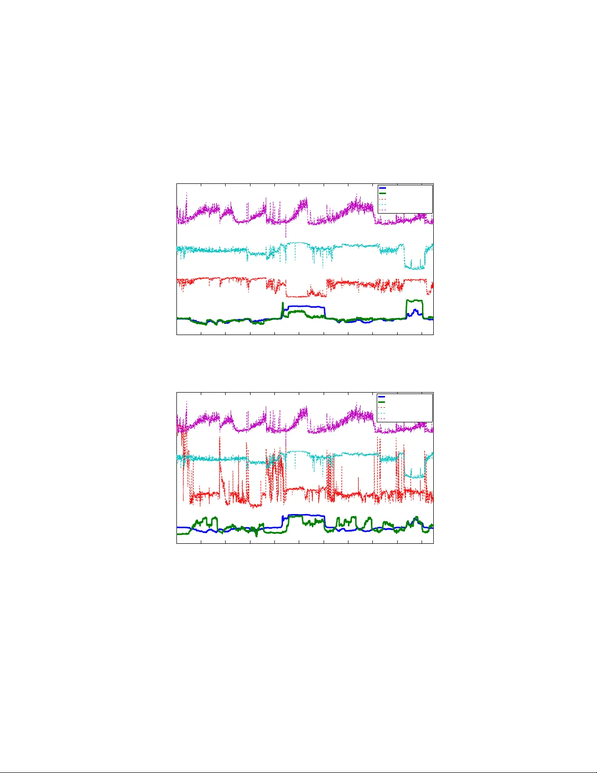
Latent common manifold learning with alternating dif fusion: analysis and applications Ronen T almon a , Hau-T ieng W u b,c a V iterbi F aculty of Electrical Engineering, T echnion - Isr ael Institute of T echnology , Haifa, Isr ael b Department of Mathematics and Department of Statistical Science, Duke University , Durham, NC, USA c Mathematics Division, National Center for Theor etical Sciences, T aipei, T aiwan Abstract The analysis of data sets arising from multiple sensors has drawn signiﬁcant re- search attention ov er the years. T raditional methods, including kernel-based methods, are typically incapable of capturing nonlinear geometric structures. W e introduce a la- tent common manifold model underlying multiple sensor observations for the purpose of multimodal data fusion. A method based on alternating diffusion is presented and analyzed; we provide theoretical analysis of the method under the latent common man- ifold model. T o exemplify the power of the proposed frame work, experimental results in sev eral applications are reported. K e ywor ds: common manifold, alternating diffusion, sensor fusion, multimodal sensor , data fusion, seasonality , diffusion maps, manifold learning 1. Introduction One of the long-standing challenges in signal processing is the fusion of informa- tion acquired by multiple, multimodal sensors. The problem of information fusion has become particularly central in the wak e of recent technological advances, which have led to extensiv e collection and storage of multimodal data. No wadays, many devices and systems, e.g., cell-phones, laptops, and wearable-devices, incorporate more than one sensor , often of different types. Of particular interest in the context of this paper are the massi ve data sets of medical recordings and healthcare-related information, ac- quired routinely , for e xample, in operation rooms, intensi ve care units, and clinics. The av ailability of such distinct and complementary information calls for the development of ne w theories and methods, le veraging it to ward achieving concrete data analysis objectiv es, such as ﬁltering and prediction, in a broad range of ﬁelds. Problems in multimodal signal processing has been studied for many years and has been approached from v arious research directions [27]. A classic approach for such problems is Canonical Correlation Analysis (CCA) [22], which recov ers highly Email addr esses: ronen@ef.technion.ac.il (Ronen T almon), hauwu@math.duke.edu (Hau-T ieng W u) Pr eprint submitted to Elsevier August 4, 2017 correlated linear projections from two data sets. T o extend the linear setting and to address aspects of nonlinearities, CCA was applied in a kernel space (e.g., [28, 1]). Recently , ample work based on the optimization criterion of CCA and kernels has been presented, addressing multi-view problems, and in particular , using multi-kernel learning (e.g. [2, 29]) and a variety of manipulations and combinations of kernels, e.g. [5, 11, 10, 35, 36, 51, 25, 3, 23, 50, 48, 33, 34, 17, 38]. Our exposition begins by addressing a particular baseline problem. Consider mul- tiple sensors measuring the same physical phenomenon, such that the properties of the physical phenomenon are manifested as a hidden manifold (which we w ould lik e to e x- tract), while each sensor presents its own deformation and has its own sensor-speciﬁc effects (hidden nuisance variables, which we would like to suppress). W e assume that the relations between the measurements and the nuisance variables are unknown. The goal is to uncover the common latent manifold and to suppress the sensor-speciﬁc vari- ables, thereby e xtracting the essence of the data and separating the relev ant information from the irrelev ant information. This baseline problem highlights an important aspect in the analysis of multimodal data sets; that is, the sensor-related v ariables may not be strictly related to noise and interferences. Often, such variables exhibit “structures”, such as the position and ori- entation of the acquiring sensor, en vironmental effects, and channel characteristics. T o address this, we propose an approach based on manifold learning. The power of manifold learning can be exploited in this setting, since it is designed to capture non- linear topological and geometric structures underlying data, and it does not require prior model knowledge, which can be particularly hard to obtain in the case of mul- tiple modalities. Manifold learning is a class of nonlinear data-driv en methods, e.g. [47, 42, 14, 4], often used to extract the underlying structures in a given data set. Of particular interest in the context of this paper is diffusion map (DM), [6], in which discrete diffusion processes are constructed on the giv en data points; these diffusion processes are designed to capture the geometry of the underlying variability in a single data set. Multimodal data present a challenge to such a geometric analysis approach, since multiple sensors often lead to undesired geometric structures stemming from the div ersity of the different acquisition techniques used in the sensors, making it more difﬁcult to identify and e xtract only the “important” variables. Nev ertheless, multiple data sets from various sensors encompass more information, and therefore, enable us to recover a more reliable description of the measured (physical) phenomenon. Based on manifold learning, se veral methods have been proposed to analyze simultaneously multiple data sets. One approach is to concatenate the vectors representing each data set into one vector [8]; ho wev er , the question of ho w each data set should be scaled and concatenated naturally arises, especially if the data sets are acquired by very dif ferent modalities. T o address such scaling aspects, it has been proposed in [24] to use DM to obtain a low-dimensional “standardized” representation of each data set, and then to concatenate these representations. Ho wev er , such methods aggre gate all the variables from all the giv en data sets, and they neither distinguish the important information nor discard the sensor-speciﬁc v ariables. Our research direction in volving geometric analysis encompasses several signiﬁ- cant advantages. First, the method we present is data-driv en and “model-free” in the sense that in addition to the manifold assumption, it does not rely on prior kno wledge. 2 In multimodal problems, this is an important advantage, since it circumvents the need to design an appropriate model for each modality , as well as the “hard wiring” required for the fusion of different data sets. Second, manifold learning methods are typically formulated in general settings, and therefore, do not require strong assumptions on the nature of the data or on the nature of the sensors. As a result, our method is restricted to neither certain applications nor to multi-view problems, consisting of data acquired only by a single type of sensors. Third, the combination of geometric analysis, en- abling to inte grate subtle patterns and structures underlying data, and the av ailability of multiple data sets providing complementary information, gives rise to the discovery of intrinsic structures. Furthermore, the diffusion approach has been sho wn to be rob ust to noise [15, 16], and hence allows us to devise a reliable approach for extracting the interesting information from highly noisy data. Recently , a data-driv en method to recover the common latent variable underlying multiple, multimodal sensor data based on alternating products of diffusion operators was presented [30, 31]; we refer to this method as alternating diffusion (AD). It was shown both theoretically and in illustrative examples (with real recordings) that this method extracts useful information about the common source of variability in a multi- sensor experiment as if it were a typically diffusion operator applied directly to data sampled from only the interesting/common source of v ariability . The formulation and analysis in [30] are based on a setting including only metric spaces and the common source of variability is identical in the dif ferent sensors. In the current w ork, we extend [30] and enhance the theoretical results by explicitly introducing a setting with a common manifold , which can be well accessed by different sensors, while different types of deformations are introduced due to various effects of the speciﬁc sensors. W e focus on the case in which there is a common manifold underlying all the giv en data sets, and propose a data-driv en method for recovering the common manifold and constructing its representation. More speciﬁcally , in an analogous way to the classic diffusion geometry approach [6], we show that by using a product of dif fusion operators in DM, we are able to approximate a modiﬁed/deformed Laplace operator on the underlying common manifold. Our main contribution in this paper can be summarized as follo ws. (i) While most current manifold learning methods only address a single data set arising from a sin- gle manifold, we extend this basic setting and present a technique addressing sev eral data sets arising from multiple manifolds. (ii) W e introduce a new concept of “nonlin- ear manifold ﬁltering”, that is, removing the inﬂuence of the nuisance variables, with a rigorous theoretical foundations and analysis. (iii) The ability to extract the com- mon manifold underlying se veral data sets enables us to propose new methods for the multimodal sensor fusion problem. These methods consist of a scheme to incorporate nonlinear geometric priors into a manifold ﬁltering procedure and are demonstrated on illustrative (real) examples. Speciﬁcally , we sho w application to the analysis of sleep dynamics as well as to seasonal pattern detection (a problem which is commonly encountered in time series analysis and will be introduced in the sequel). The remainder of this paper is organized as follows. In Section 2, the common manifold model for multiple data sets collected from multimodal sensors is introduced. W ith the common manifold model, the AD algorithm is formulated and its analysis is provided. T o further study the beha vior of AD in the common manifold model, in Sec- 3 tion 3, asymptotical analysis results are pro vided. More details about the AD algorithm for practical purposes are discussed in Section 4. In Section 5, we e xploit the common manifold model and design an AD algorithm to detect seasonal patterns in time series. W e provide a seasonality index to quantify the seasonal effects. In Section 6, a sleep data set is studied, demonstrating the power of the common manifold model and the AD algorithm in the medical ﬁeld. W e will sho w that among different pairs of sensors, different physiological information is obtained. In Section 7, the prototypical exten- sion problem of manifold representations is considered and discussed for the common manifold model and the AD algorithm. Discussion and future directions are outlined in Section 8. The proofs of the theoretical results from Section 3 are presented in the Appendix. 2. Common Manifold Model and Alter nating Diffusion The success of the AD algorithm has been shown in different problems, for ex- ample, for sleep depth analysis [31]. T o analyze the algorithm, in [30], the common variable as well as the nuisance v ariables speciﬁc for each sensor are modeled by met- ric measure spaces; speciﬁcally , it is shown that the diffusion distance calculated from the data via AD is equiv alent to an “ef fectiv e alternating-diffusion distance”, which is deﬁned only on one common variable shared by the two sensors [30, Theorem 5 and Equation 79]. Howe ver , in some problems, the data may exhibit additional structures, which could be extracted and exploited. In this paper , we consider such a case where the common v ariable has a distinct geometric structure, which is modelled by a man- ifold. Y et, e ven if we assume that the system we observe remains ﬁxed during the observation, the data collected from different sensors might depend on the observation procedure or be contaminated by different irrelev ant information. In particular, the common manifold might be deformed differently by dif ferent sensors. As a result, spe- cial focus is giv en to possible dependencies between the “common manifold” and the sensors. These considerations are manifested in the setting presented in this section, and our focus in the remainder of the paper is on studying the geometric information that can be obtained from AD. 2.1. Common manifold model Consider a setup consisting of multiple sensors observing a system or a phenomenon of interest simultaneously . T o simplify the e xposition, we focus on a setup with merely two sensors, noting that our analysis can be generalized to multiple sensors with slight modiﬁcations. 2.1.1. Geometric model Suppose there exists a common structure underlying the two sensor observations, which is modeled by a low dimensional common manifold , and suppose that each sen- sor introduces various deformations and interferences, which are modeled by other irrelev ant nuisance structures. Mathematically , denote the common structure of inter- est, M , by a d -dim Riemannian manifold with the metric tensor g ( i ) , which depends on the sensor , where i = 1 , 2 is the sensor inde x, and let d g ( i ) denote the distance function 4 The$ Underly ing$ Spac e$St ruct ure$ Sen so r Sen so r N 1 N 2 M S 1 S 2 s (1) s (2) Figure 1: A diagram illustrating our setting with a common manifold underlying two sensor observ ations. on M associated with g ( i ) . T o accommodate possible discrepancies and deformations between the common manifold observ ed through the tw o sensors, we allow the metrics to be dif ferent, i.e., g (1) 6 = g (2) . For i = 1 , 2 , let N i be a compact metric space with the distance function d N i , which models the irrele vant nuisance structures. Let S i denote the observable metric space with the distance function d S i , which models the space of the collected/accessible data by the i -th sensor . Assume that s ( i ) : M × N 1 × N 2 → S i (1) is a smooth isometric embedding of M × N i into S i modeling ho w the i -th sensor collects data, where i = 1 , 2 . Importantly , note that s (1) ignores N 2 (as it represents the interferences speciﬁc to the the second sensor), and that s (2) ignores N 1 (as it represents the interferences speciﬁc to the ﬁrst sensor). In other words, each sensor typically acquires two structures: a deformation of the common manifold of interest and an additional nuisance structure. The model described here implies that we do not hav e access to the structures underlying each sensor (the deformed common manifold M i and the nuisance structure N i ), nor to the mapping to the observ able sensor space (1). In addition, (1) means that for ( x, y, z ) , ( x 0 , y 0 , z 0 ) ∈ M × N 1 × N 2 , where x, x 0 ∈ M , y , y 0 ∈ N 1 and z , z 0 ∈ N 2 , we hav e d S 1 ( s (1) ( x, y , z ) , s (1) ( x 0 , y 0 , z 0 )) 2 = d g (1) ( x, x 0 ) 2 + d N 1 ( y , y 0 ) 2 (2) d S 2 ( s (2) ( x, y , z ) , s (2) ( x 0 , y 0 , z 0 )) 2 = d g (2) ( x, x 0 ) 2 + d N 2 ( z , z 0 ) 2 . In practice, we do not have the full access to the metric structure (2), but only to the observable distance functions d S i . In summary , different sensors hav e access to the information of interest from the 5 common geometric object M . Howe ver , the acquired information is deformed by two different sources – the nuisance variables modeled by N i , and the deformation induced by each sensor modeled by the different metric on the manifold M . A diagram of the geometric model is depicted in Figure 1. 2.1.2. Statistical model T o model the discrete data sets collected by the sensors, let (Ω , F , P ) be a probabil- ity space, where Ω is the e vent space, F is the sigma algebra on Ω , and P is a probabil- ity measure deﬁned on F . Consider a random vector S : (Ω , F , P ) → M × N 1 × N 2 . The dataset sampled from the i -th sensor , i = 1 , 2 , is modeled by a random vector S i = s ( i ) ◦ S . Note that via the ﬁrst sensor, only M and N 1 are observed in S 1 , while via the second sensor , only M and N 2 are observed in S 2 . W e further assume that conditional on M , the nuisance variables modeled by N 1 and N 2 (introduced by the different sensors) are sampled independently . Let ν := ν M×N 1 ×N 2 = S ∗ P denote the induced probability measure on M × N 1 × N 2 . By the assumption that conditional on M the nuisance v ariables are independent, we hav e ν ( x, y , z ) = ν M ( x ) ν N 1 |M ( y | x ) ν N 2 |M ( z | x ) , (3) where ν M ( x ) is the marginal distribution on M , and ν N i |M ( ·| x ) is the conditional distribution on N i . T o enhance the readability of the paper , we summarize the notations in T able 1. 2.2. Alternating diffusion under the common manifold model Based on the common manifold model, we apply AD to analyze data collected si- multaneously from two sensors, possibly of dif ferent modalities. The goal is to extract the common manifold from the observed data via AD. Throughout the paper , we use three sets of notations. The ﬁrst set will be deﬁned on the accessible data, typically using an observ able k ernel and an observ able dif fusion. The second set is intermediate and designed to describe the relationship between the observation and the hidden com- mon manifold. The third set will be deﬁned on the hidden common manifold using an (inaccessible) effecti v e kernel and ef fectiv e diffusion. Deﬁnition 2.1 (Observable Diffusion Kernels) . Let ˜ P ( i ) ∈ C ([0 , ∞ )) , i = 1 , 2 , be two kernels that decay suf ﬁciently fast and ar e associated with the two sensors. Deﬁne ˜ P ( i )  (( x, y , z ) , ( z 0 , y 0 , z 0 )) := ˜ P ( i )  d S ( i ) ( s ( i ) ( x, y , z ) , s ( i ) ( x 0 , y 0 , z 0 )) √   (4) P ( i )  (( x, y , z ) , ( x 0 , y 0 , z 0 )) := ˜ P ( i )  (( x, y , z ) , ( x 0 , y 0 , z 0 )) R M×N 1 ×N 2 ˜ P ( i )  (( x, y , z ) , ( x 00 , y 00 , z 00 )) d ν ( x 00 , y 00 , z 00 ) . wher e P ( i )  is referr ed to as a diffusion kernel with bandwidth  associated with the observable metric measur e space S i = s ( i ) ( M × N 1 × N 2 ) . 6 Symbol ( i = 1 , 2 ) Meaning ( M , g ( i ) ) d -dim Riemannian manifold with the Riemannian metric g ( i ) ( N i , d N i ) Compact metric space with the metric d N i ( S i , d S i ) Metric space with the metric d S i s ( i ) Sensor collecting data  Bandwidth parameter of the kernel function D ( i ) Observable dif fusion operator on S i ˜ P ( i ) Kernel associated with D ( i ) D Observable AD operator starting from the ﬁrst sensor E Marginalization operator D ( e i ) Effecti v e diffusion operator on ( M , g ( i ) ) ˜ P ( e ) Kernel associated with D ( e i ) D ( e ) Effecti v e AD operator starting from the ﬁrst sensor ˜ P ( O i ,y ) Observable dif fusion kernel with the ﬁx ed y ι ( i ) Embed M into R p so that g ( i ) is the induced metric via ι ( i ) ˜ K ( i ) Diffusion k ernel on ( M , g ( i ) ) T Reduced AD operator starting from ( M , g (1) ) ˜ K ( e ) Kernel associated with T exp ( i ) x Exponential map at x ∇ ( i ) Levi-Ci vita connection associated with the metric g ( i ) d V ( i ) V olume form associated with the metric g ( i ) Ric ( i ) Ricci curvature of ( M , g ( i ) ) s ( i ) Scalar curvature of ( M , g ( i ) ) Π ( i ) second fundamental form of the embedding ι ( i ) ∆ ( i ) Laplace-Beltrami operator of ( M , g ( i ) ) T able 1: Summary of symbols used throughout the paper . Note that the diffusion k ernel P ( i )  is in a normalized form, i.e., Z M×N 1 ×N 2 P ( i )  (( x, y , z ) , ( x 0 , y 0 , z 0 )) d ν ( x 0 , y 0 , z 0 ) = 1 . The main beneﬁt of a diffusion k ernel in such a normalized form is that the normaliza- tion helps to eliminate unwanted non-intrinsic quantities, such as the terms depending on the speciﬁc kernel in the asymptotical analysis. See, for example, the difference between Lemma 8 and Proposition 10 in [6] 1 . For each kernel,  is referred to as the bandwidth of the kernel. Further note that while the bandwidth may depend on the sensor , for simplicity , we assume that the kernels share the same  v alue. In this section, we show that when studied under a suitable assumption, the inﬂu- 1 Note that in [30] the analysis is carried out using forward dif fusion, while in this paper we use backward diffusion for consistenc y with the standard diffusion maps frame work presented in [6]. 7 ence of the nuisance variables, that is, each metric space N i representing the sensor effects and observation speciﬁc inﬂuences, is erased by the AD procedure, and thus, can be ignored. Note that in the special case when g (1) = g (2) , i.e., the common man- ifold is viewed similarly by different sensors, this statement was sho wn previously in [30], where the focus is on the diffusion distance. W e begin with the follo wing deﬁnition. Deﬁnition 2.2 (Observable Dif fusion Operators) . F or a function f ∈ C ( M×N 1 ×N 2 ) , let D ( i ) : C ( M × N 1 × N 2 ) → C ( M × N 1 × N 2 ) , for i = 1 , 2 , denote the diffusion operator on the i -th sensor , deﬁned by D ( i ) f ( x, y , z ) := Z M×N 1 ×N 2 P ( i )  (( x, y , z ) , ( x 0 , y 0 , z 0 )) f ( x 0 , y 0 , z 0 ) d ν ( x 0 , y 0 , z 0 ) . (5) Deﬁnition 2.3 (Observable Alternating Dif fusion Operator and K ernel) . The AD oper - ator starting fr om the ﬁrst sensor is deﬁned by D := D (2) D (1) , (6) while the AD operator starting from the second sensor is deﬁned analogously . Let P  ∈ C (( M × N 1 × N 2 ) × ( M × N 1 × N 2 )) be the AD kernel , deﬁned by P  (( x, y , z ) , ( x 00 , y 00 , z 00 )) (7) := Z M×N 1 ×N 2 P (2)  (( x, y , z ) , ( x 0 , y 0 , z 0 )) P (1)  (( x 0 , y 0 , z 0 ) , ( x 00 , y 00 , z 00 )) d ν ( x 0 , y 0 , z 0 ) . Note that by deﬁnition, we can associate the observable AD k ernel and operator: ( D f )( x, y , z ) = Z M×N 1 ×N 2 P  (( x, y , z ) , ( x 00 , y 00 , z 00 )) f ( x 00 , y 00 , z 00 ) d ν ( x 00 , y 00 , z 00 ) . (8) The second set of notations concerns with the connection between the observations and the hidden common manifold. Consider the observable AD starting from the ﬁrst sensor , and recall that the ﬁrst sensor only sees M × N 1 . Thus, by the deﬁnition of ˜ P (1) in (2) and (4), P (1)  (( x, y , z ) , ( x 0 , y 0 , z 0 )) only takes ( x, y ) and ( x 0 , y 0 ) into account. W e thus introduce the corresponding reduced intermediate diffusion k ernels: ˜ P ( I 1 )  (( x 0 , y 0 ) , ( x 00 , y 00 )) := ˜ P (1)  (( x 0 , y 0 , z 0 ) , ( x 00 , y 00 , z 00 )) P ( I 1 )  (( x 0 , y 0 ) , ( x 00 , y 00 )) := P (1)  (( x 0 , y 0 , z 0 ) , ( x 00 , y 00 , z 00 )) ; (9) that is, the observable dif fusion starting from the ﬁrst sensor can be simpliﬁed by ig- noring the contribution of N 2 . Similarly , we deﬁne ˜ P ( I 2 )  (( x 0 , z 0 ) , ( x 00 , z 00 )) := ˜ P (2)  (( x 0 , y 0 , z 0 ) , ( x 00 , y 00 , z 00 )) P ( I 2 )  (( x 0 , z 0 ) , ( x 00 , z 00 )) := P (2)  (( x 0 , y 0 , z 0 ) , ( x 00 , y 00 , z 00 )) . (10) 8 Clearly , by deﬁntion, for f ∈ C ( M × N 1 × N 2 ) , D (1) f ( x, y , · ) is a constant function for a ﬁxed ( x, y ) . Accordingly , deﬁne the r educed intermediate function : f ( I 2 ) ( x, y ) := f ( x, y , · ) , (11) which is used to describe the result of the application of D (1) . A similar argument im- plies that D (2) f ( x, · , z ) is a constant function for ﬁxed ( x, z ) , and hence the deﬁnition: f ( I 1 ) ( x, z ) := f ( x, · , z ) (12) Lastly , we deﬁne the third set of notations, which consists of the effective counter- parts of the observ able diffusion operators deﬁned on the hidden common manifold. These notations are needed to sho w that in effect the AD erases the nuisance variables. W e need the following auxiliary operator that inte grates out the nuisance v ariables. Deﬁnition 2.4 (Marginalization Operator) . Let E : C ( M × N 1 × N 2 ) → C ( M ) be the mar ginalization operator , which is deﬁned by E f ( x ) := Z N 1 ×N 2 f ( x, y , z ) d ν N 1 |M ( y | x ) d ν N 2 |M ( z | x ) . (13) Clearly , the marginalization operator E is a bounded linear operator , which ev al- uates the marginal distribution of the collected data. Although a-priori the marginal- ization operator is unknown and cannot be computed from data (since we do not hav e access to the hidden structure of the data, an in particular , to the nuisance variables), we will show that an equi v alent operation is attainable by the observ able AD. W ith the above deﬁnition, when f ( x, · , z ) is a constant function for ﬁxed ( x, z ) , (13) is reduced to E f ( x ) = Z N 2 f ( I 1 ) ( x, z ) d ν N 2 |M ( z | x ) . (14) Similarly , when f ( x, y , · ) is a constant function for ﬁx ed ( x, y ) , (13) is reduced to E f ( x ) = Z N 1 f ( I 2 ) ( x, y ) d ν N 1 |M ( y | x ) . (15) Deﬁnition 2.5 (Effecti ve Diffusion Kernel and Operator) . Let P ( e i )  ( x, x 0 ) be the ef- fective diffusion k ernel associated with the i -th sensor and deﬁned on M by P ( e i )  ( x, x 0 ) := Z N i Z N i P ( I i )  (( x, y ) , ( x 0 , y 0 )) d ν N i |M ( y | x ) d ν N i |M ( y 0 | x 0 ) . (16) and let D ( e i ) be the corr esponding effective dif fusion operator , deﬁned by D ( e i ) E f ( x ) := Z M P ( e i )  ( x, x 0 ) E f ( x 0 ) d ν M ( x 0 ) . (17) 9 Deﬁnition 2.6 (Ef fectiv e Alternating Dif fusion Kernel and Operator) . Let P ( e )  be the effective AD k ernel associated with AD starting fr om the ﬁrst sensor , deﬁned by P ( e )  ( x, x 00 ) := Z M P ( e 2 )  ( x, x 0 ) P ( e 1 )  ( x 0 , x 00 ) d ν M ( x 0 ) . (18) and let D ( e ) be the corr esponding effective AD oper ator , deﬁned by D ( e ) := D ( e 2 ) D ( e 1 ) . (19) By deﬁnition we hav e ( D ( e ) E f )( x ) = Z M P ( e )  ( x, x 00 ) E f ( x 00 ) d ν M ( x 00 ) . (20) The expansion of the effective dif fusion kernel (16) according to the deﬁnition of the diffusion k ernel in (4) deserves an additional discussion. Note that P ( e 1 )  ( x, x 0 ) = E     R N 1 ˜ P (1)   q d g (1) ( x,x 0 ) 2 + d N 1 ( y ,y 0 ) 2 √   d ν N 1 |M ( y 0 | x 0 ) R M×N 1 ˜ P (1)   q d g (1) ( x,x 00 ) 2 + d N 1 ( y ,y 00 ) 2 √   d ν M ( x 00 ) d ν N 1 |M ( y 00 | x 00 )     . (21) Thus, P ( e 1 )  ( x, x 0 ) is a diffusion kernel on M ; yet, for a general kernel function ˜ P (1)  , the kernel P ( e 1 )  ( x, x 0 ) cannot be further simpliﬁed. Remark 2.1. In the special case when ˜ P (1)  is Gaussian and the nuisance variables are independent, it is possible to separate it into two terms consisting of the metric on the common manifold d g ( i ) and the metric on the nuisance variable d N i . In other words, in this special case, we have further access to the hidden structure of the data, and in particular , to the metric deﬁned on each component. Accor dingly , the effective kernel can be simpliﬁed into the following normalized form P ( e i )  ( x, x 0 ) = ˜ P ( e i )  d g i ( x,x 0 ) √   R M ˜ P ( e i )  d g i ( x,x 00 ) √   d ν M ( x 00 ) . (22) W ith the above preparation, we are ready to state the main result of this section, showing that after marginalization, AD constructed from the tw o-sensor obserations is intimately related to a diffusion process deﬁned on the hidden common manifold. Theorem 2.1. F or a ﬁxed i = 1 , 2 , when f ∈ C ( M × N 1 × N 2 ) is constant on N i , we have E [ D ( i ) f ] = D ( e i ) E f . (23) 10 Furthermor e, we have E [ Df ] = D ( e ) E f . (24) Before the proof, note that Theorem 2.1 implies that the marginalization operator and the AD operator commute. While the effecti v e AD operator D ( e ) cannot be directly computed from data, the observable AD can be. Howe ver , in practice E is unknown, and we need to link D f back to the effecti ve AD operator on the common manifold. W e will further address this issue in the sequel. Pr oof. Fix i = 1 . The proof for i = 2 is analogous. By assumption, f ( x, · , z ) is a constant function for ﬁxed ( x, z ) 2 , so that we hav e D (1) f ( x, y , z ) (25) = Z M×N 1 ×N 2 P (1)  (( x, y , z ) , ( x 00 , y 00 , z 00 )) f ( x 00 , y 00 , z 00 ) d ν ( x 00 , y 00 , z 00 ) = Z M×N 1 ×N 2 P ( I 1 )  (( x, y ) , ( x 00 , y 00 )) f ( I 1 ) ( x 00 , z 00 ) d ν ( x 00 , y 00 , z 00 ) = Z M×N 1 P ( I 1 )  (( x, y ) , ( x 00 , y 00 )) E f ( x 00 ) d ν M ( x 00 ) d ν N 1 |M ( y 00 | x 00 ) . Note that D (1) f ( x, y , · ) is a constant function for a ﬁx ed pair ( x, y ) . Thus, we have E [ D (1) f ]( x ) (26) = Z N 1 ×N 2 ( D (1) f )( x, y , z ) d ν N 1 |M ( y | x ) d ν N 2 |M ( z | x ) = Z N 1 ×N 2 Z M×N 1 P ( I 1 )  (( x, y ) , ( x 00 , y 00 )) E f ( x 00 ) d ν M ( x 00 ) d ν N 1 |M ( y 00 | x 00 ) d ν N 1 |M ( y | x ) d ν N 2 |M ( z | x ) = Z N 1 Z M×N 1 P ( I 1 )  (( x, y ) , ( x 00 , y 00 )) E f ( x 00 ) d ν M ( x 00 ) d ν N 1 |M ( y 00 | x 00 ) d ν N 1 |M ( y | x ) = Z M P ( e 1 )  ( x, x 00 ) E f ( x 00 ) d ν M ( x 00 ) . Deﬁne D ( e 1 ) E f ( x ) := E [ D (1) f ]( x ) . Similarly , if f ( x, y , · ) is a constant function for ﬁxed ( x, y ) , the effecti ve dif fusion associated with the second sensor is giv en by E [ D (2) f ]( x ) = Z M P ( e 2 )  ( x, x 0 ) E f ( x 0 ) d ν M ( x 0 ) (27) 2 Such a function could be obtained as the result of applying D (2) . 11 and deﬁne D ( e 2 ) E f ( x ) := E [ D (2) f ]( x ) . T o ﬁnish the proof, note that E [ Df ] = E D (2) D (1) f = D ( e 2 ) E D (1) f = D ( e 2 ) D ( e 1 ) E f = D ( e ) E f . (28) In light of Theorem 2.1, we can remark on the spectral behavior of the observable and ef fectiv e AD operators. Note that when  > 0 is ﬁnite, although D and D ( e ) are compact operators, they are not self-adjoint and hence limited spectral information can be exploited. In the sequel, we will show that asymptotically , when  approaches 0 , these operators approximate a deformed Laplace-Beltrami operator . In particular , such a limiting operator is self-adjoint, and therefore, at least asymptotically , it gi ves the theoretical foundation to consider the spectral analysis of the operators at hand. Suppose we have D φ = λφ ; that is, φ is the eigenfunction of the observable AD operator D associated with the eigen v alue λ . Then, by the commutativity shown in Theorem 2.1 and the linearity of E , we ha ve D ( e ) E φ = E Dφ = E λφ = λ E φ ; (29) that is, if λ is an eigen v alue of D with the eigenspace E λ ( D ) , then λ is an eigen value of D ( e ) with the eigenspace E λ ( D ( e ) ) containing E ( E λ ( D )) . While in practice we can only obtain an approximation of the eigenfunction φ ∈ E λ ( D ) rather than E φ ∈ E λ ( D ( e ) ) , the knowledge of φ carries information about E φ . 2.3. Appr oximating the ef fective AD by the observable AD Since E is typically unknown, Theorem 2.1 cannot be directly applied to extract the common manifold information from the giv en observ ations. T o understand how the common manifold information can be obtained from the observable AD, in this subsection, we further explore the relation between the ef fectiv e AD and the observable AD, particularly , without taking the marginalization operator E into account. Before describing the theoretical result, observe that for a function f deﬁned on M × N 1 × N 2 , the diffusion on the second sensor, D (2) f , is constant on N 1 ; that is, D (2) integrates information on M and N 2 and no information about N 1 is embodied in D (2) f . As a result, intuiti vely , the additional application of D (1) , namely , D (1) D (2) f , not only ignores the information from N 2 , b ut also should not bear information about N 1 as well, since D (2) f is constant on N 1 . Y et, rigorous inspection sho ws that it is not true in general. Observe for example (25). W e hav e D (1) f ( x, y , z ) = Z M×N 1 P ( I 1 )  (( x, y ) , ( x 00 , y 00 )) E f ( x 00 ) d ν M ( x 00 ) d ν N 1 |M ( y 00 | x 00 ) = Z M h Z N 1 P ( I 1 )  (( x, y ) , ( x 00 , y 00 )) d ν N 1 |M ( y 00 | x 00 ) i E f ( x 00 ) d ν M ( x 00 ) , which is constant on z , but may still depend on y . T o take a closer look, we assume that the kernel ˜ P (1) is a Gaussian kernel so that we could decouple the M and N 1 and 12 hav e Z N 1 P ( I 1 )  (( x, y ) , ( x 00 , y 00 )) d ν N 1 |M ( y 00 | x 00 ) = R N 1 ˜ P (1)  q d g (1) ( x,x 00 ) 2 + d N 1 ( y ,y 00 ) 2 √   d ν N 1 |M ( y 00 | x 00 ) R M R N 1 ˜ P (1)  q d g (1) ( x,x 0 ) 2 + d N 1 ( y ,y 0 ) 2 √   d ν N 1 |M ( y 0 | x 0 ) d ν M ( x 0 ) = e − d g (1) ( x,x 00 ) 2 / R N 1 e − d N 1 ( y ,y 00 ) 2 / d ν N 1 |M ( y 00 | x 00 ) R M e − d g (1) ( x,x 0 ) 2 / R N 1 e − d N 1 ( y ,y 0 ) 2 / d ν N 1 |M ( y 0 | x 0 ) d ν M ( x 0 ) , where R N 1 e − d N 1 ( y ,y 00 ) 2 / d ν N 1 |M ( y 00 | x 00 ) depends on y . Therefore, while Df ( x, y , z ) = D (1) D (2) f ( x, y , z ) is constant in z , it is not necessarily constant in y and it depends on the geometry of N 1 via the kernel integration. T o better quantify this dependence, we introduce the following deﬁnition. Deﬁnition 2.7 (Nuisance-dependent diffusion k ernel on the common manifold) . F or a ﬁxed y ∈ N 1 , let P ( N 1 ,y )  be the nuisance-dependent diffusion kernel on M , which is deﬁned in the normalized form by P ( N 1 ,y )  ( x, x 0 ) := ˜ P ( N 1 ,y )  d g (1) ( x,x 0 ) √   R M ˜ P ( N 1 ,y )  d g (1) ( x,x 0 ) √   d ν M ( x 0 ) , (30) wher e the superscript N 1 stands for the dependence on the nuisance variable corre- sponding to the ﬁrst sensor and ˜ P ( N 1 ,y )  d g (1) ( x, x 0 ) √   := Z N 1 ˜ P ( I 1 )  (( x, y ) , ( x 0 , y 0 )) d ν N 1 |M ( y 0 | x 0 ) (31) = Z N 1 ˜ P (1)  q d g (1) ( x, x 0 ) 2 + d N 1 ( y , y 0 ) 2 √   d ν N 1 |M ( y 0 | x 0 ) . Similarly , for a ﬁxed z ∈ N 2 , the nuisance-dependent diffusion kernel on M , P ( N 2 ,z )  , is deﬁned by P ( N 2 ,z )  ( x, x 0 ) := ˜ P ( N 2 ,z )  d g (2) ( x,x 0 ) √   R M ˜ P ( N 2 ,z )  d g (2) ( x,x 0 ) √   d ν M ( x 0 ) , (32) wher e ˜ P ( N 2 ,z )  d g (2) ( x, x 0 ) √   := Z N 2 ˜ P ( I 2 )  (( x, z ) , ( x 0 , z 0 )) d ν N 2 |M ( z 0 | x 0 ) . (33) 13 Note that ˜ P ( N 1 ,y ) is a family of k ernels deﬁned on M that depend on the nuisance variable y , and by deﬁnition, it is related to the effecti ve dif fusion kernel by E P ( N 1 ,y )  = P ( e 1 )  . (34) A similar argument holds for P ( N 2 ,z )  , where we hav e E P ( N 2 ,z )  = P ( e 2 )  . (35) W ith this deﬁnition, we summarize the relation between the observable AD and the effecti v e AD in the following theorem. Theorem 2.2. F ix ( x, y , z ) ∈ M × N 1 × N 2 and a continuous function f that is constant in N 1 . The observable AD on M × N 1 × N 2 starting fr om the ﬁrst sensor satisﬁes D f ( x, y , z ) = Z M h Z M P ( N 2 ,z )  ( x, x 0 ) P ( e 1 ) ( x 0 , x 00 ) d ν M ( x 0 ) i E f ( x 00 ) d ν M ( x 00 ) . Pr oof. By a direct expansion based on the deﬁnition of AD, we hav e D f ( x, y , z ) (36) = Z M×N 1 ×N 2 P (2)  (( x, y , z ) , ( x 0 , y 0 , z 0 )) Z M×N 1 ×N 2 P (1)  (( x 0 , y 0 , z 0 ) , ( x 00 , y 00 , z 00 )) × f ( x 00 , y 00 , z 00 ) d ν ( x 00 , y 00 , z 00 ) d ν ( x 0 , y 0 , z 0 ) = Z M×N 1 ×N 2 n Z M×N 1 ×N 2 P ( I 2 )  (( x, z ) , ( x 0 , z 0 )) P ( I 1 )  (( x 0 , y 0 ) , ( x 00 , y 00 )) × d ν N 1 |M ( y 0 | x 0 ) d ν N 2 |M ( z 0 | x 0 ) d ν M ( x 0 ) o f ( x 00 , y 00 , z 00 ) d ν N 1 |M ( y 00 | x 00 ) d ν N 2 |M ( z 00 | x 00 ) d ν M ( x 00 ) = Z M×N 1 ×N 2 n Z M h Z N 2 P ( I 2 )  (( x, z ) , ( x 0 , z 0 )) d ν N 2 |M ( z 0 | x 0 ) Z N 1 P ( I 1 )  (( x 0 , y 0 ) , ( x 00 , y 00 )) d ν N 1 |M ( y 0 | x 0 ) i × d ν M ( x 0 ) o f ( x 00 , y 00 , z 00 ) d ν N 1 |M ( y 00 | x 00 ) d ν N 2 |M ( z 00 | x 00 ) d ν M ( x 00 ) , which, by the deﬁnition of the nuisance-dependent diffusion kernel on the common manifold, could be reduced to D f ( x, y, z ) = Z M×N 1 ×N 2 n Z M P ( N 2 ,z )  ( x, x 0 ) P ( N 1 ,y 00 )  ( x 0 , x 00 ) d ν M ( x 0 ) o × f ( x 00 , y 00 , z 00 ) d ν N 1 |M ( y 00 | x 00 ) d ν N 2 |M ( z 00 | x 00 ) d ν M ( x 00 ) = Z M Z M P ( N 2 ,z )  ( x, x 0 ) h Z N 2 Z N 1 P ( N 1 ,y 00 )  ( x 0 , x 00 ) f ( x 00 , y 00 , z 00 ) × d ν N 1 |M ( y 00 | x 00 ) d ν N 2 |M ( z 00 | x 00 ) i d ν M ( x 0 ) d ν M ( x 00 ) . (37) 14 T o further reduce (37), note that by the assumption that f is constant in y 00 , we hav e f ( x 00 , y 00 , z 00 ) = Z N 1 f ( x 00 , y 000 , z 00 ) d ν N 1 |M ( y 000 | x 00 ) . Hence, the integrant quantity inside the bracket in (37) could be simpliﬁed by Z N 2 Z N 1 P ( N 1 ,y 00 )  ( x 0 , x 00 ) f ( x 00 , y 00 , z 00 ) d ν N 1 |M ( y 00 | x 00 ) d ν N 2 |M ( z 00 | x 00 ) = Z N 2 Z N 1 P ( N 1 ,y 00 )  ( x 0 , x 00 ) Z N 1 f ( x 00 , y 000 , z 00 ) d ν N 1 |M ( y 000 | x 00 ) d ν N 1 |M ( y 00 | x 00 ) d ν N 2 |M ( z 00 | x 00 ) = Z N 1 P ( N 1 ,y 00 )  ( x 0 , x 00 ) d ν N 1 |M ( y 00 | x 00 ) Z N 2 Z N 1 f ( x 00 , y 000 , z 00 ) d ν N 1 |M ( y 000 | x 00 ) d ν N 2 |M ( z 00 | x 00 ) = h Z N 1 P ( N 1 ,y 00 )  ( x 0 , x 00 ) d ν N 1 |M ( y 00 | x 00 ) i E f ( x 00 ) = P ( e 1 ) ( x 0 , x 00 ) E f ( x 00 ) . (38) By plugging (38) into (37), D f ( x, y, z ) is reduced to D f ( x, y , z ) = Z M h Z M P ( N 2 ,z )  ( x, x 0 ) P ( e 1 ) ( x 0 , x 00 ) d ν M ( x 0 ) i E f ( x 00 ) d ν M ( x 00 ) . Theorem 2.2 implies that when the nuisance v ariables y and z are ﬁxed, the observ- able AD can be viewed as “an ordinary” diffusion process on the common manifold with the kernel R M P ( N 2 ,z )  ( x, x 0 ) P ( e 1 ) ( x 0 , x 00 ) d ν M ( x 0 ) , which depends on z . Hence, by Theorem 2.1, the effecti v e AD is related to the observ able AD by taking expectation with respect to the nuisance v ariable of the second sensor z , when using the observ able AD starting from the ﬁrst sensor: [ D ( e ) E f ]( x ) = E Z M h Z M P ( N 2 ,z )  ( x, x 0 ) P ( e 1 ) ( x 0 , x 00 ) d ν M ( x 0 ) i E f ( x 00 ) d ν M ( x 00 ) . (39) This result indicates that we can gain access to the common manifold information via the effecti ve AD by viewing the observable AD as a proxy . Ho wev er , the information provided by the observable AD depends on the data, and we would only achiev e an extraction of undistorted information on the common manifold through the ef fectiv e AD if sufﬁcient amount of data is av ailable to “average out” the nuisance variable. Based on this result, in the next section, we focus on studying the net result of AD solely on the common manifold while ignoring the nuisance variables. Remark 2.2. By the same ar gument we could obtain a parallel r esult as (39) for the forwar d diffusion operator , which, if applied to the delta measure supported at two points, r ecovers the effective alternating-diffusion distance consider ed in [30, Equa- tion 79]. Notice that in [30], it is the effective alternating-diffusion distance, which 15 embodies the “avera ged behavior” of the observable AD kernel, that is discussed, while in this paper , we focus on the diffusion behavior at each point. 2.4. Alternating diffusion with nuisance variables modeled with manifold structur es Before closing this section, we further study how the observable AD depends on the data. Under a stronger condition that N 2 is a q -dim closed Riemannian manifold (com- pact and without boundaries) with the metric g N 2 and that for each x 00 , d ν N 2 |M ( z 00 | x 00 ) is absolutely continuous with related to the v olume form dV N 2 associated with g N 2 , we claim that asymptotically when  is sufﬁciently small and the Radon-Nikodym deriv a- tiv e d ν N 2 |M ( z 00 | x 00 ) dV N 2 ( z 00 ) is constant (uniform sampling conditional on x 00 ), Df ( x, y , z ) is almost constant in z if we start AD from the ﬁrst sensor . W e mention that while a more complicated condition could be considered, to simplify the discussion we focus on this assumption. W e have Z N 2 ˜ P (2)  q d g (2) ( x, x 00 ) 2 + d N 2 ( z , z 00 ) 2 √   d V N 2 ( z 00 ) (40) = Z B z ˜ P (2)  q d g (2) ( x, x 00 ) 2 + k u k 2 √   (1 + Ric z ( i, j ) u i u j + O ( k u k 3 )) d u which stems from the change of variables with the normal coordinate at z , B z := exp − 1 z ( N 2 \ C z ) ⊂ T z N 2 , C z is the cut locus of z , and Ric z is the Ricci curvature of ( N 2 , g N 2 ) at z . Deﬁne ϕ ` ( a ) := R ∞ 0 ˜ P (2)  √ a + s 2  s q − 1+ ` d s for a ≥ 0 and ` = 0 , 1 , . . . . By changing the Cartesian coordinates to polar coordinates on T z N 2 , (40) can be recast as  ( q − 1) / 2 Z R q ˜ P (2)  r d g (2) ( x, x 00 ) 2  + s 2  ( s q − 1 +  Ric z ( θ , θ ) s q +1 ) d s d θ + O (  ( q +2) / 2 ) (41) =  ( q − 1) / 2 | S q − 1 | ϕ 0 ( d g (2) ( x, x 00 ) 2 / ) +  ( q +1) / 2 | S q − 1 | q s y ϕ 2 ( d g (2) ( x, x 00 ) 2 / ) + O (  ( q +2) / 2 ) , where we approximate the integration over B y by the integration over R q exploiting the fast decay assumption of the kernel function, and s z is the scalar curvature of ( N 2 , g N 2 ) at z . Now , by the uniform sampling assumption, we ha ve Z N 2 P ( I 2 )  (( x, z ) , ( x 00 , z 00 )) d ν N 2 |M ( z 00 | x 00 ) = R N 2 ˜ P (2)  q d g (2) ( x,x 00 ) 2 + d N 2 ( z ,z 00 ) 2 √   d V N 2 ( z 00 ) R M R N 2 ˜ P (2)  q d g (2) ( x,x 00 ) 2 + d N 2 ( z ,z 00 ) 2 √   d V N 2 ( z 00 ) d ν M ( x 00 ) , 16 which by (41) is reduced to Z N 2 P ( I 2 )  (( x, z ) , ( x 00 , z 00 )) d ν N 2 |M ( z 00 | x 00 ) = ϕ 0 ( d g (2) ( x, x 00 ) 2 / ) +  s z q ϕ 2 ( d g (2) ( x, x 00 ) 2 / ) + O (  3 / 2 ) R M ϕ 0 ( d g (2) ( x, x 00 ) 2 / ) d ν M ( x 00 ) +  s z q R M ϕ 2 ( d g (2) ( x, x 00 ) 2 / ) d ν M ( x 00 ) + O (  3 / 2 ) = ϕ 0 ( d g (2) ( x, x 00 ) 2 / ) R M ϕ 0 ( d g (2) ( x, x 00 ) 2 / ) d ν M ( x 00 ) +  s z q G ( x, x 00 ) + O (  3 / 2 ) . where G ( x, x 00 ) = ϕ 2 ( d g (2) ( x, x 00 ) 2 / ) R M ϕ 0 ( d g (2) ( x, x 00 ) 2 / ) d ν M ( x 00 ) − ϕ 0 ( d g (2) ( x, x 00 ) 2 / ) R M ϕ 2 ( d g (2) ( x, x 00 ) 2 / ) d ν M ( x 00 ) ( R M ϕ 0 ( d g (2) ( x, x 00 ) 2 / ) d ν M ( x 00 )) 2 The above deriv ation implies that under the assumption that the nuisance variable lies on a compact manifold and is sampled uniformly , the quantity R N 2 P ( I 2 )  (( x, z ) , ( x 00 , z 00 )) d ν N 2 |M ( z 00 | x 00 ) is almost constant in z , and the dependence on z is of order  . Hence, under this strong condition, we conclude from Theorem 2.2 and from Deﬁnition 2.7 that D f ( x, y , z ) is almost constant in z if we start AD from the ﬁrst sensor, and hence by (39), we could recov er the effecti ve AD via the observable AD with a higher order error . It is worth- while noting that an analogous result can be deriv ed for AD starting from the second sensor , if N 1 is a manifold with the same assumptions. 3. Analysis of the alternating diffusion under the common manif old model In this section, we study the effecti ve AD under the manifold setup. Based on the discussion in Section 2, we present the analysis and proof under a reduced setting which does not contain the nuisance variables. Y et, the results of the analysis under this setting are transferable to the general setting with the nuisance variables. Before presenting the analytical results, we take a closer look at the av ailable met- rics when we analyze data. First, theoretically , if the metric d S i for the dataset faithfully reﬂects the geodesic distance on M , then the analysis becomes simple. Ho wev er , it is usually not the case in practice and the best we could expect is that the metric d S i for the dataset provides a good approximation of the geodesic distance on M ; that is, d g ( i ) ( x, x 0 ) , for i = 1 , 2 , in (2) can be approximated from the observations and their ambient metrics d S i . Denote the approximation of d g ( i ) ( x, x 0 ) by ¯ d g ( i ) ( x, x 0 ) . The error introduced by the difference between the metric we have for the dataset and the geodesic distance might not be easily quantiﬁed in general. Thus, for math- ematical tractability , we make further assumptions regarding the discrepancy between d g ( i ) ( x, x 0 ) and ¯ d g ( i ) ( x, x 0 ) . When the metric is well designed, we can assume that for sufﬁciently close x and x 0 , d g ( i ) ( x, x 0 ) and ¯ d g ( i ) ( x, x 0 ) are close up to a higher order error . Moreov er , in some situations we are able to directly quantify the error , which helps us to further quantify the information that can be extracted from AD. 17 W e no w recast the formulation of the problem and the deﬁnitions of the diffusion kernels and operators from Section 2 under the reduced setting, and introduce notations used in this section for the analysis. Suppose the common manifold M is smoothly embedded into R p via ι ( i ) , i = 1 , 2 , with the induced metric g ( i ) and hence the induced distance function d g ( i ) . W e sample M via two random vectors, X i := ι ( i ) ◦ X , where X : (Ω , F , P ) → M , with the induced measure on M , denoted by µ M := X ∗ P . This model entails that under the reduced setting we are not able to access M directly , but only through the two sensors via X i ∈ R p . In this case, ¯ d g ( i ) ( x, x 0 ) = k ι ( i ) ( x ) − ι ( i ) ( x 0 ) k , (42) where k · k means the Euclidean distance between any tw o samples x and x 0 from M ; in other words, we only approximate the geodesic distance on M using the Euclidean distance. In general, other approximations could be used, e.g. based on an embedding to a manifold or a well-designed metric space, but to simplify the analysis we focus on the Euclidean space. Clearly , ι (1) ( M ) and ι (2) ( M ) are diffeomorphic to each other via a differomorphism Φ so that Φ = ι (2) ◦ ι (1) − 1 . See Figure 2 for an illustration of this reduced setting. The$ Underly ing$ Common$ Manifold Re d u c e d $ S e n s o r $ 2 $ Sp a c e Reduc ed$ Senso r$ 1 $ Spac e M 2 M 1 M  ◆ (1) ◆ (2) Figure 2: A diagram illustrating the reduced setting without nuisance v ariables. W e study the ef fecti ve AD starting from the ﬁrst sensor , deﬁned in (19), by studying the following diffusion process on M . Note that the effecti ve AD starting from the second sensor can be analyzed in an analogous way . Deﬁnition 3.1 (Reduced Alternating Dif fusion Operator) . T ake two kernels ˜ K (1) and ˜ K (2) , and deﬁne the reduced (without the nuisance variables) AD operator T : C ( M ) → 18 C ( M ) by T f ( x ) := Z M ˜ K (2)  ( x, x 0 ) R M ˜ K (2)  ( x, ¯ x ) d µ M ( ¯ x ) (43) × h Z M ˜ K (1)  ( x 0 , x 00 ) R M ˜ K (1)  ( x 0 , ¯ x ) d µ M ( ¯ x ) f ( x 00 ) d µ M ( x 00 ) i d µ M ( x 0 ) wher e f ∈ C ( M ) , and ˜ K ( i )  ( x, x 0 ) := ˜ K ( i )  k ι ( i ) ( x ) − ι ( i ) ( x 0 ) k √   (44) for i = 1 , 2 . Deﬁnition 3.2 (Reduced Alternating Diffusion K ernel) . Let ˜ K ( e )  ( x, x 00 ) be the r e- duced (without the nuisance variables) AD kernel, deﬁned by ˜ K ( e )  ( x, x 00 ) := Z M ˜ K (2)  ( x, x 0 ) ˜ K (1)  ( x 0 , x 00 ) R M ˜ K (1)  ( x 0 , ¯ x ) d µ M ( ¯ x ) d µ M ( x 0 ) . (45) By deﬁnition, we hav e Z M ˜ K ( e )  ( x, ¯ x ) d µ M ( ¯ x ) = Z M ˜ K (2)  ( x, ¯ x ) d µ M ( ¯ x ) . (46) and T f ( x ) = R M ˜ K ( e )  ( x, x 00 ) f ( x 00 ) d µ M ( x 00 ) R M ˜ K ( e )  ( x, ¯ x ) d µ M ( ¯ x ) (47) The notation used in the remainder of this section is as follows. Note that ι ( i ) ( M ) , i = 1 , 2 , is now a sub-manifold of R p , and the distance function g ( i ) is induced from the canonical metric of R p . Let d V ( i ) denote the measure associated with the Riemannian volume form induced from g ( i ) . W e use the notation ∇ ( i ) , exp ( i ) , Ric ( i ) , and Π ( i ) to denote the cov ariant deriv ativ e, the exponential map, the Ricci curvature and the second fundamental form associated with ι ( i ) , respectiv ely . W e start from the following assumptions. Assumption 3.1 . (A1) The manifold M is d -dim, compact and without a boundary . It is embedded into R p via ι ∈ C 4 ( M , R p ) with the metric g induced from the canonical metric of R p . (A2) The kernel functions satisfy the following conditions. For i = 1 , 2 , ˜ K ( i ) ∈ C 2 ([0 , ∞ )) are positiv e, decay exponentially fast and ˜ K ( i ) (0) > 0 . Further, there exists c 1 , c 2 > 0 so that ˜ K ( i ) ( t ) < c 1 e − c 2 t 2 and | [ ˜ K ( i ) ] 0 ( t ) | ≤ c 1 e − c 2 t 2 . Denote µ ( i ) l,k := R R d k x k l ∂ k ˜ K ( i ) ( k x k ) d x < ∞ , where l ∈ { 0 } ∪ N , and ∂ k is the k -th deri vati ve, for k = 0 , 1 , 2 . Assume µ ( i ) 0 , 0 = 1 . 19 (A3) The bandwidth of the kernel, denoted by  , satisﬁes 0 < √  < min { τ , inj ( M ) } , where τ is the reach of the manifold [40] and inj ( M ) is the injectivity of M [12, p 271]. (A4) Assume that d µ M is absolutely continuous with related to d V ( i ) , and we denote p i := d µ M d V ( i ) as the probability density function (p.d.f.) of X on M by the Radon- Nikodym theorem. Furthermore, assume that p i ∈ C 4 ( M ) so that 0 < min p i ≤ max p i , where i = 1 , 2 . W e mention that Assumption (A4) is necessary for the sake of analyzing the asymp- totical behavior of AD without the inﬂuence of the nuisance variables. In particular it contributes to the symmetric ar gument used in the proofs of the theorems. W ith the above preparation, we are ready to state our main results. The ﬁrst the- orem states that the effecti ve AD kernel deﬁned under a model ignoring the nuisance variables beha ves essentially like an ordinary diffusion kernel in the normalized form. In particular , when both kernels are Gaussian, the effecti v e AD kernel is Gaussian as well. Theorem 3.2. Suppose Assumptions (A1)-(A4) hold. T ake f ∈ C 3 ( M ) , 0 < γ < 1 / 2 and x, x 00 ∈ M so that x 00 = exp (1) x v , wher e v ∈ T x M and k v k g (1) ≤ 2  γ . Denote R x = [ d exp (2) x | 0 ] − 1 [ d ι (2) ] − 1 ∇ Φ[ d ι (1) ][ d exp (1) x | 0 ] : R d → R d Then, when  is sufﬁciently small, the following holds: ˜ K ( e )  ( x, x 00 ) = Z R d ˜ K (2) ( k R x w k ) ˜ K (1)  k w − v / √  k  d w + A 2 , (1 , v ) + O (  3 / 2 ) wher e A 2 , (1 , v ) is deﬁned in (A.37), which decays e xponentially , A 2 , (1 , 0) is of or der O (1) , and A 2 , (1 , − v ) = A 2 , (1 , v ) . In particular , if K (1) ( t ) = K (2) ( t ) = e − t 2 /π d/ 2 , we have Z R d ˜ K (2) ( k R x w k ) ˜ K (1) ( k w − v k ) d w = e −k ( I + R 2 x ) − 1 / 2 R x v k 2 / p det( I + R 2 x ) . (48) On the other hand, when k v k g (1) > 2  γ , ˜ K ( e )  ( x, x 00 ) = O (  3 / 2 ) . (49) Note that R x embodies the difference between the two metrics. AD consists of two diffusion steps: the ﬁrst, carried out by ˜ K (1) , respects the metric g (1) , and the second, carried out by ˜ K (2) , respects the metric g (2) . In order to study the integrated behavior of the tw o consecuti ve different dif fusion steps, we quantify the overall effect using g (1) via R x . When ι (1) = ι (2) , that is, when Φ is the identity map, then R x is reduced to the identity as well, and the common manifold setup is reduced to the setup considered in [30]. Based on the beha vior of the reduced ef fecti ve AD kernel ˜ K ( e ) studied in Theorem 3.2, we study the asymptotic behavior of the reduced AD operator T (without the in- 20 ﬂuence of the nuisance variables). The second theorem states that asymptotically T is a deformed Laplace-Beltrami operator deﬁned on ( M , g (1) ) . Theorem 3.3. Suppose f ∈ C 3 ( M ) . F ix normal coor dinates ar ound x associated with g (1) and g (2) so that { E i } d i =1 ⊂ T x M is orthonormal associated with g (1) . Set R x = [ d exp (2) x | 0 ] − 1 [ d ι (2) ] − 1 ∇ Φ[ d ι (1) ][ d exp (1) x | 0 ] and by the singular value decomposition (SVD) R x = U x Λ x V T x , where Λ x = diag [ λ 1 , . . . , λ d ] . Then, when  is sufﬁciently small, the AD without the nuisance variables starting fr om g (1) satisﬁes T f ( x ) = f ( x ) + µ (2) 2 , 0 2 d 2 d X i =1 λ i  ∇ (1) 2 E i ,E i f ( x ) + 2 ∇ (1) E i f ( x ) ∇ (1) E i p 1 ( x ) p 1 ( x )  + µ (1) 2 , 0 2 d 2 h ∆ (1) f ( x ) + 2 ∇ (1) f ( x ) · ∇ (1) p 1 ( x ) p 1 ( x ) i + O (  3 / 2 ) . In particular , when ι (1) = ι (2) , that is, R x = I d , for every x ∈ M we have T f ( x ) = f ( x ) +  µ (1) 2 , 0 + µ (2) 2 , 0 2 d 2 h ∆ (1) f ( x ) + ∇ (1) p 1 ( x ) · ∇ (1) f ( x ) p 1 ( x ) i + O (  3 / 2 ) (50) This theorem implies that when Φ is not the identity map, then the obtained in- ﬁnitesimal generator of the AD process is a deformed Laplace-Beltrami operator of M associated with g (1) . In particular, when K (1) = K (2) , we hav e T f ( x ) = f ( x ) + µ (1) 2 , 0 2 d 2 d X i =1 (1 + λ i )  ∇ (1) 2 E i ,E i f ( x ) + 2 ∇ (1) E i f ( x ) ∇ (1) E i p 1 ( x ) p 1 ( x )  + O (  3 / 2 ) . In addition, when Φ is the identity map, then the inﬁnitesimal generator of the AD process is precisely the Laplace-Beltrami operator of M associated with g (1) . The proofs of Theorem 3.2 and Theorem 3.3 appear in Appendix A. The theorems immediately lead to the following corollary , which describes the asymptotical beha vior of the effectiv e AD operator in a model including the nuisance variables, studied in (19) and is associated with the AD deﬁned from data, starting from the ﬁrst sensor (36). W e mention that since in general we are not able to conv ert (21) into a normalized kernel, we need to directly study the observable dif fusion kernel P ( N 1 ,y )  . Corollary 3.3. Suppose f ∈ C ( M × N 1 × N 2 ) so that E f ∈ C 3 ( M ) and ν M is absolutely continuous with r espect to the Riemannian measur e induced fr om g (1) so that p 1 = d ν M d V (1) ∈ C 4 ( M ) . Then by the deﬁnitions of the AD operators in (6) and 21 (19), and by the commutativity fr om (24) , we obtain E Df ( x ) = E f ( x ) + C 2 2 d 2 d X i =1 λ i  ∇ (1) 2 E i ,E i E f ( x ) + 2 ∇ (1) E i E f ( x ) ∇ (1) E i p 1 ( x ) p 1 ( x )  (51) + C 1 2 d 2 h ∆ (1) E f ( x ) + 2 ∇ (1) E f ( x ) ∇ (1) p 1 ( x ) p 1 ( x ) i + O (  3 / 2 ) . wher e C i , i = 1 , 2 , are constants depending only of the c hosen kernel ˜ P ( i ) . The proof of this corollary appears in Appendix A as well. The corollary states that after marginalization, the AD operator computed from data is asymptotically (when  is small) a deformed Laplace-Beltrame operator on the common manifold M associated with g (1) . W e end this section with two closing remarks. First, we note the importance of the order of the kernels consisting the AD kernel, as implied by the analytic results (Theorem 3.2 and Theorem 3.3). Second, these results further show that in order to compare the outcome of AD starting from the ﬁrst sensor to those of AD starting from the second sensor , the deformation of the common manifold in each of the two sensors has to be taken into account. This issue is illustrated by an example in Section 5. 4. Alternating diffusion algorithm The AD algorithm is summarized in Algorithm 1, which is a direct discretization of the observable AD operator . 4.1. Some facts about the spectrum The discretization of AD is implemented by a direct multiplication of two normal- ized afﬁnity matrices (k ernels), i.e., P := P 1 P 2 , and it is not obvious that the spectral theorem can be applied to P . While both P 1 and P 2 are symmetrizable, the asymmet- ric matrix P is not symmetrizable or normal in general, so that it does not necessarily hav e a real spectrum or a complete eigen-basis. Note that P is a ro w stochastic matrix, so that the operator norm of P is bounded by 1 , as both P 1 and P 2 are bounded by 1 . Moreov er , by the Perron-Frobenius theory if both P 1 and P 2 are primitiv e, P has an eigen v alue 1 , which is simple and is the only eigen value with radius 1 , corresponding to the eigenv ector [1 , . . . , 1] T /n ∈ R n . Since we use two positiv e kernels ˜ P (1) and ˜ P (2) and since all pairwise afﬁnities are ev aluated, these assumptions are satisﬁed. T o be more precise, deﬁne W := W 1 D − 1 2 W 2 , where D i := diag ( W i 1 ) for i = 1 , 2 and 1 = [1 , . . . , 1] T ∈ R n . In general, W is asymmetric b ut non-negati ve. W e thus hav e P = D − 1 1 W , (52) and note that D 1 = diag ( W1 ) . In other words, the discretized AD operator P could be viewed as a stochastic dif fusion operator on a directed graph with imbalanced weights on edges. In general, although W 1 and W 2 could be made positive deﬁnite if the chosen kernel is Gaussian by the Bochner theorem when there are ﬁnite points, the spectrum of W might not be real, and hence the spectrum of P . 22 Algorithm 1 Alternating Diffusion algorithm Input: T wo data sets X l := { x l,i } n i =1 ⊂ R p , where l = 1 , 2 , are gi v en. x 1 ,i and x 2 ,i are sampled simultaneously from the sensors, for all i = 1 , . . . , n . Parameters: Pick two positiv e kernels ˜ P (1) and ˜ P (2) which decay fast enough. Fix a positi ve integer K ≤ n and  > 0 . Output: The ﬁrst K singular values and singular vectors of the AD starting with the ﬁrst or the second sensor . 1. Build the ﬁrst afﬁnity matrix W 1 ∈ R n × n based on the ﬁrst data set X 1 by W 1 ( i, j ) = ˜ P (1) ( k x 1 i − x 1 j k / √  ) . 2. Build the second afﬁnity matrix W 2 ∈ R n × n based on the second data set X 2 by W 2 ( i, j ) = ˜ P (2) ( k x 2 i − x 2 j k / √  ) . 3. Build the ﬁrst diffusion kernel P 1 ∈ R n × n based on the ﬁrst data set X 1 by P 1 ( i, j ) = W 1 ( i,j ) P n l =1 W 1 ( l,j ) . 4. Build the second dif fusion kernel P 2 ∈ R n × n based on the second data set X 2 by P 2 ( i, j ) = W 2 ( i,j ) P n l =1 W 2 ( l,j ) . 5. Run the AD starting with the ﬁrst sensor with the diffusion operator P 2 P 1 and obtain the ﬁrst K right singular vectors u (1) i ∈ R n , i = 1 , . . . , K . 6. Run the AD starting with the second sensor with the dif fusion operator P 1 P 2 and obtain the ﬁrst K right singular vectors u (2) i ∈ R n , i = 1 , . . . , K . 4.2. Alternating diffusion map algorithm and alternating dif fusion distance via SVD For the asymmetric matrix P ∈ R n × n , we can always consider the SVD; that is, P = U Λ V T , where U =  u 1 , . . . , u n  ∈ O ( n ) and V =  v 1 , . . . , v n  ∈ O ( n ) contain the left and right singular vectors, v i and u i , i = 1 , . . . , n , and Λ = diag [ σ 1 , . . . , σ n ] is a n × n diagonal matrix with the corresponding singular values, σ i , i = 1 , . . . , n , on the diagonal entries. Therefore, the matrix P can be decomposed as P = P n ` =1 σ ` u ` v T ` . By observing that k P e i − P e j k 2 = n X ` =1 ( σ ` v ` ( i ) − σ ` v ` ( j )) 2 , (53) where e i ∈ R n is the unit vector with the i -th entry 1 , consider the follo wing AD map : Φ : i 7→ [ σ 1 v 1 ( i ) , σ 2 v 2 ( i ) , . . . , σ n v n ( i )] T ∈ R n , (54) and the corresponding AD distance between i and j deﬁned as k Φ( i ) − Φ( j ) k . Note that we hav e k Φ( i ) − Φ( j ) k = k P e i − P e j k , (55) and k P e i − P e j k is analogous to the effecti ve alternating-diffusion distance considered in [30]. Y et, the AD map and distance here are based on the SVD of P rather than on 23 the eigen v alue decomposition (EVD) of P as presented in [6] 3 . The main beneﬁt of considering k Φ( i ) − Φ( j ) k as the AD diffusion distance lies in the capability to handle noise. For example, based on recent adv ances in analyzing the SVD in random matrix setup [13], one could balance between the accurac y of the required AD distance and the noise inﬂuence on the result via the truncation scheme. A systematic study of this direction will be reported in future work. In general, to realize the idea of “diffusion” [6], consider P t , where t > 0 . Broadly , if P is viewed as a transition probability matrix of some Markov chain deﬁned on the samples, P t consists of the transition probabilities in t steps. In contrast to the standard diffusion geometry frame work [6], which relies on the EVD of P as well as on the tight connection between the EVD of P and of P t , the singular values and singular vectors of P t are not directly related to those of P . Denote the SVD of P t as U t Λ t V T t , where U t =  u t, 1 , . . . , u t,n  ∈ O ( n ) , V t =  v t, 1 , . . . , v t,n  ∈ O ( n ) contain left and right singular vectors and Λ t = diag [ σ t, 1 , . . . , σ t,n ] is a n × n diagonal matrix with the corresponding singular v alues on the diagonal entries. Then, by the same ar gument as the abov e, we could consider the following AD map with time t > 0 : Φ t : i 7→ [ σ t, 1 v t, 1 ( i ) , σ t, 2 v t, 2 ( i ) , . . . , σ t,n v t,n ( i )] T ∈ R n , (56) and the corresponding AD distance with diffusion time t > 0 as k Φ t ( i ) − Φ t ( j ) k . As before, we have k P t e i − P t e j k = k Φ t ( i ) − Φ t ( j ) k . W e remark that a similar approach is also considered in [37], where the authors consider the time-coupled dif fusion maps. 4.3. Non-uniform sampling issue T ypically , the dataset is sampled non-uniformly from the common manifold; that is, p 1 or/and p 2 might be non-constant. In the manifold learning society , it has been well known that the non-uniform sampling effect has possible ne gativ e ef fect [6], whereas in some cases it is beneﬁcial [39]. One way to reduce the inﬂuence of the non-uniform sampling is the α -normalization proposed in [6]. While the application of this normal- ization to our AD setup is straightforw ard, here we summarize the procedure and refer readers with interest to [6, 44] for details. For 0 ≤ α ≤ 1 ,  > 0 and a probability density function p deﬁned on M , we deﬁne the follo wing functions for i = 1 , 2 : p ( i )  ( x ) := Z M ˜ K ( i )  ( x, y ) p i ( y ) d V ( i ) ( y ) , ˜ K ( i ) ,α ( x, y ) := ˜ K ( i )  ( x, y ) p ( i ) α  ( x ) p ( i ) α  ( y ) , (57) d ( i ) ,α ( x ) := Z M ˜ K ( i ) ,α ( x, y ) p i ( y ) d V ( i ) ( y ) , K ( i ) ,α ( x, y ) := ˜ K ( i ) ,α ( x, y ) d ( i ) ,α ( x ) . Here, p ( i )  ( x ) is related to the estimation of the p.d.f. p i at x , denoted by  − d/ 2 p ( i )  ( x ) . The practical meaning of ˜ K ( i ) ,α ( x, y ) is a new kernel function at ( x, y ) adjusted by the estimated p.d.f. at x and y ; that is, the kernel is “normalized” to reduce the inﬂuence 3 As described abo ve, in contrast to the standard construction of the kernel, in AD, P does not necessarily hav e real eigenv ectors. 24 of the non-uniform p.d.f. p i . The kernel K ( i ) ,α ( x, y ) is thus another diffusion kernel associated with ˜ K ( i ) ,α ( x, y ) . Since the proof of the α -normalization follows the same lines as those in [6, 44], we do not present it here. 5. Application to seasonal patter n detection The ability to extract the common latent manifold underlying multiple manifolds giv es rise to a ne w approach for detecting latent seasonal patterns in time series [9, 20, 21, 46, 19]. While most existing methods for seasonal pattern detection are based on trigonometric or Fourier -based analysis, time frequency analysis and parametric esti- mation, we take a geometric data analysis standpoint. Our approach allows the detec- tion of seasonal patterns hidden in the data and obscured by the observation modality in addition to noise. Speciﬁcally , it is designed to accommodate nonlinearities masking the information of interest. For example, consider a simple 1 -dimensional periodic pat- tern, represented by the harmonic function cos(2 π ω 0 x ) with a single base frequency ω 0 > 0 . Suppose this seasonal pattern is distorted by an unkno wn nonlinear obser- vation function ι , which takes the form of √ y when y = cos(2 π ω 0 x ) > 0 and y 2 otherwise. Even in this caricature example, neither by trigonometric function match- ing, Fourier-based analysis, nor parametric estimation, the wrong frequency informa- tion might be recovered. In contrast, typical time frequency analysis approaches might provide redundant information, causing ambiguity . The primary idea relies on the observation that the geometric manifold r epr esenta- tion of a pure 1 -dimensional seasonal pattern, which is usually represented by a simple sinusoidal process, is a 1 -dimensional sphere S 1 := { (cos( θ ) , sin( θ )) T ∈ R 2 | θ ∈ [0 , 2 π ) } , where θ denotes the intrinsic phase of the observed seasonal oscillation; that is, the intrinsic manifold of interest, which is to be recovered in order to discov er the seasonal dynamics, is M = S 1 . The time series sampled from the underlying 1 - dimensional seasonal pattern, denoted by f ( t ) , can conv erted to a high dimensional time series, denoted by X , in an observable space S by using a lag map [45]. Clearly , the geometric structure of the observed (now) high dimensional points might be differ - ent from M , as the data might be contaminated by the observ ation modality and the embedding process. Using the notation from Section 2, the sampled high dimensional data X can be modeled as a smooth embedding ι : M × N → S , where N is a metric space describing v arious nuisance/interference v ariables as well as artifacts introduced by the con version. W e note that while the exposition here focuses on detecting 1 - dimensional patterns, the extension of the formulation and the detection algorithm to higher dimensional seasonal patterns is straightforward. For example, d independent seasonal patterns can be represented by a d -torus: T d = S 1 × · · · × S 1 . Our approach uses the following rationale: if the data at hand admit a pure 1 - dimensional seasonal pattern, then, according to Corollary 3.3, we can design a refer- ence manifold to detect its seasonality . W e consider a generated r efer ence sample set from the r efer ence canonical M := S 1 associated with the frequency ω > 0 , denoted by Y , which is the lag map of the time series cos(2 π ω t ) . This reference data set from S 1 represents a pure seasonal pattern. T o be more precise, the mapping associated with the ﬁrst sensor s (1) : M → R p is determined by the lag map, where p ∈ N is the chosen lag step and N 1 = ∅ ; the mapping associated with the second sensor s (2) : M × N 2 → R p is the composition of the procedure generating the recorded 25 time series from M and the lag map with the lag step p , where N 2 represents a space of possible interferences and nuisance variables introduced during the data acquisition procedure and the lag embedding process. Here, the given sample set is in X ⊂ R p and the goal is to recover M , namely , the underlying seasonal pattern, using AD from X , the space of the data, and Y , the space of the reference samples. If the gi ven sample set X embodies a seasonal pattern with the base frequency ω , then it assumed to lie in a space consisting of an image of S 1 (representing the underlying seasonal pattern contaminated by the interference/nuisance variables). As a result, by applying AD to obtain a parameterization of the common manifold, due to the pure seasonal pattern in the generated reference sample set, the common manifold extracted by the appli- cation of AD to the given data set X and the reference set Y is S 1 , i.e., the desired seasonal pattern underlying the data. Since the giv en data set does not necessarily ex- hibit a seasonal pattern with the base frequency ω used to generate the reference set, the difference between the resulting quantities associated with the AD over the common manifold model and the diffusion maps ov er the reference manifold S 1 can be used to deﬁne a seasonality index . Denote the top nontrivial eigenv ector of AD ov er the com- mon manifold model as ψ , and the top nontrivial eigen vector of DM ov er the reference manifold associated with the frequency ω > 0 as ψ r . Then, deﬁne the seasonality index for the inherent periodicity as SI ( ω ) = k ˆ ψ − ˆ ψ r k 2 , (58) where ˆ ψ means the F ourier transform of ψ . Note that this approach is feasible since the dataset is well-ordered in time. This choice of difference is simple and efﬁcient, yet it is shown empirically to provide sufﬁciently accurate results in the tested applications. Our proposed algorithm for computing the seasonality index for the detection of 1 - dimensional seasonal patterns based on AD is summarized in Algorithm 2. T o ex emplify the algorithm, as well as the theoretical results, we ﬁrst test our algo- rithm on a toy problem. Consider a data set of 1000 samples from a 2-dim time series giv en by x n = (cos(2 π ( n ∆ t + sin(2 πn ∆ t ))) , sin(2 π ( n ∆ t + sin(2 π n ∆ t )))) where ∆ t = 1 . Clearly , { x n } 1000 n =1 can be viewed as a set of samples from S 1 with nonuniform sampling. Alternativ ely , we may view the set as a pure 1-dim seasonal pattern with base frequency ω 0 = 1 / 1000 , distorted by a periodic function. According to Algorithm 2, we create the following 1000 reference samples r n = (cos(2 π ω 0 n ) , sin(2 π ω 0 n )) which can be viewed as uniform samples from S 1 . By Theorem 3.3, where the common manifold is M = S 1 , the metrics are equal ( ι (1) = ι (2) ), and the sampling density on the reference manifold is uniform, the effec- tiv e AD operator starting from the reference set Y is giv en by T f ( x ) = f ( x ) +  µ (1) 2 , 0 2 ∆ (1) f ( x ) + O (  3 / 2 ) 26 Algorithm 2 Seasonality Index Computation Based on Alternating Dif fusion Input: a data set { x i } n i =1 in R d and a tested seasonality frequency ω . Output: a seasonality index SI ( ω ) and a baseline seasonality inde x SI bl ( ω ) . 1. Build a Gaussian kernel e P ∈ R n × n based on the giv en data { x i } n i =1 . 2. Optional, for illustrativ e purposes: Apply diffusion maps to e P and obtain the leading eigen vector ψ bl ∈ R n . 3. Create a synthetic reference manifold: • Simulate reference samples r i = cos(2 π ω i ) , i = 1 , . . . , n . • Create a lag map of samples y i ∈ R l with arbitrary lag l from r i . • Build a Gaussian kernel e P r ∈ R n × n from { y i } n i =1 . • Apply diffusion maps to e P r and obtain the leading eigen vector ψ r ∈ R n . 4. Apply AD to e P r and e P and obtain the leading eigen vector ψ ∈ R n . 5. Compute the seasonality index: SI ( ω ) = k ˆ ψ − ˆ ψ r k 2 (59) where ˆ v denotes the discrete Fourier transform of v . 6. Optional, for illustrativ e purposes: Compute the baseline seasonality index: SI bl ( ω ) = k ˆ ψ bl − ˆ ψ r k 2 (60) which is the Laplace-Beltrami operator . As a result, the eigenv ectors of the AD opera- tor approximate the eigenfunctions of the Laplace-Beltrami operator , and in particular in 1-dim, the eigen vector associated with the largest eigen v alue of the AD operator (or the smallest eigen value of the Laplace-Beltrami operator) is ψ ( n ) ≈ sin( ω 0 n ) , and hence, ˆ ψ ( ω ) ≈ δ ( ω − ω 0 ) , where δ is the Delta function. In contrast, the effecti ve AD operator , starting from the data set X , where the nonuniform density is given by p ( x ) = 1 / (2 π (1 + 2 π cos(2 π x )) is giv en according to Theorem 3.3 by T f ( x ) = f ( x ) +  µ (2) 2 , 0 2 h ∆ (2) f ( x ) + ∇ (2) p ( x ) · ∇ (2) f ( x ) p ( x ) i + O (  3 / 2 ) which is a deformed Laplace-Beltrami operator . As a result, the eigen vector associated with the largest eigenv alue of the AD operator is no longer a sinusoid with a single base frequency ω 0 . Figure 3 presents the experimental results of such two AD applications, exempli- fying our theoretical results, and in particular, the ef fect of the order of the single- view operators composing the AD operator . In addition, it shows the capability of Algorithm 2 to accurately extract a seasonal pattern from a data set despite being 27 masked. Note that as discussed in Section 3, since the common manifold components observed in the data set and in the reference set are not identical, when comparing the eigenv ectors, we need to pull back the resulting eigen vector according to the dif- feomorphism. The Matlab code of the numerical implementation is av ailable here: https://github .com/ronenta2/alternating-dif fusion.git. Next, we test our algorithm on a time series of weekly U.S. ﬁnished motor gasoline products supplied from February 1991 to July 2005 in units of thousands of barrels per day . Such a time series has an annual seasonal pattern with non-integer period ω 0 = 365 . 25 / 7 ≈ 52 . 179 [9], and it is depicted in Figure 4 (a). In Fig. 4 (b) we plot the seasonality index, computed according to (59), as a func- tion of the tested frequency ω , ranging from 5 to 60 . Figure 4 (c) zooms into the range of interest around the true base frequency ( ω 0 = 52 . 179 ). As we observe, our index indeed attains the minimal value at the true (non-integer) based frequency , and thus, accurately identiﬁes the seasonal pattern underlying this data set. T o highlight the con- tribution of the AD in e xtracting the seasonality pattern hidden in the data, we compare the proposed seasonality index with a nai ve baseline index, computed based on the comparison between the leading eigen vectors of the reference manifold and the data obtained by two separate DM applications (without applying AD). This baseline index is designed to show that the seasonal pattern is hidden in the given data and cannot be identiﬁed simply from the leading eigen vector obtained by , for example, a direct DM application to the given data set. Figure 4 (d) depicts this naive index, computed according to (60), as a function of the tested frequency . In contrast to our index, this index does not capture the underlying annual seasonal pattern. In Figs. 4 (b)-(c) we observe that the correct seasonality pattern is distinctly iden- tiﬁed. In contrast, Fig. 4 (d) shows that the application of AD is critical; it implies that the seasonality pattern is not the only information hidden in the data and cannot be simply extracted without the “ﬁltering” of possible nuisance variables and acquisition procedure deformations attained by the AD procedure. 6. Application in sleep r esearch The extraction of the common manifold underlying two (or more) data sets from different sensors can be viewed as, and used for, nonlinear manifold ﬁltering. T o present the main idea and demonstrate its potential, we apply our technique to sleep data. Sleep is global and systematic physiological activity , which manifests compli- cated temporal dynamics [32]. Since the sound dynamics associated with sleep is asso- ciated with v ersatile diseases, a full understanding of the sleep dynamics is critical. For this purpose, different signals from different sensors are typically recorded, aiming to measure different physiological aspects. For example, in many specialized sleep labs, various signals such as EEG, ECG, respiration or EMG are recorded. Recently , we studied the problem of automatic sleep stage identiﬁcation from a geometric analysis/manifold learning perspective. In [49], we considered a model in which there exists a hidden process restricted to a low-dimensional Riemannian man- ifold gov erning these measured signals, whereas we only hav e access to the recorded time series/signals, which represent physiological processes deformed by the observa- tion procedures. This model, which is referred to as the empirical intrinsic geometry 28 (EIG), is motiv ated by the assumption that each measurement (e.g., an EEG channel measuring brain activity or a chest belt measuring respiration) can be affected by nu- merous factors related to the equipment (e.g., the speciﬁc type of sensors and their exact positions) or to noise, b ut we ha ve interest in the true intrinsic v ariable associated with the sleep cycle. In [31], we extended this model to multiple sensors and sho wed that through AD, we can better capture information on the sleep dynamics from multimodal respiratory signals, compared with the analysis based only on a single respiratory signal. More speciﬁcally , we applied AD to extract the common source of variability in abdominal motions and in airﬂow . W e sho wed that the common v ariable of these two respiratory signals (measured by different types of instruments) reco vers a true physiological hid- den process that is well correlated with the sleep stage. The underlying assumption is that physiologically there is a dominant controller of the respiratory process, which cannot be explicitly modeled or accessed in practice. Y et, this controller can be ob- served by different sensors, for example, from the chest belt movement or the air ﬂow signal. On the one hand, different observ ations capture different, complementing as- pects of the information about this controller . On the other hand, this information is deformed in different manners depending on each speciﬁc sensor . Here, we further demonstrate the usefulness of AD, now from a (nonlinear mani- fold) ﬁltering perspective. Moreov er , we attempt to de vise a proof-of-concept example and to associate the common manifold and the output of AD with physiology . W e apply AD (separately) twice to two pairs of channels. In the ﬁrst application, we use an EEG channel (O2A1) and a belt sensor located on the chest measuring respiration move- ments (THO). In the second application, we use the same EEG channel (O2A1) and a different belt sensor located on the abdomen (ABD), designed to measure respiration mov ements as well. See [49, Section III.A] for more details about the experimental setup and measurements. The leading eigen vectors resulting from the two AD applications are presented in Figure 5(a). It is visually evident that the two leading eigenv ectors resulting from the two applications follo w the same patterns, a f act that reﬂects the v alidity of the assump- tion that there is a common controller guiding the entire system. In other words, while the common controller information is masked by each modality (measurement/sensor), the common controller is extracted by AD. Importantly , note that in both applications, we can view the AD procedure as a nonlinear ﬁltering of the manifold underlying the EEG channel from nuisance factors by using the respective manifolds underlying the two respiratory signals. T o further examine this model, we repeat the procedure and apply AD to a third pair of measurements. The new pair consists of the same EEG channel (O2A1) and an EMG channel measuring muscle movements. Figure 5(b) presents the leading eigen- vectors of AD applied to the ﬁrst pair (O2A1 and THO) and the third pair (O2A1 and EMG). In contrast to Figure 5(a), we now observe that the two leading eigen vectors resulting from the two applications of AD share less similar patterns. For comparison purposes, we report the ` 2 distance between the obtained eigenv ectors: the distance between the two eigen vectors in Figure 5(a) is 0 . 8 and the distance between the two eigen vectors in Figure 5(b) 1 . 2 . According to our manifold ﬁltering interpretation, this result indicates that the manifold ﬁltering of the EEG channel via the respiratory signal 29 and the manifold ﬁltering via the EMG signal are different. This ﬁnding can be phys- iologically explained – the controller common to the EEG signal and the EMG signal is different from the controller common to the EEG signal and the respiratory signal, since these sensors are monitoring dif ferent parts of our physiological system. In sum- mary , the results indicate that the respiratory signal (THO) and the EMG signal lie on different manifolds, which contain different physiological information with respect to the EEG signal, or more generally , with respect to the brain activity . T o validate the consistency of the results and the above statement, in Figure 6 we repeat the experiment and apply the ﬁltering to a dif ferent EEG channel (O1A2), which is different from O2A1, and as e xpected we observ e similar results. In Figure 6 as well, the two applications of the manifold ﬁltering of the EEG channel through the two res- piratory signals yield a similar representation, whereas the manifold ﬁltering of the EEG channel through the EMG signal yields a different representation. This again im- plies the existence of a common manifold hosting the common controller underlying the two different respiratory signals associated with the respiratory system. In addi- tion, this common controller is dif ferent from the common controller of the EEG and the EMG signals. W e report that the same procedure was applied to the same signal recordings from 10 dif ferent subjects/cases and the results were consistent. The application to sleep data demonstrates the potential of AD in ﬁltering. More results illustrating the advantage of AD in obtaining signal representation that is well correlated with the sleep stage are presented in [31]. Further details, discussions, and the presentation of the full experimental study are beyond the scope of this paper and will appear in a future publication dedicated to this sleep application. 7. Extending the Common Manifold Repr esentation One of the key questions in manifold learning is how to extend the manifold rep- resentation to ne w data samples, once the manifold representation has been built from an initial sample set, without applying the entire, usually computationally demanding construction procedure [7, 26]. Since many of the manifold learning representations are giv en by the eigenv ectors of a particular kernel, the Nystr ¨ om extension is typically used to achieve this goal [41, 18]. Consider data on a manifold M with probability measure ν ( x ) , and a pairwise afﬁnity k ernel P . Assume that the kernel has an EVD, ψ k ( x ) = 1 λ k Z M P ( x, x 0 ) ψ k ( x 0 ) dν ( x 0 ) , x ∈ M , (61) where ψ k and λ k are the eigenfunctions and eigen v alues of K , respecti vely . W e can see from (61) that one of the properties of the EVD is that the eigenfunction at e very point can be written as a (nontrivial) linear combination of the eigenfunction values. Nystr ¨ om extension exploits this property; giv en a ne w data sample ˜ x , either on M or close to M , each eigenfunction at that point is therefore approximated by ψ k ( ˜ x ) = 1 λ k Z M P ( ˜ x, x 0 ) ψ k ( x 0 ) dν ( x 0 ) . (62) 30 While the Nystr ¨ om extension is usually applied in order to reduce the number of com- putations stemming from the EVD, in the context of AD it giv es rise to an important beneﬁt in addition to being more ef ﬁcient computationally . In the context of AD, we are giv en two data sets on two observable manifolds, which are functions of realizations of triplets of hidden v ariables ( x, y, x ) from M × N 1 × N 2 with joint measure ν ( x, y , z ) . Recall that we denote by ( x, y , z ) , ( x 0 , y 0 , z 0 ) , ( x 00 , y 00 , z 00 ) three realizations of the hid- den variables, by s 1 = s (1) ( x, y , z ) , s 0 1 = s (1) ( x 0 , y 0 , z 0 ) , s 00 1 = s (1) ( x 00 , y 00 , z 00 ) their corresponding samples in the observable space S (1) , and by s 2 = s (2) ( x, y , z ) , s 0 2 = s (2) ( x 0 , y 0 , z 0 ) , s 00 2 = s (2) ( x 00 , y 00 , z 00 ) their corresponding samples in the the observ able space S (2) . By (7), the AD kernel is written as a composition of two kernels P (( x, y , z ) , ( x 00 , y 00 , z 00 )) (63) = Z M×N 1 ×N 2 P (2) (( x, y , z ) , ( x 0 , y 0 , z 0 )) P (1) (( x 0 , y 0 , z 0 ) , ( x 00 , y 00 , z 00 )) dν ( x 0 , y 0 , z 0 ) , where, by (4), P (1) is computed based on the observations s 0 1 and s 00 1 , and P (2) is computed based on the observations s 2 and s 0 2 . Substituting (63) into the Nystr ¨ om extension (62) yields ψ k ( ˜ x, ˜ y , ˜ z ) = 1 λ k Z Z M×N 1 ×N 2 P (2) (( ˜ x, ˜ y , ˜ z ) , ( x 0 , y 0 , z 0 )) P (1) (( x 0 , y 0 , z 0 ) , ( x 00 , y 00 , z 00 )) (64) × dν ( x 0 , y 0 , z 0 ) ψ k ( x 00 , y 00 , z 00 ) dν ( x 00 , y 00 , z 00 ) Thus, in order to get an approximation of the eigenfunction of the AD kernel at a new sample ( ˜ x, ˜ y , ˜ z ) , we only need to compute the k ernel values P (2) (( ˜ x, ˜ y , ˜ z ) , ( x 0 , y 0 , z 0 )) , i.e., the kernel between the new sample ( ˜ x, ˜ y , ˜ z ) in the observable space S (2) and all the existing samples ( x 0 , y 0 , z 0 ) in S (2) . In other words, the extension only requires a new sample from only one of the sensors , which is an important beneﬁt in many applications, in particular , when one sensor is more dif ﬁcult to obtain than the other . W e demonstrate the extension on the sleep application presented in Section 6. W e randomly take only 75% of the samples from an EEG recording (O2A1) and an EMG recording. In the initialization stage, we construct the common manifold representation based on these samples. Then, in an e xtension stage, we recov er the common manifold representation for the remaining 25% from solely the EMG samples. In Figure 7 we present both the true manifold representation and the e xtension we obtain. W e observe that after the initial stage, which requires both measurements, we can accurately re- cov er the common manifold representation from only one of the measurements; that is, we do not have to e valuate the extension for two kernels, but rather just for one. Speciﬁcally , in the sleep application, this result may have practical implications since EEG is considered the most informati ve recording, yet it is also difﬁcult to collect and usually requires the help of a specialized technician. In addition, the ﬁltering of the EEG recording via the EMG recording enables us to clean the EEG signal from arti- facts and noise and to sho w high correspondence with the sleep stage. The extension result presented here implies that after a “calibration” stage, in which both recordings 31 are required, we can get access to the ﬁltering result only based on the EMG recording, which is easier to collect. 8. Conclusions In this paper , we introduced a common manifold model underlying sensor obser- vations for the purpose of fusion multimodal sensor data. T o study this problem, we proposed a method based on alternating dif fusion and provided theoretical analysis un- der the common manifold model. Compared with traditional methods, this method is able to capture the nonlinear manifold structure in the sense that both the topological and geometrical structures are simultaneously preserved. Several applications were provided, demonstrating the po wer of the proposed method and the analytic tools. One important aspect of the current framew ork is its extension to more than two sensors. Note that a straightforward extension of the proposed method to fuse data from multiple sensors discovers the common manifold underlying all the sensors. Despite being ef ﬁcient and appropriate for certain purposes, in some sensor fusion applications it might erase substantial information. In addition, the notion of nonlinear manifold ﬁltering, which is only introduced here, along with its ﬁltering capabilities call for fur - ther analysis and more substantial mathematical foundations. For example, based on the results presented here, in a future work, we will present a ﬁltering scheme that combines the common manifold representations obtained from all the possible pairs of sensors in a multimodal e xperiment. This scheme enables us to combine relev ant infor- mation from mul timodal sensors in a pure data-dri ven manner , while ﬁltering nuisance phenomena measured only in single sensors, and thus, regarded as less important. Another future directions will address applications and will focus on the following three issues. First, we ha ve only shown a proof-of-concept to the potential association between the common manifold and physiological properties. A large scale study with statistical analysis is needed to conﬁrm the ﬁndings. Second, we may consider a natu- ral generalization by taking the symmetrization into account. Based on the discussion in Section 2.4, it is clear that the proposed AD scheme could provide a more accurate information when the AD ends in a sensor with the nuisance that can be well modeled by a manifold. The comparison of different schemes will be further explored. Third, following the automatic annotation work in [49], we will inv estigate the correspon- dence between the obtained representations of the common manifolds, and the sleep stage and we will devise impro ved automatic stage identiﬁcation methods. 9. Acknowledge The authors w ould like to thank Professor Ronald Coifman and Dr . Roy Lederman for fruitful discussions, and Professor Y u-Lun Lo for sharing the sleep dataset. Hau- tieng W u acknowledges the support of Sloan Research Fellow FR-2015-65363. Ro- nen T almon was supported by the European Union’ s Seventh Framework Programme (FP7) under Marie Curie Grant 630657 and by the Israel Science F oundation (grant no. 1490/16). 32 References [1] F . R. Bach and M. I. Jordan. Kernel independent component analysis. The Journal of Machine Learning Resear c h , 3:1–48, 2003. [2] F . R. Bach, G. R.G. Lanckriet, and M. I. Jordan. Multiple kernel learning, conic duality , and the smo algorithm. In Pr oceedings of the twenty-ﬁrst international confer ence on Machine learning , page 6. A CM, 2004. [3] X. Bai, B. W ang, C. Y ao, W . Liu, and Z. T u. Co-transduction for shape retrieval. IEEE T ransactions on Image Pr ocessing , 21(5):2747–2757, 2012. [4] M. Belkin and P . Niyogi. Laplacian Eigenmaps for Dimensionality Reduction and Data Representation. Neural. Comput. , 15(6):1373–1396, June 2003. [5] B. Boots and G. J. Gordon. T wo-manifold problems with applications to nonlinear system identiﬁcation. In Proc. 29th Intl. Conf. on Machine Learning (ICML) , 2012. [6] R. R. Coifman and S. Lafon. Diffusion maps. Appl. Comput. Harmon. Anal. , 21(1):5–30, 2006. [7] R. R. Coifman and S. Lafon. Geometric harmonics: a novel tool for multiscale out-of-sample extension of empirical functions. Applied and Computational Har - monic Analysis , 21(1):31–52, 2006. [8] M. Davenport, C. Hegde, M. F . Duarte, and R. G. Baraniuk. Joint manifolds for data fusion. IEEE T ransactions on Ima ge Pr ocessing , 19(10):2580–2594, 2010. [9] A. M De Liv era, R. J Hyndman, and R. D Snyder . Forecasting time series with complex seasonal patterns using exponential smoothing. Journal of the American Statistical Association , 106(496):1513–1527, 2011. [10] V . R de Sa. Spectral clustering with two views. In ICML workshop on learning with multiple views , 2005. [11] V . R. de Sa, P . W . Gallagher , J. M. Lewis, and V . L. Malav e. Multi-view kernel construction. Machine Learning , 79(1-2):47–71, May 2010. [12] M.P . do Carmo and F . Flaherty . Riemannian Geometry . Birkhauser Boston, 1992. [13] D. L. Donoho, M. Gavish, and I. M. Johnstone. Optimal Shrinkage of Eigenv alues in the Spiked Cov ariance Model. ArXiv e-prints , Nov ember 2013. [14] D. L. Donoho and C. Grimes. Hessian eigenmaps: New locally linear embedding techniques for high-dimensional data. Pr oc. Nat. Acad. Sci. , 100:5591–5596, 2003. [15] N. El Karoui. On information plus noise kernel random matrices. Ann. Stat. , 38(5):3191–3216, 2010. 33 [16] N. El Karoui and H.-T . W u. Connection graph Laplacian methods can be made robust to noise. Ann. Stat. , 2014. Accepted for Publication. [17] D. Eynard, K. Glashoff, M. M. Bronstein, and A. M. Bronstein. Multi- modal diffusion geometry by joint diagonalization of laplacians. arXiv pr eprint arXiv:1209.2295 , 2012. [18] C. Fowlk es, S. Belongie, F . Chung, and J. Malik. Spectral grouping using the Nystrom method. P attern Analysis and Mac hine Intelligence , IEEE T ransactions on , 26(2):214–225, 2004. [19] P . G. Gould, A. B. Koehler , J. K. Ord, R. D. Sn yder , R. J. Hyndman, and F . V ahid- Araghi. Forecasting time series with multiple seasonal patterns. Eur opean Jour - nal of Operational Resear c h , 191(1):207–222, 2008. [20] A. Harv ey and S. J. K oopman. Forecasting hourly electricity demand using time- varying splines. Journal of the American Statistical Association , 88(424):1228– 1236, 1993. [21] A. Harve y , S. J. Koopman, and M. Riani. The modeling and seasonal adjustment of weekly observations. Journal of Business & Economic Statistics , 15(3):354– 368, 1997. [22] H. Hotelling. Relations between two sets of variates. Biometrika , 28(3/4):321, December 1936. [23] H.-C. Huang, Y .-Y . Chuang, and C.-S. Chen. Afﬁnity aggregation for spectral clustering. In Computer V ision and P attern Recognition (CVPR), 2012 IEEE Confer ence on , pages 773–780. IEEE, 2012. [24] Y . Keller , R. Coifman, S. Lafon, and S. W . Zucker . Audio-visual group recogni- tion using diffusion maps. IEEE T ransactions on Signal Processing , 58(1):403– 413, January 2010. [25] A. K umar and H. Daum ´ e. A co-training approach for multi-vie w spectral cluster- ing. In Pr oceedings of the 28th International Conference on Machine Learning (ICML-11) , pages 393–400, 2011. [26] S. Lafon, Y . Keller , and R. R. Coifman. Data fusion and multicue data matching by diffusion maps. P attern Analysis and Machine Intelligence, IEEE T ransactions on , 28(11):1784–1797, 2006. [27] D. Lahat, T . Adali, and C. Jutten. Multimodal data fusion: An overvie w of meth- ods, challenges, and prospects. Proceedings of the IEEE , 103(9):1449–1477, 2015. [28] P . L. Lai and C. Fyfe. Kernel and nonlinear canonical correlation analysis. Inter- national Journal of Neur al Systems , 10(05):365–377, 2000. 34 [29] G. R.G. Lanckriet, N. Cristianini, P . Bartlett, L. El Ghaoui, and M. I. Jordan. Learning the kernel matrix with semideﬁnite programming. The J ournal of Ma- chine Learning Resear c h , 5:27–72, 2004. [30] R. R. Lederman and R. T almon. Learning the geometry of common latent vari- ables using alternating-diffusion. Appl. Comp. Harmon. Anal. , 2015. [31] R. R. Lederman, R. T almon, H.-T . W u, Y .-L. Lo, and R. R. Coifman. Alter - nating diffusion for common manifold learning with application to sleep stage assessment. In IEEE International Conference on Acoustics, Speech and Signal Pr ocessing (ICASSP) , pages 5758–5762. IEEE, 2015. [32] T . Lee-Chiong. Sleep Medicine: Essentials and Review . Oxford, 2008. [33] O. Lindenbaum, A. Y eredor , and M. Salhov . Learning coupled embedding using multivie w diffusion maps. In Pr oc. Latent V ariable Analysis and Signal Separa- tion , pages 127–134. Springer , 2015. [34] O. Lindenbaum, A. Y eredor , M. Salhov , and A. A verbuch. Multivie w diffusion maps. arXiv pr eprint arXiv:1508.05550 , 2015. [35] L. Luo, W . Jia, and C. Zhang. Mixed propagation for image retrie val. In IEEE F ourth International Conference on Multimedia Information Networking and Se- curity (MINES) , pages 237–240, 2012. [36] L. Luo, C. Shen, C. Zhang, and A. J. van den Hengel. Shape similarity anal- ysis by self-tuning locally constrained mixed-dif fusion. IEEE T r ansactions on Multimedia , 15(5):1174–1183, 2013. [37] N. F . Marshall and M. J. Hirn. T ime Coupled Diffusion Maps. ArXiv e- prints:1608.03628 , 2016. [38] T . Michaeli, W . W ang, and K. Liv escu. Nonparametric canonical correlation anal- ysis. arXiv pr eprint arXiv:1511.04839 , 2015. [39] B. Nadler , S. Lafon, R. R. Coifman, and I. G. Ke vrekidis. Diffusion maps, spec- tral clustering and reaction coordinates of dynamical systems. Appl. Comput. Harmon. Anal. , 21(1):113–127, 2006. [40] P . Niyogi, S. Smale, and S. W einber ger . Finding the Homology of Submanifolds with High Conﬁdence from Random Samples. Discr ete & Computational Geom- etry , 23(April 2003):1–23, 2006. [41] Evert Johannes Nystr ¨ om. ¨ Uber die praktische Auﬂ ¨ osung von linear en Inte- gralgleic hungen mit Anwendungen auf Randwertaufgaben der P otentialtheorie . Akademische Buchhandlung, 1929. [42] S. T . Ro weis and L. K. Saul. Nonlinear dimensionality reduction by locally linear embedding. Science , 260:2323–2326, 2000. 35 [43] A. Singer and H.-T . W u. V ector diffusion maps and the connection Laplacian. Comm. Pur e Appl. Math. , 65(8):1067–1144, 2012. [44] A. Singer and H.-T . W u. Spectral con vergence of the connection laplacian from random samples. Information and Infer ence: A J ournal of the IMA , 6(1):58–123, 2017. [45] F . T akens. Detecting strange attractors in turbulence. In David Rand and Lai- Sang Y oung, editors, Dynamical Systems and T urbulence , v olume 898 of Lecture Notes in Mathematics , pages 366–381. Springer Berlin Heidelberg, 1981. [46] J. W . T aylor . Short-term electricity demand forecasting using double seasonal exponential smoothing. Journal of the Oper ational Resear ch Society , 54(8):799– 805, 2003. [47] J. B. T enenbaum, V . de Silv a, and J. C. Langford. A global geometric frame work for nonlinear dimensionality reduction. Science , 260:2319–2323, 2000. [48] B. W ang, J. Jiang, W . W ang, Z.-H. Zhou, and Z. T u. Unsupervised metric fusion by cross diffusion. In Pr oc. IEEE Confer ence on Computer V ision and P attern Recognition (CVPR) , pages 2997–3004, 2012. [49] H.-T . W u and Y .-L. T almon, R.and Lo. Assess sleep stage by modern signal pro- cessing techniques. Biomedical Engineering , IEEE T ransactions on , 62(4):1159– 1168, 2015. [50] Z. W u, Y . W ang, R. Shou, B. Chen, and X. Liu. Unsupervised co-segmentation of 3d shapes via afﬁnity aggre gation spectral clustering. Computers & Graphics , 37(6):628–637, October 2013. [51] Y . Zhou, X. Bai, W . Liu, and L. J Latecki. Fusion with dif fusion for rob ust visual tracking. In Advances in Neural Information Pr ocessing Systems , pages 2978– 2986, 2012. 36 0 0.001 0.002 0.003 0.004 0.005 0.006 0.007 0.008 0.009 0.01 0 5 10 15 20 Frequency (a) 0 0.001 0.002 0.003 0.004 0.005 0.006 0.007 0.008 0.009 0.01 0 2 4 6 8 10 12 Frequency (b) 0 0.001 0.002 0.003 0.004 0.005 0.006 0.007 0.008 0.009 0.01 0 2 4 6 8 10 12 14 16 18 Frequency (c) 0 0.001 0.002 0.003 0.004 0.005 0.006 0.007 0.008 0.009 0.01 0 2 4 6 8 10 12 Frequency (d) Figure 3: The results of the application of AD to the toy problem. (a) The F ourier transform of the eigen- vector associated with the nontri vial lar gest eigen v alue obtained from the diffusion maps application to the reference data set Y . W e observ e that indeed the F ourier transform of the eigen vector approximates the func- tion δ ( ω − ω 0 ) where ω 0 = 1 / 1000 . (b) The Fourier transform of the eigen v ector associated with the lar gest nontrivial eigen v alue obtained from the dif fusion maps application to the data set X . W e observe that indeed the eigen vector is deformed and does not only consists of a single frequency ω 0 = 1 / 1000 . (c) The Fourier transform of the eigenvector associated with the largest nontrivial eigen value obtained from AD application starting from the reference set. W e observ e that indeed, as indicated by Theorem 3.3, the F ourier transform of the eigen vector approximates the function δ ( ω − ω 0 ) where ω 0 = 1 / 1000 . (d) The Fourier transform of the eigen vector associated with the largest nontri vial eigen v alue obtained from AD application starting from the data set. In contrast to (c), and as indicated by Theorem 3.3, here the eigen v ector is deformed and does not solely consists of ω 0 = 1 / 1000 . 37 100 200 300 400 500 600 700 6000 6500 7000 7500 8000 8500 9000 9500 10000 Time [days] No. of Barrels [units of thousands] (a) Tested Period 10 20 30 40 50 60 Seasonality Index 1 2 3 4 5 6 7 8 9 10 Seasonality Index Ground Truth (b) Tested Period 50 51 52 53 54 55 Seasonality Index 1 2 3 4 5 6 7 8 9 10 Seasonality Index Ground Truth (c) Tested Period 10 20 30 40 50 60 Seasonality Index 1 2 3 4 5 6 7 8 9 10 Baseline Seasonality Index Ground Truth (d) Figure 4: The results of the application of Algorithm 2 to the time series of weekly U.S. ﬁnished motor gasoline products supplied from February 1991 to July 2005 in units of thousands of barrels per day . (a) The time series of number of barrels. (b) The seasonality index as a function of the tested frequency ω . (c) A zoom into the range of interest around the true frequency ( ω 0 = 52 . 179 ). (d) The baseline seasonality index as a function of the tested frequency . 38 0.2 0.4 0.6 0.8 1 1.2 1.4 1.6 1.8 2 x 10 4 Time [sec] Eigenvectors Combined O2A1 THO Combined O2A1 ABD Only ABD Only THO Only O2A1 (a) 0.2 0.4 0.6 0.8 1 1.2 1.4 1.6 1.8 2 x 10 4 Time [sec] Eigenvectors Combined O2A1 THO Combined O2A1 EMG Only EMG Only THO Only O2A1 (b) Figure 5: The leading nontrivial eigen vectors obtained from AD applied to EEG and respiratory signals as a function of time. (a) The dashed lines represent the leading nontrivial eigenv ectors obtained by diffusion maps applied separately to an EEG recording from a single electrode (O2A1), a signal acquired by a motion belt located on the chest (THO), and a signal acquired by a motion belt located on the abdomen (ABD). The solid blue line is the leading nontri vial eigen vector resulting from AD applied to the EEG recording and the signal from the motion belt on the chest. The solid green line is the leading nontrivial eigen vector resulting from AD applied to the EEG recording and the signal from the motion belt on the abdomen. (b) The dashed lines represent the leading nontrivial eigen vectors obtained by diffusion maps applied separately to an EEG recording from a single electrode (O2A1), a signal acquired by a motion belt located on the chest (THO), and an EMG recording measuring muscle movements. The solid blue line is the leading nontrivial eigenv ector resulting from AD applied to the EEG recording and the signal from the motion belt on the chest. The solid green line is the leading nontri vial eigen v ector resulting from AD applied to the EEG recording and the EMG recording. 39 0.2 0.4 0.6 0.8 1 1.2 1.4 1.6 1.8 2 x 10 4 Time [sec] Eigenvectors Combined O1A2 ABD Combined O1A2 THO Only THO Only ABD Only O1A2 (a) 0.2 0.4 0.6 0.8 1 1.2 1.4 1.6 1.8 2 x 10 4 Time [sec] Eigenvectors Combined O1A2 ABD Combined O1A2 EMG Only EMG Only ABD Only O1A2 (b) Figure 6: The leading nontri vial eigen vectors obtained from AD applied to EEG and respiratory signals as a function of time. Same as in Figure 5 only with a dif ferent EEG channel (O1A2). 40 0.5 1 1.5 2 2.5 3 3.5 4 x 10 4 −0.04 −0.03 −0.02 −0.01 0 0.01 0.02 0.03 0.04 Time [sec] Eigenvector Eigenvector Extension (a) −0.03 −0.02 −0.01 0 0.01 0.02 0.03 0.04 −0.04 −0.03 −0.02 −0.01 0 0.01 0.02 0.03 0.04 Eigenvector Extension (b) Figure 7: The extension of the leading nontrivial eigen vector of alternating diffusion applied to an EEG recording (O2A1) and the EMG recording. In (a) we plot the true eigen vector and its extension as a function of time, and in (b) we plot the scatter plot of the true eigenv ector samples vs. the extended eigenvector samples. 41 Appendix A. Proof of Theor ems 3.2 and 3.3 Before proceeding, we need a discussion about the diffeomorphism Φ . Denote N x ι ( i ) ( M ) to be the ( p − d ) -dim subspace of R p which contains all vectors perpen- dicular to dι ( i ) T x M , where dι ( i ) is the total differential of the map ι ( i ) : M → R p , and dι ( i ) T x M := { dι ( i ) ( v ) | v ∈ T x M} ; that is, u T v = 0 for all u ∈ N x ι ( i ) ( M ) and v ∈ dι ( i ) T x M . As M is compact and smoothly embedded in R p , for i = 1 , 2 , we could ﬁnd a tubular neighborhood Tub τ ( ι ( i ) ( M )) ⊂ R p of ι ( i ) ( M ) , where τ > 0 is chosen so that T ub τ ( ι ( i ) ( M )) is homotopic to ι ( i ) ( M ) . Then Φ could be ex- tended to T ub τ ( ι (1) ( M )) and becomes a diffeomorphism between T ub τ ( ι (1) ( M )) and T ub τ ( ι (2) ( M )) , where we use the same notation to denote the e xtension. After e xten- sion, ∇ Φ could be deﬁned on Tub τ ( ι (1) ( M )) . For x ∈ M , ∇ Φ | ι (1) ( x ) is a linear map from T ι (1) ( x ) R p to T ι (2) ( x ) R p , which maps dι (1) T x M to dι (2) T x M and maps N x ι (1) ( M ) to N x ι (2) ( M ) . Note that Π ( i ) x ( u, u ) ∈ N x ι ( i ) ( M ) for all u ∈ T x M . Recall the following two Lemmas. Below , we will adopt Einstein summation con- vention to simplify the notation. Lemma A1. Fix i = 1 , 2 . In the normal coordinate ar ound x ∈ M , when k v k g ( i )  1 , v ∈ T x M , the Riemannian measur e satisﬁes d V ( i ) (exp ( i ) x v ) =  1 − 1 6 Ric ( i ) kl ( x ) v k v l + O ( k v k 3 )  d v 1 ∧ d v 2 . . . ∧ d v n . (A.1) In the polar coor dinate v = tθ , where θ ∈ T x M , k θ k g ( i ) = 1 , t > 0 , we have d V ( i ) (exp ( i ) x tθ ) =  t d − 1 + t d +1 Ric ( i ) ( θ , θ ) + O ( t d +2 )  d t d θ . (A.2) Pr oof. See, for example, [43]. Lemma A2. F ix x ∈ M and y = exp (1) x ( v ) , where v ∈ T x M with k v k g (1)  1 . W e have ι (1) ( y ) = ι (1) ( x ) + d ι (1) ( v ) + Q (1) 2 ( v ) + Q (1) 3 ( v ) + O ( k v k 4 g ( i ) ) , (A.3) wher e Π (1) is the second fundamental form of ι (1) , Q (1) 2 ( v ) := 1 2 Π (1) ( v , v ) and Q (1) 3 ( v ) := 1 6 ∇ (1) v Π (1) ( v , v ) . Further , for z = exp (1) x ( u ) , where u ∈ T x M with k u k g (1)  1 , we have k ι (1) ( z ) − ι (1) ( y ) k = k u − v k g (1) + k Q (1) 2 ( u ) − Q (1) 2 ( v ) k 2 2 k u − v k g (1) (A.4) + h d ι (1) ( u − v ) , Q (1) 3 ( u ) − Q (1) 3 ( v ) i k u − v k g (1) + O ( k u k 4 g (1) , k v k 4 g (1) ) . 42 In particular , suppose v = tθ , wher e k θ k g (1) = 1 , we have k ι (1) ( y ) − ι (1) ( x ) k = t − k Q (1) 2 ( θ ) k 2 6 t 3 + O ( t 4 ) . (A.5) Pr oof. See, for example, [43] for the proof of (A.3). By (A.3) and a direct expansion, we have (A.4). Note that (A.5) comes from (A.3) since k Π (1) ( v , v ) k 2 + h d ι (1) ( v ) , ∇ (1) v Π (1) ( v , v ) i = 0 . An immediate consequence of Lemma A2 is the distance between two points x and y = exp (1) x ( v ) , where v ∈ T x M , when measured by the ambient metric; that is, k ι (1) (exp (1) x ( v )) − ι (1) ( x ) k . W e could call the distance k ι (1) (exp (1) x ( v )) − ι (1) ( x ) k the ambient distance between x and y . Next, we discuss the difference between two metrics g (1) and g (2) . Since g ( i ) is induced from ( R p , can ) via ι ( i ) , and ι ( i ) , i = 1 , 2 , is a smooth embedding of M into R p , we could ﬁnd a diffeomorphism Φ : R p → R p so that Φ ◦ ι (1) = ι (2) . Hence, the metrics g (1) and g (2) are related by k u k 2 g (2) = h∇ Φ | ι (1) ( x ) d ι (1) ( u ) , ∇ Φ | ι (1) ( x ) d ι (1) ( u ) i = k∇ Φ | ι (1) ( x ) d ι (1) ( u ) k 2 , (A.6) where u ∈ T x M . In the next lemma, we e valuate the ambient distance of two points on M measured by a dif ferent metric. Lemma A3. F ix x ∈ M . T o simplify the notation, we ignore the subscription of ∇ (1) Φ | ι (1) ( x ) and use ∇ Φ . Similar simpliﬁcation holds for ∇ (1) 2 Φ , d ι (1) , Π (1) , etc. Suppose y = exp (1) x u , wher e u ∈ T x M and k u k g (1) is small enough. Then we have ι (2) ( y ) = ι (2) ( x ) + ∇ Φ d ι (1) u + Q (2) 2 ( u ) + Q (2) 3 ( u ) + O ( k u k 4 g (1) ) (A.7) wher e Q (2) 2 and Q (2) 3 ar e quadratic and cubic polynomials r espectively deﬁned by Q (2) 2 ( u ) := 1 2 Π (2) ( u, u ) , (A.8) Q (2) 3 ( u ) := 1 6 ∇ Φ ∇ (1) u Π (1) ( u, u ) + ∇ 2 Φ  u, Π (1) ( u, u )  . Further , for z = exp (1) x v , wher e k v k g (1) is also small enough, we have k ι (2) ( y ) − ι (2) ( z ) k = k∇ Φ d ι (1) ( u − v ) k + D ∇ Φ d ι (1) ( u − v ) , Q (2) 2 ( u ) − Q (2) 2 ( v ) E k∇ Φ d ι (1) ( u − v ) k + 2 D ∇ Φ d ι (1) ( u − v ) , Q (2) 3 ( u ) − Q (2) 3 ( v ) E + k Q (2) 2 ( u ) − Q (2) 2 ( v ) k 2 k∇ Φ d ι (1) ( u − v ) k + O ( k u k 4 g (1) , k v k 4 g (1) ) . 43 In particular , suppose v = tθ , wher e k θ k g (1) = 1 , we have k ι (2) ( y ) − ι (2) ( x ) k = t k∇ Φ d ι (1) ( θ ) k + t 2 D ∇ Φ d ι (1) ( θ ) , Q (2) 2 ( θ ) E k∇ Φ d ι (1) ( θ ) k (A.9) + t 3 2 D ∇ Φ d ι (1) ( θ ) , Q (2) 3 ( θ ) E + k Q (2) 2 ( θ ) k 2 k∇ Φ d ι (1) ( θ ) k + O ( t 4 ) . Pr oof. By Lemma A2, ι (2) (exp (1) x u ) = Φ( ι (1) (exp (1) x u )) (A.10) = Φ  ι (1) ( x ) + d ι (1) u + 1 2 Π (1) ( u, u ) + 1 6 ∇ (1) u Π (1) ( u, u ) + O ( k u k 4 g (1) )  = ι (2) ( x ) + ∇ Φ  d ι (1) u + 1 2 Π (1) ( u, u ) + 1 6 ∇ (1) u Π (1) ( u, u ) + O ( k u k 4 g (1) )  + 1 2 ∇ 2 Φ ( u, u ) + ∇ 2 Φ  u, Π (1) ( u, u )  + O ( k u k 4 ) = ι (2) ( x ) + ∇ Φ d ι (1) u + Q (2) 2 ( u ) + Q (2) 3 ( u ) + O ( k u k 4 g (1) ) , where Π (2) ( u, u ) = ∇ ΦΠ (1) ( u, u ) + ∇ 2 Φ ( u, u ) by the chain rule. Thus, we hav e k ι (2) (exp (1) x u ) − ι (2) (exp (1) x v ) k 2 (A.11) =   ∇ Φ d ι (1) ( u − v )   2 + 2 D ∇ Φ d ι (1) ( u − v ) , Q (2) 3 ( u ) − Q (2) 3 ( v ) E + k Q (2) 2 ( u ) − Q (2) 2 ( v ) k 2 + O ( k u k 4 g (1) k u − v k g (1) , k v k 4 g (1) k u − v k g (1) ) . Note that k∇ Φ d ι (1) ( θ ) k is uniformly bounded below from zero and above for any chosen x ∈ M . Thus, by taking the square root, we hav e (A.9). Note that in (A.5) the geodesic distance between y and x ,   d ι (1) ( u )   , is different from the ambient distance with the error term of order 3 , while in (A.9), the error term is of order 2 . This difference comes from the diffeomorphism Φ , in particular its Hessian ∇ 2 Φ sho wing up in Q (2) 2 ( u ) . Lemma A4. F ix a symmetric matrix S ∈ R d × d and w ∈ R d . Then we have the following inte grations: Z R d e −k S u k 2 e −k u − w k 2 d u = π d/ 2 p det( I + S 2 ) e −k ( I + S 2 ) − 1 / 2 S w k 2 (A.12) Pr oof. Note that these integrations could be viewed as a conv olution of two Gaussian functions, so we could obtain the results by applying the Fourier transform. W e need the follo wing technical lemmas to analyze the effecti ve kernel K ( e ) . For 44 h ≥ 0 , denote ˜ B (1) h ( x ) := exp (1) x ( B (1) h ) , (A.13) where B (1) h = { u ∈ T x M| k u k g (1) ≤ h } ⊂ T x M is a d -dim disk with the center 0 and the radius h . Lemma A5. Suppose Assumptions (A1)-(A4) hold, F ∈ L ∞ ( M ) and 0 < γ < 1 / 2 . Then, when  is small enough, for all pairs of x, x 00 ∈ M so that x 00 = exp (1) x v and k v k g (1) > 2  γ , the following holds:     Z M ˜ K ( e 2 )  ( x, y ) ˜ K ( e 1 )  ( y , x 00 ) F ( y ) d V (1) ( y )     = O (  d/ 2+3 / 2 ) . (A.14) Pr oof. By the assumption that F ∈ L ∞ ( M ) , we immediately hav e     Z M ˜ K (2)  ( x, y ) ˜ K (1)  ( y , x 00 ) F ( x 0 ) d V (1) ( y )     (A.15) ≤ k F k L ∞      Z ˜ B (1)  γ ( x ) ˜ K (2)  ( x, y ) ˜ K (1)  ( y , x 00 ) F ( x 0 ) d V (1) ( y )      + k F k L ∞      Z M\ ˜ B (1)  γ ( x ) ˜ K (2)  ( x, y ) ˜ K (1)  ( y , x 00 ) F ( x 0 ) d V (1) ( y )      . T o bound the ﬁrst integration in (A.15), note that the assumption d 1 ( x, x 00 ) > 2  γ implies that d 1 ( y , x 00 ) ≥  γ for all y ∈ ˜ B (1)  γ ( x ) . Thus, by Lemma A2, we know that when  is small enough, k ι (1) ( y ) − ι (1) ( x 00 ) k R p ≥ (1 + c )  γ , where | c | < 1 depends on the second fundamental form of ι (1) . Thus, when  is small enough, by the exponential decay assumption of K (1) , we hav e ˜ K (1)  k ι (1) ( y ) − ι (1) ( x 00 ) k √   ≤ c 2 e − c 1 (1+ c )  2 γ − 1 = O (  d/ 2+3 / 2 ) (A.16) for all y ∈ ˜ B (1)  γ ( x ) . Since ˜ K (2)  k ι (2) ( x ) − ι (2) ( y ) k √   ˜ K (1)  k ι (1) ( y ) − ι (1) ( x 00 ) k √   is bounded by 1 , we hav e      Z ˜ B (1)  γ ( x ) ˜ K (2)  ( x, y ) ˜ K (1)  ( y , x 00 ) F ( x 0 ) d V (1) ( y )      = O (  d/ 2+3 / 2 ) . (A.17) The second integration in (A.15) could be bounded directly by taking Lemma A3 and the fact that ˜ K (1)  k ι (1) ( y ) − ι (1) ( x 00 ) k √   ≤ 1 into account. Denote y = exp (1) x v so that k v k g (1) ≥  γ . Note that since Φ is a diffeomorphism, the smallest singular value of ∇ Φ | ι (1) ( x ) is bounded from belo w , say c 0 > 0 . Thus, when k v k g (1) ≥  γ and  is small 45 enough, we know k ι (2) ( x ) − ι (2) ( y ) k 2 (A.18) = k∇ Φ | ι (1) ( x ) v k 2 + 2( ∇ Φ | ι (1) ( x ) v ) T ∇ 2 Φ | ι (1) ( x ) ( v , v ) + O ( k v k 4 g (1) ) ≥ c 0 (1 + c 0 ) k v k 2 g (1) / 2 . Hence, when  is small enough, there exists | c 0 | < 1 so that ˜ K (2)  k ι (2) ( x ) − ι (2) ( y ) k √   ≤ c 2 e − c 1 c 0 (1+ c 0 )  2 γ − 1 / 2 = O (  d/ 2+3 / 2 ) , (A.19) and hence      Z M\ ˜ B 1 , γ ( x ) ˜ K (2)  ( x, y ) ˜ K (1)  ( y , x 00 ) F ( x 0 ) d V (1) ( y )      = O (  d/ 2+3 / 2 ) , (A.20) which leads to the proof. Lemma A6. Suppose Assumptions (A1)-(A4) hold, F ∈ C 3 ( M ) and 0 < γ < 1 / 2 . T ake a pair of x, x 00 ∈ M so that x 00 = exp x v , wher e v ∈ T x M and k v k g (1) ≤ 2  γ . F ix normal coor dinates ar ound x associated with g (1) and g (2) , set R x = [ d exp (2) x | 0 ] − 1 [ d ι (2) ] − 1 ∇ Φ[ d ι (1) ][ d exp (1) x | 0 ] : R d → R d and by the SVD R x = U x Λ x V T x , wher e U x , V x ∈ O ( d ) . Then, when  is small enough, the following holds: Z M ˜ K (2)  ( x, y ) ˜ K (1)  ( y , x 00 ) F ( y ) d V (1) ( y ) (A.21) =  d/ 2 h F ( x ) A 0 ( v ) + A 2 ( F , v ) + O (  3 / 2 ) i , wher e A 0 ( v ) := Z R d ˜ K (2) ( k R x w k ) ˜ K (1)  k w − v / √  k  d w , (A.22) A 0 (0) > 0 , A 0 decays exponentially and for i = 1 , 2 , A 2 ar e deﬁned in (A.37); both A 0 and A 2 decay exponentially as k v k increases. Further , A 0 ( − v ) = A 0 ( v ) and A 2 ( F , − v ) = A 2 ( F , v ) . When K (1) and K (2) ar e both Gaussian, that is, K (1) ( t ) = K (2) ( t ) = e − t 2 / √ π , we have A 0 ( v ) = π d/ 2 p det( I + Λ 2 x ) e −k ( I +Λ 2 x ) − 1 / 2 Λ x V T x v k 2 / . (A.23) This Lemma essentially says that the effecti ve kernel associated with the AD actu- ally still enjoys the exponential decay property of the kernel functions we fav or . Fur- ther , if the chosen kernels are both Gaussian, then the effecti ve kernel is Gaussian. Note that due to the diffeomorphism, H  ( v ) is not isotropic, no matter if the kernels 46 are Gaussian or not. W e remark more about the decomposition R x = U x Λ x V T x . Note that d exp ( i ) x | 0 : T 0 T x M → T x M , where i = 1 , 2 , are unitary and we could view T 0 T x M as R d , so we would not distinguish T x M from R d under the chosen normal coordinates. Thus, we could apply the SVD on R x and obtain R x = U x Λ x V T x , where U x , V x ∈ O ( d ) and Λ x is a diagonal matrix with non-zero eigen v alues. Clearly , by the diffeomorphism assumption, we kno w that the smallest eigenv alue of Λ x is uniformly bounded for x ∈ M away from 0 and from above. Pr oof. Since M is compact and K is positive, we ha ve     Z M ˜ K (2)  ( x, y ) ˜ K (1)  ( y , x 00 ) F ( y ) d V (1) ( y ) (A.24) − Z ˜ B (1)  γ ( x ) ˜ K (2)  ( x, y ) ˜ K (1)  ( y , x 00 ) F ( y ) d V (1) ( y )      ≤ k F k L ∞      Z M\ ˜ B (1)  γ ( x ) ˜ K (2)  ( x, y ) ˜ K (1)  ( y , x 00 ) d V (1) ( y )      . Since K (1)  ( y , x 00 ) ≤ 1 , by the same bound as that of the second integration of (A.15), (A.24) is bounded by  d/ 2+3 / 2 when  is small enough. Next, we handle the main term we hav e interest: Z ˜ B (1)  γ ( x ) ˜ K (2)  ( x, y ) ˜ K (1)  ( y , x 00 ) F ( y ) d V (1) ( y ) (A.25) = Z ˜ B (1)  γ ( x ) ˜ K (2)  k ι (2) ( x ) − ι (2) ( y ) k √   ˜ K (1)  k ι (1) ( y ) − ι (1) ( x 00 ) k √   F ( y ) d V (1) ( y ) . Suppose y = exp (1) x u , where u ∈ T x M with k u k g (1)  1 and t ≥ 0 . By (A.9) in Lemma A3, we hav e k ι (2) ( x ) − ι (2) ( y ) k = k∇ Φ d ι (1) ( u ) k + ˜ Q (2) 3 ( u ) + O ( k u k 4 ) , (A.26) where ˜ Q (2) 3 ( u ) := 2 D ∇ Φ d ι (1) ( u ) , Q (2) 3 ( u ) E + k Q (2) 2 ( u ) k 2 k∇ Φ d ι (1) ( u ) k . (A.27) Note that ˜ Q (2) 2 is an odd function and ˜ Q (2) 3 is an e ven function. Thus, by the T aylor 47 expansion, the ﬁrst kernel function in (A.25) becomes ˜ K (2)  k ι (2) ( x ) − ι (2) ( y ) k √   (A.28) = ˜ K (2)  k∇ Φ d ι (1) ( u ) k √   + [ ˜ K (2) ] 0  k∇ Φ d ι (1) ( u ) k √   ˜ Q (2) 3 ( u ) √  + O  k u k 5   . Similarly , by applying (A.4) in Lemma A2, when x 00 = exp (1) x ( v ) , where v ∈ T x M with k v k g (1)  1 , we have k ι (1) ( y ) − ι (1) ( x 00 ) k = k d ι (1) ( u − v ) k + ˜ Q (1) 3 ( u, v ) + O ( k u k 4 , k v k 4 ) . (A.29) where ˜ Q (1) 3 ( u, v ) = k Q (1) 2 ( u ) − Q (1) 2 ( v ) k 2 + 2 h d ι (1) ( u − v ) , Q (1) 3 ( u ) − Q (1) 3 ( v ) i 2 k d ι (1) ( u − v ) k . (A.30) Note that ˜ Q (1) 3 ( − u, − v ) = ˜ Q (1) 3 ( u, v ) . Thus, by the T aylor expansion, the second kernel function in (A.25) becomes ˜ K (1)  k ι (1) ( y ) − ι (1) ( x 00 ) k √   = ˜ K (1)  k d ι (1) ( u − v ) k √   (A.31) + [ ˜ K (1) ] 0  k d ι (1) ( u − v ) k √   ˜ Q (1) 3 ( u, v ) √  + O  k u k 4 √  , k v k 4 √   . By the same argument as that of Lemma A5, we could replace the integral domain, B (1)  γ ⊂ T x M , in (A.25) by T x M with the error of order O (  d/ 2+3 / 2 ) , as  is small enough. As a result, with the T aylor expansion of F , (A.25) becomes Z R d h ˜ K (2)  k R x u k √   + [ ˜ K (2) ] 0  k R x u k √   ˜ Q (2) 3 ( u ) √  + O  k u k 5   i (A.32) × h ˜ K (1)  k u − v k √   + [ ˜ K (1) ] 0  k u − v k √   ˜ Q (1) 3 ( u, v ) √  + O  k u k 4 √  , k v k 4 √   i ×  F ( x ) + ∇ (1) u F ( x ) + ∇ (1) u,u 2 F ( x ) 2 + O ( k u k 3 )  ×  1 − Ric (1) ij ( x ) u i u j + O ( k u k 3 )  d u + O (  d/ 2+3 / 2 ) =  d/ 2  F ( x ) A 0 , ( v ) +  1 / 2 A 1 , ( F , v ) + A 2 , ( F , v ) + O (  3 / 2 )  , 48 where A 0 , ( v ) :=  − d/ 2 Z R d ˜ K (2)  k R x u k √   ˜ K (1)  k u − v k √   d u A 1 , ( F , v ) :=  − d/ 2 − 1 / 2 Z R d ˜ K (2)  k R x u k √   ˜ K (1)  k u − v k √   ∇ (1) u F ( x ) d u (A.33) A 2 , ( F , v ) :=  − d/ 2 − 1 [ A 21 ( F , v ) + A 22 ( F , v ) + A 23 ( F , v ) + A 24 ( F , v )] and A 21 ( F , v ) := F ( x ) Z R d h [ ˜ K (2) ] 0  k R x u k √   ˜ Q (2) 3 ( u ) √  ˜ K (1)  k u − v k √   d u A 22 ( F , v ) := F ( x ) Z R d ˜ K (2)  k R x u k √   [ ˜ K (1) ] 0  k u − v k √   ˜ Q (1) 3 ( u, v ) √  d u (A.34) A 23 ( F , v ) := Z R d ˜ K (2)  k R x u k √   ˜ K (1)  k u − v k √   ∇ (1) u,u 2 F ( x ) d u A 24 ( F , v ) := F ( x ) Z R d ˜ K (2)  k R x u k √   ˜ K (1)  k u − v k √   Ric (1) ij ( x ) u i u j d u. Here, we sort the terms according to the order of  , and we claim that A i ( F , v ) is of order O (1) , for i = 0 , 1 , 2 . By a change of variable w = u/ √  , we hav e A 0 , ( v ) = Z R d ˜ K (2) ( k R x w k ) ˜ K (1)  k w − v / √  k  d w . (A.35) By the assumption of the kernels, H (0) > 0 and H decays exponentially . Similarly , we hav e A 1 , ( F , v ) = Z R d ˜ K (2) ( k R x u k ) ˜ K (1)  k u − v/ √  k  ∇ (1) u F ( x ) d u (A.36) and A 2 , ( F , v ) = F ( x ) Z R d [ ˜ K (2) ] 0 ( k R x u k ) ˜ K (1)  k u − v/ √  k  ˜ Q (2) 3 ( u ) d u (A.37) + F ( x ) Z R d ˜ K (2) ( k R x u k ) [ ˜ K (1) ] 0  k u − v/ √  k  ˜ Q (1) 3 ( u, v / √  ) d u + Z R d ˜ K (2) ( k R x u k ) ˜ K (1)  k u − v/ √  k  ∇ (1) u,u 2 F ( x ) d u + F ( x ) Z R d ˜ K (2) ( k R x u k ) ˜ K (1)  k u − v/ √  k  Ric (1) ij ( x ) u i u j d u Note that since ˜ K (1) and ˜ K (2) both decay exponentially fast, we kno w that A i, ( F , v ) also decay exponentially fast as k v k increases. 49 By the symmetric properties of ˜ Q (1) 3 ( u, v ) and ˜ Q (2) 3 ( u ) , A 1 , is anti-symmetric associated with v and A 2 , ( F , v ) is symmetric associated with v ; that is, A 1 , ( F , − v ) = − A 1 , ( F , v ) and A 2 , ( F , − v ) = A 2 , ( F , v ) . Finally , when both kernels are Gaussian, that is, ˜ K (1) ( t ) = ˜ K (2) ( t ) = e − t 2 / √ π , by the fact that R x = U x Λ x V T x and Lemma A4, the leading order term in (A.32) A 0 , ( v ) = Z R d e −k Λ x u k 2 e −k u − V T x v / √  k 2 d u (A.38) = 1 p det( I + Λ 2 x ) e −k ( I +Λ 2 x ) − 1 / 2 Λ x V T x v k 2 / . W ith Lemma A5 and Lemma A6, we can ﬁnish the study of the effecti ve kernel K ( e ) . Before proving Theorem 3.2, we mention that in the proof, we focus on ho w the AD process behav es on ( M , g (1) ) by con verting most “measurements” on ( M , g (2) ) back to ( M , g (1) ) . T o do so, note that by Assumption 3.1 (A4), d µ M = p 1 d V (1) = p 2 d V (2) , (43) becomes T f ( x ) = R M ˜ K ( e )  ( x, x 00 ) f ( x 00 ) p 1 ( x 00 ) d V (1) ( x 00 ) R M ˜ K (2)  ( x, ¯ x ) p 2 ( ¯ x ) d V (2) ( ¯ x ) (A.39) = R M ˜ K ( e )  ( x, x 00 ) f ( x 00 ) p 1 ( x 00 ) d V (1) ( x 00 ) R M ˜ K (2)  ( x, ¯ x ) p 1 ( ¯ x ) d V (1) ( ¯ x ) and (45) becomes ˜ K ( e )  ( x, x 00 ) = Z M ˜ K (2)  ( x, x 0 ) ˜ K (1)  ( x 0 , x 00 ) R M ˜ K (1)  ( x 0 , ¯ x ) p 1 ( ¯ x ) d V (1) ( ¯ x ) p 2 ( x 0 ) d V (2) ( x 0 ) (A.40) = Z M ˜ K (2)  ( x, x 0 ) ˜ K (1)  ( x 0 , x 00 ) R M ˜ K (1)  ( x 0 , ¯ x ) p 1 ( ¯ x ) d V (1) ( ¯ x ) p 1 ( x 0 ) d V (1) ( x 0 ) . (A.41) As we will see shortly , although the AD works on two different metrics, most quantities could be con verted to ( M , g (1) ) , except the estimated distance among two points. Pr oof of Theor em 3.2. T o ﬁnish the proof, we study (A.41). W e focus on x 00 = exp (1) x v so that k v k g (1) ≤ 2  γ . By the absolute continuity assumption of µ M , we hav e ˜ p 1 , ( x 0 ) :=  − d/ 2 Z M ˜ K (1)  ( x 0 , x 00 ) p 1 ( x 00 ) d V (1) ( x 00 ) , (A.42) which by the assumption that p 1 ∈ C 4 ( M ) and a direct expansion becomes ˜ p 1 , ( x 0 ) = p 1 ( x 0 ) + Q ( x 0 ) + O (  2 ) , (A.43) 50 where Q ( x 0 ) := µ (1) 2 , 0 2 h s (1) ( x 0 ) + R S d − 1 k Π (1) ( θ , θ ) k d θ 24 | S d − 1 | p 1 ( x 0 ) − ∆ (1) p 1 ( x 0 ) i , (A.44) where s (1) ( x 0 ) is the scalar curvature of g (1) at x 0 . See, for example, [43, Lemma B.10] for a proof. Thus, we have p 1 ( x 0 ) ˜ p 1 , ( x 0 ) = 1 − Q ( x 0 ) + O (  3 / 2 ) . (A.45) Since g (1) and p 1 are both C 4 , we know that Q ∈ C 2 ( M ) . Hence, by (A.45) we have A 1 ,  p 1 ˜ p 1 , , v  = A 1 , (1 , v ) + O (  ) = O (  ) (A.46) since A 1 , (1 , v ) = 0 , and A 2 ,  p 1 ˜ p 1 , , v  = A 2 , (1 , v ) + O (  ) . (A.47) By (A.45), the assumptions and Lemma A6, the effecti v e kernel becomes ˜ K ( e )  ( x, x 00 ) (A.48) = Z M  − d/ 2 ˜ K (2)  ( x, x 0 ) ˜ K (1)  ( x 0 , x 00 )  − d/ 2 R M ˜ K (1)  ( x 0 , x 00 ) p 1 ( x 00 ) d V (1) ( x 00 ) p 1 ( x 0 ) d V (1) ( x 0 ) =  − d/ 2 Z M ˜ K (2)  ( x, x 0 ) ˜ K (1)  ( x 0 , x 00 ) p 1 ( x 0 ) ˜ p 1 , ( x 0 ) d V (1) ( x 0 ) = A 0 , ( v ) +  ( A 2 , (1 , v ) + Q ( x ) A 0 , ( v )) + O (  3 / 2 ) , While the proof of Theorem 3.3 becomes standard once the effecti ve kernel is known, we provide the proof for the sake of self-containedness and to show the net diffusion outcome on ( M , g (1) ) . W e need the following Lemma, which describes the asymptotical behavior of a k ernel not in the normalization form. Lemma A7. Suppose Assumption (A1)-(A4) hold. F ix x ∈ M and pick F ∈ C 3 ( M ) . F ix normal coor dinates ar ound x associated with g (1) and g (2) so that { E i } d i =1 ⊂ T x M is orthonormal associated with g (1) . Set R x = [ d exp (2) x | 0 ] − 1 [ d ι (2) ] − 1 ∇ Φ[ d ι (1) ][ d exp (1) x | 0 ] and by the SVD R x = U x Λ x V T x , wher e Λ x = diag [ λ 1 , . . . , λ d ] . Then, when  is small enough, we have Z M  − d/ 2 ˜ K ( e )  ( x, x 00 ) F ( x 00 ) d V (1) ( x 00 ) = F ( x ) det(Λ x ) + C 2 ( F ) + O (  3 / 2 ) (A.49) wher e C 2 ( F ) is deﬁned in (A.62). 51 Pr oof. W e focus on x 00 = exp (1) x v so that k v k g (1) ≤ 2  γ . Note that by Lemma (A5), we will ignore the integration over M\ ˜ B  γ ( x ) with the error of order  d/ 2+3 / 2 . By the exponential decay of A 0 , ( v ) and A 2 , ( v ) and the ﬁnite volume assumption of M , when  is small enough, by Theorem 3.2, (A.49) becomes Z M  − d/ 2 ˜ K ( e )  ( x, x 00 ) F ( x 00 ) d V (1) ( x 00 ) (A.50) = Z ˜ B  γ ( x )  − d/ 2 ˜ K ( e )  ( x, x 00 ) F ( x 00 ) d V (1) ( x 00 ) + O (  3 / 2 ) =  − d/ 2 Z B  γ [ A 0 , ( v ) +  ( A 2 , (1 , v ) + Q ( x ) A 0 , ( v ))] ×  F ( x ) + ∇ (1) v F ( x ) + 1 2 ∇ (1) v ,v 2 F ( x ))  ×  1 + Ric (1) ij v i v j  d v + O (  3 / 2 ) . Expand the multiplication and sort terms in the increasing order, we have to e valuate the following inte grations to obtain (A.50):  − d/ 2 F ( x ) Z B  γ A 0 , ( v ) d v (A.51)  − d/ 2+1 / 2 Z B  γ A 0 , ( v ) ∇ (1) v F ( x ) d v (A.52)  − d/ 2 Z B  γ A 0 , ( v )  1 2 ∇ (1) v ,v 2 F ( x ) + F ( x ) Ric (1) ij v i v j  d v (A.53) +  − d/ 2+1 F ( x ) Z B  γ ( A 2 , ( v ) + Q ( x ) A 0 , ( v )) d v . Here, (A.51) is the 0 -th order term, (A.52) is the 1 -st order term and (A.53) is the 2 -nd order term. By the same ar gument as the abo ve, we could replace the integral domain B  γ by R d in (A.51), (A.52) and (A.53), with a higher order error . By plugging A 0 ( v ) and changing the integration order , (A.51) becomes F ( x ) Z R d ˜ K (2) ( k R x w k ) h Z R d ˜ K (1) ( k w − v k ) d v i d w + O (  3 / 2 ) , (A.54) which by a direct calculation becomes F ( x ) det(Λ x ) + O (  3 / 2 ) . (A.55) Here, we use the assumption that µ (1) 0 , 0 = µ (2) 0 , 0 = 1 , change of variable of u = R x w and the SVD R x = U x Λ x V T x . The ﬁrst order term (A.52) become 0 due to the anti- symmetry of ∇ (1) v F ( x ) associated with v . 52 T o ev aluate (A.53), note that by the change of v ariable we hav e  − d/ 2 Z B  γ A 0 , ( v )  1 2 ∇ (1) v ,v 2 F ( x ) + F ( x ) Ric (1) ij v i v j  d v (A.56) =  Z R d A 0 , 1 ( v )  1 2 ∇ (1) v ,v 2 F ( x ) + F ( x ) Ric (1) ij v i v j  d v + O (  3 / 2 ) and  − d/ 2+1 F ( x ) Z B  γ ( A 2 , ( v ) + Q ( x ) A 0 , ( v )) d v (A.57) = F ( x ) Z R d ( A 2 , 1 ( v ) + Q ( x ) A 0 , 1 ( v )) d v + O (  3 / 2 ) . By noting that ∇ (1) v ,v 2 F ( x ) = v T ∇ (1) 2 F ( x ) v , to simplify (A.56), we denote S x := 1 2 ∇ (1) 2 F ( x ) + F ( x ) Ric (1) ( x ) , which is a symmetric matrix. By a change of variable u = w − v , we have Z R d A 0 , 1 ( v )  1 2 ∇ (1) v ,v 2 F ( x ) + F ( x ) Ric (1) ij v i v j  d v (A.58) = Z R d ˜ K (2) ( k R x w k ) h Z R d ˜ K (1) ( k w − v k ) v T S x v d v i d w = Z R d ˜ K (2) ( k R x w k ) h Z R d ˜ K (1) ( k u k ) ( w − u ) T S x ( w − u ) d u i d w = Z R d ˜ K (2) ( k R x w k ) h Z R d ˜ K (1) ( k u k ) w T S x w d u i d w + Z R d ˜ K (2) ( k R x w k ) h Z R d ˜ K (1) ( k u k ) u T S x u d u i d w = 1 d Z R d ˜ K (2) ( k R x w k ) w T S x w d w + 1 d det(Λ x ) Z R d ˜ K (1) ( k u k ) u T S x u d u where the third equality holds since the crossov er term Z Z ˜ K (2) ( k R x w k ) ˜ K (1) ( k u k ) u T S w d u d w = 0 (A.59) due to the symmetry of S d − 1 , and the last equality holds due to R R d ˜ K (2) ( k R x w k ) d w = 53 1 det(Λ x ) . Note that Z R d ˜ K (2) ( k R x w k ) w T S w d w (A.60) = µ (2) 2 , 0 d det(Λ x ) tr (Λ x V T x S x V x Λ x ) = µ (2) 2 , 0 d det(Λ x ) tr ( V x Λ x V T x S x V x Λ x V T x ) = µ (2) 2 , 0 d det(Λ x )  1 2 d X i =1 λ i  ∇ (1) 2 E i ,E i F ( x ) + Ric (1) ii ( x ) F ( x )   and Z R d ˜ K (1) ( k u k ) u T S u d u = µ (1) 2 , 0 d  1 2 ∆ (1) F ( x ) + s (1) ( x ) F ( x )  , (A.61) since ∆ (1) F ( x ) = P d i =1 ∇ (1) 2 E i ,E i F ( x ) and P d i =1 Ric (1) ii ( x ) = s (1) ( x ) . Hence, we hav e obtained a simpliﬁcation of (A.56). As a result, by denoting C 2 ( F ) := µ (2) 2 , 0  1 2 P d i =1 λ i  ∇ (1) 2 E i ,E i F ( x ) + Ric (1) ii ( x ) F ( x )  d 2 det(Λ x ) (A.62) + µ (1) 2 , 0  1 2 ∆ (1) F ( x ) + s (1) ( x ) F ( x )  d 2 det(Λ x ) + F ( x ) Z R d ( A 2 , 1 ( v ) + Q ( x ) A 0 , 1 ( v )) d v , we conclude that (A.53) becomes C 2 ( F ) + O (  3 / 2 ) . Note that we do not simplify F ( x ) R R d ( A 2 , 1 ( v ) + Q ( x ) A 0 , 1 ( v )) d v since this term will be eliminated e ventually . W ith the above, we could ﬁnish the proof of Theorem 3.3. W e mention that we could see from the proof that the net outcome of the AD, while two metrics are in- volv ed, ev entually could be viewed as a “deformed” dif fusion solely with the single metric g (1) . Pr oof of Theor em 3.3. The proof is based on Lemma A7. The numerator of D ( e ) f ( x ) is exactly the same as that stated in Lemma A7; that is, Z M  − d/ 2 ˜ K ( e )  ( x, x 00 ) f ( x 00 ) p 1 ( x 00 ) d V (1) ( x 00 ) (A.63) = p 1 ( x ) f ( x ) det(Λ x ) + C 2 ( f p 1 ) + O (  3 / 2 ) . The denominator of D ( e ) f ( x ) is e valuated by plugging f = 1 into Lemma A7; that is, 54 we hav e Z M  − d/ 2 ˜ K ( e )  ( x, x 00 ) p 1 ( x 00 ) d V (1) ( x 00 ) = p 1 ( x ) det(Λ x ) + C 2 ( p 1 ) + O (  3 / 2 ) . (A.64) Finally , by the binomial expansion of the denominator , we obtain the result; that is, R M ˜ K ( e )  ( x, x 00 ) f ( x 00 ) p 1 ( x 00 ) d V (1) ( x 00 ) R M ˜ K ( e )  ( x, x 00 ) p 1 ( x 00 ) d V (1) ( x 00 ) (A.65) = f ( x ) +  det(Λ x ) p 1 ( x ) h C 2 ( f p 1 ) − f ( x ) C 2 ( p 1 ) i + O (  3 / 2 ) . By a direct expansion, we ha ve C 2 ( f p 1 ) − f ( x ) C 2 ( p 1 ) := µ (2) 2 , 0 P d i =1 λ i  p 1 ( x ) ∇ (1) 2 E i ,E i f ( x ) + 2 ∇ (1) E i f ( x ) ∇ (1) E i p 1 ( x )  2 d 2 det(Λ x ) + µ (1) 2 , 0 [ p 1 ( x )∆ (1) f ( x ) + 2 ∇ (1) f ( x ) ∇ (1) p 1 ( x )] 2 d 2 det(Λ x ) (A.66) and hence the conclusion R M ˜ K ( e )  ( x, x 00 ) f ( x 00 ) p 1 ( x 00 ) d V (1) ( x 00 ) R M ˜ K ( e )  ( x, x 00 ) p 1 ( x 00 ) d V (1) ( x 00 ) (A.67) = f ( x ) + µ (2) 2 , 0 2 d 2 d X i =1 λ i  ∇ (1) 2 E i ,E i f ( x ) + 2 ∇ (1) E i f ( x ) ∇ (1) E i p 1 ( x ) p 1 ( x )  + µ (1) 2 , 0 2 d 2 h ∆ (1) f ( x ) + 2 ∇ (1) f ( x ) ∇ (1) p 1 ( x ) p 1 ( x ) i + O (  3 / 2 ) . Finally , we show the proof of Corollary 3.3. Pr oof of Cor ollary 3.3. Combining (36), Theorem 3.3, and the assumption of ν M , for ev ery ﬁxed ( y, z ) , we have D f ( x ) = Z M h Z M P ( N 2 ,z )  ( x, x 0 ) P ( N 1 ,y )  ( x 0 , x 00 ) d ν M ( x 0 ) i E f ( x 00 ) d ν M ( x 00 ) (A.68) = E f ( x ) + µ (2) 2 , 0 ( z ) 2 d 2 h d X i =1 λ i  ∇ (1) 2 E i ,E i E f ( x ) + 2 ∇ (1) E i E f ( x ) ∇ (1) E i p 1 ( x ) p 1 ( x )  i + µ (1) 2 , 0 ( z ) 2 d 2 h ∆ (1) E f ( x ) + 2 ∇ (1) E f ( x ) ∇ (1) p 1 ( x ) p 1 ( x ) i + O (  3 / 2 ) , 55 where µ ( i ) 2 , 0 ( z ) = Z R d k y k 2 ˜ P ( O i ,z ) ( k y k ) d y . (A.69) By the commutativity of E and D , applying the effecti ve operator E bilaterally yields E Df ( x ) = E f ( x ) + C 2 ( x ) 2 d 2 h ∆ (2) E f ( x ) + 2 ∇ (2) E f ( x ) ∇ (2) p 1 ( x ) p 1 ( x ) i (A.70) + C 1 ( x ) 2 d 2 h ∆ (1) E f ( x ) + 2 ∇ (1) E f ( x ) ∇ (1) p 1 ( x ) p 1 ( x ) i + O (  3 / 2 ) , where C i ( x ) = R N i µ ( i ) 2 , 0 ( z ) d ν N i |M ( z | x ) . T o ﬁnish the proof, we sho w that the depen- dence of C i ( x ) on x appears on the higher order term. Denote ˜ B (1) h ( x ) := exp (1) x ( B (1) h ) , where B (1) h = { u ∈ T x M| k u k g (1) ≤ h } ⊂ T x M is a d -dim disk with the center 0 and the radius h > 0 . Thus, by the same arguments as abo ve, we ha ve Z N i µ ( i ) 2 , 0 ( z ) d ν N i |M ( z | x ) (A.71) = Z N i Z R d k y k 2 ˜ P ( O i ,z ) ( k y k ) d y d ν N i |M ( z | x ) = Z N i Z N i Z ˜ B x (  1 / 2 ) d 2 g ( i ) ( y , x ) ˜ P ( i )  q d 2 g ( i ) ( y , x ) + d 2 N i ( z , z 0 )  d V ( y ) d ν N i |M ( z 0 | x ) d ν N i |M ( z | x ) + O (  ) = Z ˜ B x (  1 / 4 ) d 2 g ( i ) ( y , x ) h Z N i Z N i ˜ P ( i )  q d 2 g ( i ) ( y , x ) + d 2 N i ( z , z 0 )  d ν N i |M ( z 0 | x ) d ν N i |M ( z | x ) i d V ( y ) + O (  ) . By denoting ˜ ˜ P ( i )  d g ( i ) ( y , x )  := Z N i Z N i ˜ P ( i )  q d 2 g ( i ) ( y , x ) + d 2 N i ( z , z 0 )  d ν N i |M ( z 0 | x ) d ν N i |M ( z | x ) , we hav e Z N i µ ( i ) 2 , 0 ( z ) d ν N i |M ( z | x ) (A.72) = Z ˜ B x (  1 / 4 ) d 2 g ( i ) ( y , x ) ˜ ˜ P ( i )  d g ( i ) ( y , x )  d V ( y ) + O (  ) = Z B x (  1 / 4 ) k y k 2 ˜ ˜ P ( i ) ( k y k ) d y + O (  ) = Z R d k y k 2 ˜ ˜ P ( i ) ( k y k ) d y + O (  ) . By denoting C i := R R d k y k 2 ˜ ˜ P ( i ) ( k y k ) d y , we hence obtain the conclusion. 56

Latent common manifold learning with alternating diffusion: analysis and applications

Original Paper

Comments & Academic Discussion

Leave a Comment

Original Paper

Related Papers

Comments & Academic Discussion

Leave a Comment