Generalized Common Informations: Measuring Commonness by the Conditional Maximal Correlation

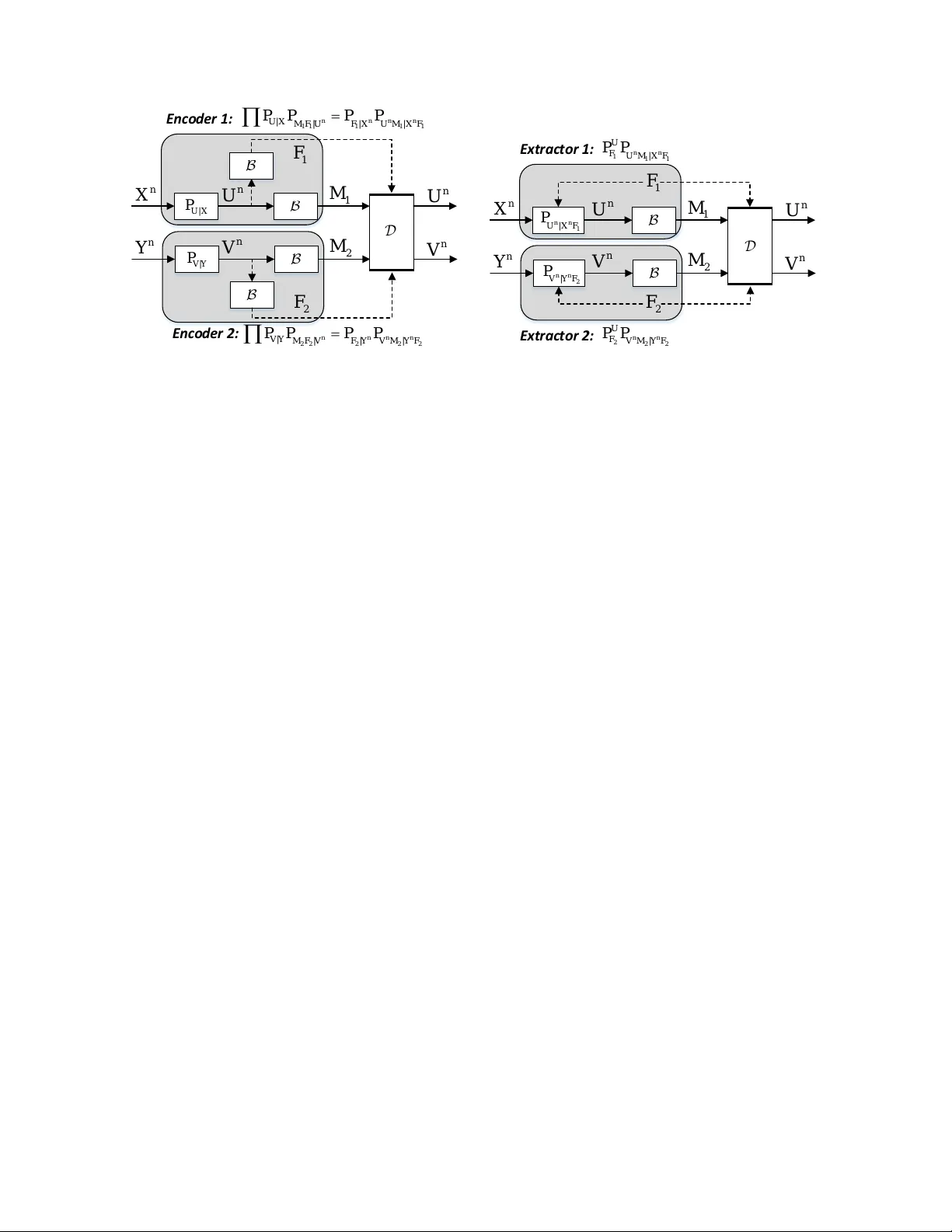
1 Generalized Common Informations: Measuring Commonness by the Conditional Maximal Correlation Lei Y u, Houqiang Li, Senior Member , IEEE , and Chang W en Chen, F ellow , IEEE Abstract In literature, different common informations were defined by G ´ acs and K ¨ orner , by W yner, and by K umar , Li, and Gamal, respectiv ely . In this paper, we define two generalized versions of common informations, named approximate and exact information-correlation functions , by exploiting the conditional maximal correlation as a commonness or priv acy measure. These two generalized common informations encompass the notions of G ´ acs-K ¨ orner’ s, W yner’ s, and Kumar-Li-Gamal’ s common informations as special cases. Furthermore, to gi ve operational characterizations of these two generalized common informations, we also study the problems of private sources synthesis and common information extraction, and sho w that the information-correlation functions are equal to the minimum rates of commonness needed to ensure that some conditional maximal correlation constraints are satisfied for the centralized setting versions of these problems. As a byproduct, the conditional maximal correlation has been studied as well. Index T erms Common information, conditional maximal correlation, information-correlation function, sources synthesis, infor- mation extraction I . I N T RO D U C T I O N Common information, as an information measure on the common part between two random variables, was first in vestigated by G ´ acs and K ¨ orner [ 1 ] in content of distributed common information e xtraction problem: extracting a same random v ariable from each of two sources individually . The common information of the sources is defined by the maximum information of the random v ariable that can be extracted from them. For correlated memoryless sources X , Y (taken from finite alphabets), [ 1 ] shows that the G ´ acs-K ¨ orner common information between them is C GK ( X ; Y ) = sup f ,g : f ( X )= g ( Y ) H ( f ( X )) . (1) Lei Y u is with the Department of Electrical and Computer Engineering, National Univ ersity of Singapore, Singapore (e-mail: leiyu@nus.edu.sg). This work was done when he w as at University of Science and T echnology of China. Houqiang Li is with the Department of Electronic Engineering and Information Science, University of Science and T echnology of China, Hefei, China (e-mail: lihq@ustc.edu.cn). Chang W en Chen is with Department of Computer Science and Engineering, State Univ ersity of New Y ork at Buffalo, Buf falo, NY , USA (e-mail: chencw@buf falo.edu). July 25, 2017 DRAFT It also can be e xpressed as C GK ( X ; Y ) = inf P U | X Y : C GK ( X ; Y | U )=0 I ( X Y ; U ) , (2) (the proof of ( 2 ) is giv en in Appendix A ), where C GK ( X ; Y | U ) := sup f ,g : f ( X,U )= g ( Y ,U ) H ( f ( X , U ) | U ) (3) denotes the conditional common information between X, Y gi ven U . The constraint C GK ( X ; Y | U ) = 0 in ( 2 ) implies all the common information between X , Y is contained in U . W yner [ 3 ] studied distrib uted source synthesis (or distributed source simulation) problem, and defined common information in a different w ay . Specifically , he defined common information as the minimum information rate needed to generate sources in a distributed manner with asymptotically vanishing normalized relative entropy between the induced distrib ution and some target joint distrib ution. Gi ven a target distribution P X Y , this common information is proven to be C W ( X ; Y ) = inf P U | X Y : X → U → Y I ( X Y ; U ) . (4) Furthermore, as a related problem, the problem of exactly generating target sources was studied by Kumar , Li, and Gamal recently [ 12 ]. The notion of e xact common information (rate) (denoted as K K LG ( X ; Y ) ) is introduced, which is defined to be the minimum code rate to ensure the induced distribution is exactly (instead approximately) same to some target joint distribution. By comparing these common informations, it is easy to show that C GK ( X ; Y ) ≤ I ( X ; Y ) ≤ C W ( X ; Y ) ≤ K K LG ( X ; Y ) ≤ H ( X Y ) . Observe that in the definitions of G ´ acs-K ¨ orner and W yner common informations, different dependency constraints are used. G ´ acs-K ¨ orner common information requires the common variable U to be some function of each of the sources (or equi valently , there is no conditional common information given U ); while W yner common information requires the sources conditionally independent giv en the common variable U . These two constraints are closely related to an important dependency measure, Hirscbfeld-Gebelein-Renyi maximal correlation (or simply maximal corr elation ). This correlation measures the maximum (Pearson) correlation between square integrable real-v alued random variables generated by the indi vidual random variables. According to the definition, maximal correlation is in variant on bijecti ve mappings (or robust to bijective transform), hence it reveals some kind of intrinsic dependency between two sources. This measure was first introduced by Hirschfeld [ 5 ] and Gebelein [ 4 ], then studied by R ´ enyi [ 6 ], and recently it has been exploited to some interesting problems of information theory , such as measure of non-local correlations [ 9 ], maximal correlation secrecy [ 10 ], con verse result of distributed communication [ 14 ], etc. Furthermore, maximal correlation also indicates the existence of G ´ acs-K ¨ orner or W yner common information: There exists G ´ acs-K ¨ orner common information between two sources if and only if the maximal correlation between them equals one; and there exists W yner common information between two sources if and only if the maximal correlation between them is positi ve. The common informations proposed by G ´ acs and K ¨ orner and by W yner (or by Kumar , Li, and Gamal) are defined in two dif ferent problems: distrib uted common information e xtraction and distributed source synthesis. In these problems, the common informations are defined from different points of vie w . One attempt to unify them can 2 be found in [ 11 ], where Kamath and Anantharam con verted common information extraction problem into a special case of distributed source synthesis problem by specifying the synthesized distribution to be that of the common randomness. In this paper, we attempt to giv e another unification of the existing common informations. Specifically , we unify and generalize the G ´ acs-K ¨ orner and W yner common informations by defining a generalized common information, (appr oximate) information-correlation function . In this generalized definition, the conditional maximal correlation (the conditional dependency of the sources given the common randomness) is exploited to measure the priv acy (or commonness), and the mutual information is used to measure the information amount of such common randomness. The G ´ acs-K ¨ orner common information and W yner common information are two special and extreme cases of our generalized definition with correlation respecti vely being 0 and 1 − 1 , and hence both of them can be seen as hard-measures of common information. Howe ver , in our definition, correlation could be any number between 0 and 1, hence our definition gi ves a soft-measure of common information. Our results give a more comprehensive answer to the classic problem: What is the common information between two correlated sources? Furthermore, similarly we also unify and generalize the G ´ acs-K ¨ orner and Kumar -Li-Gamal common informations into another generalized common information, (exact) information-correlation function . T o give an operational interpretation of the approximate and exact generalized common informations, we also study common information extraction problem and pri vate sources synthesis problem, and sho w that the information-correlation functions correspond to the minimum achie vable rates under pri vacy constraints for the centralized case of each problem. The rest of this paper is organized as follows. Section II summarizes definitions and properties of maximal correlation. Section III defines information-correlation function and pro vides the basic properties. Sections IV and V in vestigate the pri vate sources synthesis problem and common information extraction problem respectively . Finally , Section VI gi ves the concluding remarks. A. Notation and Preliminaries W e use P X ( x ) to denote the probability distribution of random variable X , which is also shortly denoted as P X or P ( x ) . W e also use P X and Q X to denote different probability distribution with common alphabet X . W e use P U X to denote the uniform distribution over the set X , unless otherwise stated. W e use f P or f Q to denote a quantity or operation f that is defined on pmf P or Q . The total v ariation distance between two probability measures P and Q with common alphabet is defined by k P − Q k T V := sup A ∈F | P ( A ) − Q ( A ) | (5) where F is the σ -algebra of the probability space. In this paper, some achie vability schemes inv olves a random codebook C (or a random binning B ). For simplicity , we also denote the induced conditional distribution P X |C = c (giv en C = c ) as P X (suppressing the condition C = c ), which can be seen as a random pmf . For any pmfs P X and Q X on X , we write P X  ≈ Q X if k P X − Q X k T V <  for non-random pmfs, or E C k P X − Q X k T V <  for random pmfs. For any two sequences of pmfs P X ( n ) and Q X ( n ) on X ( n ) (where X ( n ) is 1 1 − implies the correlation approaching 1 from the left. 3 arbitrary and it differs from X n which is a Cartesian product), we write P X ( n ) ≈ Q X ( n ) if lim n →∞ k P X ( n ) − Q X ( n ) k T V = 0 for non-random pmfs, or lim n →∞ E C k P X ( n ) − Q X ( n ) k T V = 0 for random pmfs. The following properties of total v ariation distance hold. Property 1. [ 19 ], [ 22 ] T otal variation distance satisfies: 1) If the support of P and Q is a countable set X , then k P − Q k T V = 1 2 X x ∈X | P ( x ) − Q ( x ) | . (6) 2) Let  > 0 and let f ( x ) be a function with bounded range of width b > 0 . Then P X  ≈ Q X ⇒ | E P f ( X ) − E Q f ( X ) | < b, (7) wher e E P indicates that the expectation is tak en with r espect to the distrib ution P . 3) P X ( n ) ≈ Q X ( n ) ⇒ P X ( n ) P Y ( n ) | X ( n ) ≈ Q X ( n ) P Y ( n ) | X ( n ) , P X ( n ) P Y ( n ) | X ( n ) ≈ Q X ( n ) Q Y ( n ) | X ( n ) ⇒ P X ( n ) ≈ Q X ( n ) . 4) F or any two sequences of non-r andom pmfs P X ( n ) Y ( n ) and Q X ( n ) Y ( n ) , if P X ( n ) P Y ( n ) | X ( n ) ≈ Q X ( n ) Q Y ( n ) | X ( n ) , then there exists a sequence x ( n ) ∈ X ( n ) such that P Y ( n ) | X ( n ) = x ( n ) ≈ Q Y ( n ) | X ( n ) = x ( n ) . 5) If P X ( n ) ≈ Q X ( n ) and P X ( n ) P Y ( n ) | X ( n ) ≈ P X ( n ) Q Y ( n ) | X ( n ) , then P X ( n ) P Y ( n ) | X ( n ) ≈ Q X ( n ) Q Y ( n ) | X ( n ) . I I . ( C O N D I T I O NA L ) M A X I M A L C O R R E L A T I O N In this section, we first define sev eral correlations, including (Pearson) correlation, correlation ratio, and maximal correlation, and then study their properties. These concepts and properties will be used to define and in vestigate information-correlation functions in subsequent sections. In this section, we assume all alphabets are general (not limited to finite or countable) unless otherwise stated. A. Definition Definition 1. For any random v ariables X and Y with alphabets X ⊆ R and Y ⊆ R , the (Pearson) correlation of X and Y is defined by ρ ( X ; Y ) =    cov ( X,Y ) √ var ( X ) √ var ( Y ) , if var ( X ) var ( Y ) > 0 , 0 , if var ( X ) var ( Y ) = 0 . (8) Moreov er , the conditional correlation of X and Y giv en another random v ariable U is defined by ρ ( X ; Y | U ) =    E [ cov ( X,Y | U )] √ E [ var ( X | U )] √ E [ var ( Y | U )] , if E [ var ( X | U )] E [ var ( Y | U )] > 0 , 0 , if E [ var ( X | U )] E [ var ( Y | U )] = 0 . (9) Definition 2. For any random variables X and Y with alphabets X ⊆ R and Y , the correlation ratio of X on Y is defined by θ ( X ; Y ) = sup g ρ ( X ; g ( Y )) , (10) 4 where the supremum is taken ov er all the functions g : Y 7→ R . Moreov er , the conditional correlation ratio of X on Y giv en another random v ariable U with alphabet U is defined by θ ( X ; Y | U ) = sup g ρ ( X ; g ( Y , U ) | U ) , (11) where the supremum is taken over all the functions g : Y × U 7→ R . Remark 1 . Note that in general θ ( X ; Y ) 6 = θ ( Y ; X ) and θ ( X ; Y | U ) 6 = θ ( Y ; X | U ) . Definition 3. For any random variables X and Y with alphabets X and Y , the maximal correlation of X and Y is defined by ρ m ( X ; Y ) = sup f ,g ρ ( f ( X ); g ( Y )) , (12) where the supremum is taken ov er all the functions f : X 7→ R , g : Y 7→ R . Moreov er , the conditional maximal correlation of X and Y giv en another random v ariable U with alphabet U is defined by ρ m ( X ; Y | U ) = sup f ,g ρ ( f ( X, U ); g ( Y , U ) | U ) , (13) where the supremum is taken over all the functions f : X × U 7→ R , g : Y × U 7→ R . It is easy to v erify that ρ m ( X ; Y | U ) = sup f θ ( f ( X , U ); Y | U ) . (14) Note that the unconditional versions of correlation coefficient, correlation ratio, and maximal correlation hav e been well studied in literature. The conditional versions are first introduced by Beigi and Gohari recently [ 9 ], where it is named as maximal corr elation of a box and used to study the problem of non-local correlations. In this paper , we will well study conditional maximal correlation (and conditional correlation ratio), and give some useful properties. B. Properties According to the definition, maximal correlation remains the same after applying bijecti ve transform (one-to-one correspondence) on each of the v ariables. Hence it is robust to bijective transform. Furthermore, for finite valued random v ariables maximal correlation ρ m ( X ; Y | U ) can be characterized by the second largest singular value λ 2 ( u ) of the matrix Q u with entries Q u ( x, y ) := p ( x, y | u ) p p ( x | u ) p ( y | u ) = p ( x, y , u ) p p ( x, u ) p ( y , u ) . (15) Lemma 1. (Singular value characterization). F or any random variables X , Y , U, ρ m ( X ; Y | U ) = sup u : P ( u ) > 0 λ 2 ( u ) . (16) Remark 2 . This shows the conditional maximal correlation is consistent with the unconditional version ( U = ∅ ) [ 2 ] ρ m ( X ; Y ) = λ 2 . (17) 5 Furthermore, for any random v ariables X , Y , U with finite alphabets, the supremum in ( 12 ), ( 13 ) and ( 16 ) is actually a maximum. The proof of this lemma is gi ven in Appendix B . This lemma giv es a simple approach to compute (conditional) maximal correlation. Observe that λ 2 ( u ) is equal to the maximal correlation ρ m ( X ; Y | U = u ) between X and Y under condition U = u , and under distribution P X Y | U = u . Hence Lemma 1 leads to the follo wing result. Lemma 2. (Alternative c haracterization). F or any r andom variables X, Y , U, ρ m ( X ; Y | U ) = sup u : P ( u ) > 0 ρ m ( X ; Y | U = u ) . (18) Note that the right-hand side of ( 18 ) was first defined by Beigi and Gohari [ 9 ]. This lemma implies the equiv alence between the conditional maximal correlation defined by us and that defined by Beigi and Gohari. Furthermore, Lemmas 1 and 2 also hold for continuous random variables, if the constraint of P ( u ) > 0 is replaced with p ( u ) > 0 . Here p ( u ) denotes the probability density function (pdf) of U . Notice that Lemmas 1 and 2 imply that ρ m ( X ; Y | U ) can be dif ferent for different distributions of X, Y , even if the distributions are only different up to a zero measure set. In measure theory , people usually do not care the difference with zero measure. Therefore, we refine the definition of conditional maximal correlation for continuous random variables by defining a robust version as follows. e ρ m ( X ; Y | U ) := inf q X Y U : q X Y U = p X Y U a.s. ρ m,q ( X ; Y | U ) , (19) for continuous random variables X, Y , U, with pdf p X Y U . W e name e ρ m ( X ; Y | U ) as r obust conditional maximal corr elation . Obviously , for discrete random variables case, robust conditional maximal correlation is consistent with conditional maximal correlation. Moreover , if we take inf q X Y U : q X Y U = p X Y U a.s. operation on each side of an equality or inequality about q X Y U , it usually does not change the equality or inequality . Hence in this paper, we only consider conditional maximal correlations rather than their robust versions. Lemma 3. (TV bound on maximal corr elation). F or any random variables X, Y , U with finite alphabets, ρ m,Q ( X ; Y | U ) ≥ ρ m,P ( X ; Y | U ) − 4 δ P m 1 + 4 δ P m , (20) wher e P m = min x,y ,u : P ( x,y ,u ) > 0 P ( x, y | u ) , and δ = max u : P ( u ) > 0 k P X Y | U = u − Q X Y | U = u k T V . Remark 3 . Lemma 3 implies ρ m,P ( X ; Y | U ) − 4 δ P m 1 + 4 δ P m ≤ ρ m,Q ( X ; Y | U ) ≤  1 + 4 δ Q m  ρ m,P ( X ; Y | U ) + 4 δ Q m , (21) where Q m = min x,y ,u : Q ( x,y,u ) > 0 Q ( x, y | u ) . Pr oof: Assume u achie ves the supremum in ( 18 ), and f , g satisfying E P [ f ( X, U ) | U = u ] = 0 , E P [ g ( Y , U ) | U = u ] = 0 , var P [ f ( X, U ) | U = u ] = 1 , var P [ g ( Y , U ) | U = u ] = 1 , achie ves ρ m,P ( X ; Y | U ) . Then P ( x | u ) f 2 ( x, u ) ≤ P x P ( x | u ) f 2 ( x, u ) = 1 for any x, u , i.e., | f ( x, u ) | ≤ 1 p P ( x | u ) (22) 6 for any x, u such that P ( x | u ) > 0 . Furthermore, for any x, u such that P ( x | u ) > 0 , we have P ( x | u ) ≥ P ( x, y | u ) ≥ P m . Hence ( 22 ) implies | f ( x, u ) | ≤ 1 √ P m . (23) Similarly , we hav e | g ( y, u ) | ≤ 1 √ P m . (24) According to Property ( 7 ), the following inequalities hold. | E Q [ f ( X, U ) g ( Y , U ) | U ] − E P [ f ( X, U ) g ( Y , U ) | U ] | ≤ 2 δ P m (25) | E Q [ f ( X, U ) | U ] | ≤ 2 √ P m k P X | U − Q X | U k T V ≤ 2 δ √ P m (26) | E Q [ g ( Y , U ) | U ] | ≤ 2 √ P m k P Y | U − Q Y | U k T V ≤ 2 δ √ P m (27) | E Q [ f 2 ( X, U ) | U ] − 1 | ≤ 2 δ P m (28) and | E Q [ g 2 ( Y , U ) | U ] − 1 | ≤ 2 δ P m . (29) Therefore, we ha ve ρ m,Q ( X ; Y | U = u ) ≥ E Q [ f ( X, U ) g ( Y , U ) | U ] − E Q [ f ( X, U ) | U ] E Q [ g ( Y , U ) | U ] q E Q [ f 2 ( X, U ) | U ] − E 2 Q [ f ( X, U ) | U ] q E Q [ g 2 ( Y , U ) | U ] − E 2 Q [ g ( Y , U ) | U ] (30) ≥ E Q [ f ( X, U ) g ( Y , U ) | U ] − 4 δ P m q E Q [ f 2 ( X, U ) | U ] − 4 δ P m q E Q [ g 2 ( Y , U ) | U ] − 4 δ P m (31) ≥ ρ m,P ( X ; Y | U = u ) − 4 δ P m q 1 + 4 δ P m q 1 + 4 δ P m (32) = ρ m,P ( X ; Y | U = u ) − 4 δ P m 1 + 4 δ P m . (33) Lemma 4. (Continuity and discontinuity). Assume X, Y , U have finite alphabets. Then given P U , ρ m ( X ; Y | U ) is continuous in P X Y | U . Given P X Y | U , ρ m ( X ; Y | U ) is continuous on { P U : P U ( u ) > 0 , ∀ u ∈ U } . But in gener al, ρ m ( X ; Y | U ) is discontinuous in P X Y U . Pr oof: ( 21 ) implies for gi ven P U , as max u : P ( u ) > 0 k P X Y | U = u − Q X Y | U = u k T V → 0 , ρ m,Q ( X ; Y | U ) → ρ m,P ( X ; Y | U ) . Hence for gi ven P U , ρ m,P ( X ; Y | U ) is continuous in P X Y | U . Furthermore, since given P X Y | U , ρ m ( X ; Y | U ) = sup u : P ( u ) > 0 λ 2 ( u ) , we ha ve for given P X Y | U , ρ m ( X ; Y | U ) is continuous on { P U : P U ( u ) > 0 , ∀ u ∈ U } . But it is worth noting that ρ m ( X ; Y | U ) may be discontinuous at P U such that P U ( u ) = 0 for some u ∈ U . Therefore, Q X Y U → P X Y U in total variation sense does not necessarily imply ρ m,Q ( X ; Y | U ) → ρ m ( X ; Y | U ) . That is, the conditional maximal correlation may be discontinuous in probability distribution P X Y U . Furthermore, some other properties hold. 7 Lemma 5. (Concavity). Given P X Y | U , ρ m ( X ; Y | U ) is concave in P U . Pr oof: Fix P X Y | U . Assume R U = λP U + (1 − λ ) Q U , λ ∈ (0 , 1) , then by Lemma 2 , we have ρ m,R ( X ; Y | U ) = sup u : R ( u ) > 0 ρ m ( X ; Y | U = u ) (34) = sup u : P ( u ) > 0 or Q ( u ) > 0 ρ m ( X ; Y | U = u ) (35) = max ( sup u : P ( u ) > 0 ρ m ( X ; Y | U = u ) , sup u : Q ( u ) > 0 ρ m ( X ; Y | U = u ) ) (36) = max { ρ m,P ( X ; Y | U ) , ρ m,Q ( X ; Y | U ) } . (37) Hence ρ m,R ( X ; Y | U ) ≥ λρ m,P ( X ; Y | U ) + (1 − λ ) ρ m,Q ( X ; Y | U ) , i.e., ρ m ( X ; Y | U ) is conca ve in P U . Lemma 6. F or any random variables X, Y , Z , U , the following inequalities hold. 0 ≤ | ρ ( X ; Y | U ) | ≤ θ ( X ; Y | U ) ≤ ρ m ( X ; Y | U ) ≤ 1 . (38) Mor eover , ρ m ( X ; Y | U ) = 0 if and only if X and Y ar e conditionally independent given U ; ρ m ( X ; Y | U ) = 1 if and only if X and Y have G ´ acs-K ¨ orner common information given U. Pr oof: | E [ cov ( X, Y | U )] | = | E [( X − E [ X | U ])( Y − E [ Y | U ])] | (39) ≤ p E [( X − E [ X | U ]) 2 ] E [( Y − E [ Y | U ]) 2 ] (40) = p E [ var ( X | U )] E [ var ( Y | U )] , (41) where ( 40 ) follo ws from the Cauchy-Schwarz inequality . Hence 0 ≤ | ρ ( X ; Y | U ) | ≤ 1 (42) which further implies 0 ≤ | ρ ( X ; Y | U ) | ≤ θ ( X ; Y | U ) ≤ ρ m ( X ; Y | U ) ≤ 1 (43) since both θ ( X ; Y | U ) and ρ m ( X ; Y | U ) are conditional correlations for some variables. If X and Y are conditionally independent gi ven U , then for any functions f and g , f ( X , U ) and g ( Y , U ) are also conditionally independent given U . This leads to ρ m ( X ; Y | U ) = 0 . Con versely , if ρ m ( X ; Y | U ) = 0 , then ρ ( f ( X, U ); g ( Y , U ) | U ) = 0 (44) for any functions f and g . For any x, u , set f ( X , U ) = 1 { X = x, U = u } and g ( Y , U ) = 1 { Y = y , U = u } , then E [ cov ( X, Y | U )] = P ( X = x, Y = y | U = u ) − P ( X = x | U = u ) P ( Y = y | U = u ) (45) 8 = P X Y | U ( x, y | u ) − P X | U ( x | u ) P Y | U ( y | u ) . (46) Hence ( 44 ) implies P X Y | U ( x, y | u ) = P X | U ( x | u ) P Y | U ( y | u ) . (47) This implies X and Y are conditionally independent gi ven U . Therefore, ρ m ( X ; Y | U ) = 0 if and only if X and Y are conditionally independent given U. Assume X and Y hav e G ´ acs-K ¨ orner common information given U , i.e., f ( X , U ) = g ( Y , U ) with probability 1 for some functions f and g such that H ( f ( X, U ) | U ) > 0 . Then E v ar ( f ( X , U ) | U ) E var ( g ( Y , U ) | U ) > 0 , and ρ m ( X ; Y | U ) ≥ ρ ( f ( X , U ); g ( Y , U ) | U ) ≥ 1 . (48) Combining this with ρ m ( X ; Y | U ) ≤ 1 , we ha ve ρ m ( X ; Y | U ) = 1 . Assume ρ m ( X ; Y | U ) = 1 , then f ( X , U ) = g ( Y , U ) with probability 1 for some functions f and g such that E var ( f ( X , U ) | U ) E var ( g ( Y , U ) | U ) > 0 , or equi valently , H ( f ( X , U ) | U ) > 0 . This implies X and Y have G ´ acs- K ¨ orner common information given U . Therefore, ρ m ( X ; Y | U ) = 1 if and only if X and Y have G ´ acs-K ¨ orner common information gi ven U . Lemma 7. F or any random variables X, Y , Z , U , the following pr operties hold. θ ( X ; Y Z | U ) ≥ θ ( X ; Y | U ); (49) ρ m ( X ; Y Z | U ) ≥ ρ m ( X ; Y | U ); (50) θ ( X ; Y | U ) = s E [ var ( E [ X | Y U ] | U )] E [ var ( X | U )] = s 1 − E [ var ( X | Y U )] E [ var ( X | U )] ; (51) ρ m ( X ; Y | U ) = sup f s E [ var ( E [ f ( X, U ) | Y U ] | U )] E [ var ( f ( X, U ) | U )] = sup f s 1 − E [ var ( f ( X, U ) | Y U )] E [ var ( f ( X, U ) | U )] . (52) In particular if U is deg enerate, then the inequalities above reduce to θ ( X ; Y Z ) ≥ θ ( X ; Y ); (53) ρ m ( X ; Y Z ) ≥ ρ m ( X ; Y ); (54) θ ( X ; Y ) = s var ( E [ X | Y ]) var ( X ) = s 1 − E [ var ( X | Y )] var ( X ) ; (55) 9 ρ m ( X ; Y ) = sup f s var ( E [ f ( X ) | Y ]) var ( f ( X )) = sup f s 1 − E [ var ( f ( X ) | Y )] var ( f ( X )) . (56) Remark 4 . Correlation ratio is also closely related to Minimum Mean Square Error (MMSE). The optimal MMSE estimator is E [ X | Y U ] , hence the variance of the MMSE for estimating X giv en ( Y , U ) is mmse ( X | Y U ) = E ( X − E [ X | Y U ]) 2 = E [ v ar ( X | Y U )] = E [ v ar ( X | U )](1 − θ 2 ( X ; Y | U )) . Pr oof: According to definitions of conditional correlation ratio and conditional maximal correlation, ( 49 ) and ( 50 ) can be proven easily . In fact, we may , without loss of the generality , consider only such function g for which E [ g ( Y , U ) | U = u ] = 0 , ∀ u and v ar ( g ( Y , U ) | U = u ) = 1 , ∀ u and suppose E [ X ] = 0 , E [ var ( X | U )] = 1; for this case we have by the Cauchy- Schwarz inequality E [ cov ( X, g ( Y , U ) | U )] = E [( X − E [ X | U ])( g ( Y , U ) − E [ g ( Y , U ) | U ])] (57) = E [ E [( X − E [ X | U ]) | Y U ]( g ( Y , U ) − E [ g ( Y , U ) | U ])] (58) = E [( E [ X | Y U ] − E [ X | U ])( g ( Y , U ) − E [ g ( Y , U ) | U ])] (59) ≤ p E [( E [ X | Y U ] − E [ X | U ]) 2 ] E [( g ( Y , U ) − E [ g ( Y , U ) | U ]) 2 ] (60) = p E [ var ( E [ X | Y U ] | U )] E [ var ( g ( Y , U ) | U )] . (61) Therefore, θ ( X ; Y | U ) = sup g E [ cov ( X, g ( Y , U ) | U )] p E [ var ( X | U )] E [ var ( g ( Y , U ) | U )] (62) ≤ s E [ var ( E [ X | Y U ] | U )] E [ var ( X | U )] . (63) It is easy to v erify that equality holds if and only if g ( Y , U ) = α E [ X | Y U ] for some constant α > 0 . Hence θ ( X ; Y | U ) = s E [ var ( E [ X | Y U ] | U )] E [ var ( X | U )] . (64) Furthermore, by la w of total variance var ( Y ) = E var ( Y | X ) + var ( E ( Y | X )) (65) and the conditional version E [ var ( X | U )] = E [ var ( X | Y U )] + E [ var ( E [ X | Y U ] | U )] , (66) we have θ ( X ; Y | U ) = s E [ var ( E [ X | Y U ] | U )] E [ var ( X | U )] = s 1 − E [ var ( X | Y U )] E [ var ( X | U )] . (67) 10 Furthermore, since ρ m ( X ; Y | U ) = sup f θ ( f ( X , U ); Y | U ) , ( 52 ) follo ws straightforwardly from ( 67 ). Lemma 8. (Correlation ratio equality). F or any r andom variables X, Y , U, 1 − θ 2 ( X ; Y Z | U ) = (1 − θ 2 ( X ; Z | U ))(1 − θ 2 ( X ; Y | Z U )); (68) 1 − ρ 2 m ( X ; Y Z | U ) ≥ (1 − ρ 2 m ( X ; Z | U ))(1 − ρ 2 m ( X ; Y | Z U )); (69) θ ( X ; Y Z | U ) ≥ θ ( X ; Y | Z U ); (70) ρ m ( X ; Y Z | U ) ≥ ρ m ( X ; Y | Z U ) . (71) Remark 5 . ( 71 ) is very similar to I ( X ; Y Z | U ) ≥ I ( X ; Y | Z U ) . Furthermore, ρ m ( X ; Y | U V ) ≥ ρ m ( X ; Y | U ) or ρ m ( X ; Y | U V ) ≤ ρ m ( X ; Y | U ) does not always hold. This is also similar to that I ( X ; Y | U V ) ≥ I ( X ; Y | U ) or I ( X ; Y | U V ) ≤ I ( X ; Y | U ) does not alw ays hold. Pr oof: From ( 51 ), we have 1 − θ 2 ( X ; Y Z | U ) = E [ var ( X | Y Z U )] E [ var ( X | U )] , (72) 1 − θ 2 ( X ; Z | U ) = E [ var ( X | Z U )] E [ var ( X | U )] , (73) and 1 − θ 2 ( X ; Y | Z U ) = E [ var ( X | Y Z U )] E [ var ( X | Z U )] . (74) Hence ( 68 ) follo ws immediately . Suppose f achieves ρ m ( X ; Y Z | U ) , i.e., the supremum in ( 13 ), then 1 − ρ 2 m ( X ; Y Z | U ) = 1 − θ 2 ( f ( X, U ); Y Z | U ) (75) = (1 − θ 2 ( f ( X, U ); Z | U ))(1 − θ 2 ( f ( X, U ); Y | Z U )) (76) ≥ (1 − ρ 2 m ( X ; Z | U ))(1 − ρ 2 m ( X ; Y | Z U )) . (77) Furthermore, θ 2 ( X ; Z | U ) ≥ 0 , hence ( 70 ) follo ws immediately from ( 68 ). Suppose f 0 achiev es ρ m ( X ; Y | Z U ) , then ρ m ( X ; Y | Z U ) = θ ( f 0 ( X, U ); Y | Z U ) ≤ θ ( f 0 ( X, U ); Y Z | U ) ≤ ρ m ( X ; Y Z | U ) . (78) Lemma 9. F or any P U X Y V such that U → X → Y and X → Y → V , we have ρ m ( U X ; V Y ) = max { ρ m ( X ; Y ) , ρ m ( U ; V | X Y ) } . (79) Remark 6 . A similar result can be found in [ 9 , Eqn. (4)], where Beigi and Gohari only pro ved the equality above as an inequality . Pr oof: Beigi and Gobari [ 9 , Eqn. (4)] have proven ρ m ( U X ; V Y ) ≤ max { ρ m ( X ; Y ) , ρ m ( U ; V | X Y ) } . Hence we only need to pro ve that ρ m ( U X ; V Y ) ≥ max { ρ m ( X ; Y ) , ρ m ( U ; V | X Y ) } . According to the definition, ρ m ( U X ; V Y ) ≥ 11 ρ m ( X ; Y ) is straightforward. From ( 71 ) of Lemma 8 , we have ρ m ( U X ; V Y ) ≥ ρ m ( U X ; V | Y ) ≥ ρ m ( U ; V | X Y ) . This completes the proof. W e also prove that conditioning reduces covariance gap as shown in the following lemma, the proof of which is giv en in Appendix C . Lemma 10. (Conditioning r educes covariance gap). F or any r andom variables X, Y , Z, U, p E var ( X | Z U ) E var ( Y | Z U ) − E cov ( X , Y | Z U ) ≤ p E var ( X | Z ) E var ( Y | Z ) − E cov ( X , Y | Z ) , (80) i. e., p (1 − θ 2 ( X ; U | Z ))(1 − θ 2 ( Y ; U | Z ))(1 − ρ ( X, Y | Z U )) ≤ 1 − ρ ( X, Y | Z ) . (81) In particular , if Z is de generate , then p E var ( X | U ) E var ( Y | U ) − E cov ( X, Y | U ) ≤ p var ( X ) var ( Y ) − cov ( X, Y ) , (82) i. e., p (1 − θ 2 ( X ; U ))(1 − θ 2 ( Y ; U ))(1 − ρ ( X , Y | U )) ≤ 1 − ρ ( X , Y ) . (83) Remark 7 . The following two inequalities follows immediately . p (1 − ρ 2 m ( X ; U | Z ))(1 − θ 2 ( Y ; U | Z ))(1 − θ ( X , Y | Z U )) ≤ 1 − θ ( X , Y | Z ) , (84) and p (1 − ρ 2 m ( X ; U | Z ))(1 − ρ 2 m ( Y ; U | Z ))(1 − ρ m ( X, Y | Z U )) ≤ 1 − ρ m ( X, Y | Z ) . (85) Furthermore, there are also some other remarkable properties. Lemma 11. (T ensorization). Assume given U, ( X n , Y n ) is a sequence of pairs of conditionally independent random variables, then we have ρ m ( X n ; Y n | U ) = sup 1 ≤ i ≤ n ρ m ( X i ; Y i | U ) . (86) Pr oof: The unconditional version ρ m ( X n ; Y n ) = sup 1 ≤ i ≤ n ρ m ( X i ; Y i ) , (87) for a sequence of pairs of independent random v ariables ( X n , Y n ) is proven in [ 2 , Thm. 1]. Using this result and Lemma 1 , we have ρ m ( X n ; Y n | U ) = sup u : P ( u ) > 0 ρ m ( X n ; Y n | U = u ) (88) = sup u : P ( u ) > 0 sup 1 ≤ i ≤ n ρ m ( X i ; Y i | U = u ) (89) = sup 1 ≤ i ≤ n sup u : P ( u ) > 0 ρ m ( X i ; Y i | U = u ) (90) = sup 1 ≤ i ≤ n ρ m ( X i ; Y i | U ) . (91) 12 Lemma 12. (Gaussian case). F or jointly Gaussian random variables X , Y , U , we have ρ m ( X ; Y ) = θ ( X ; Y ) = θ ( Y ; X ) = | ρ ( X ; Y ) | , (92) ρ m ( X ; Y | U ) = θ ( X ; Y | U ) = θ ( Y ; X | U ) = | ρ ( X ; Y | U ) | . (93) Pr oof: The unconditional version ( 92 ) is prov en in [ 13 , Sec. IV , Lem. 10.2]. On the other hand, gi ven U = u, ( X , Y ) also follows jointly Gaussian distribution, and ρ ( X ; Y | U = u ) = ρ ( X ; Y | U ) for different u . Hence ρ m ( X ; Y | U ) = sup u : P ( u ) > 0 ρ m ( X ; Y | U = u ) = sup u : P ( u ) > 0 | ρ ( X ; Y | U = u ) | = | ρ ( X ; Y | U ) | . Furthermore, both θ ( X ; Y | U ) and θ ( Y ; X | U ) are between ρ m ( X ; Y | U ) and | ρ ( X ; Y | U ) | . Hence ( 93 ) holds. Lemma 13. (Data pr ocessing inequality). If random variables X, Y , Z , U form a Markov chain X → ( Z, U ) → Y , then | ρ ( X ; Y | U ) | ≤ θ ( X ; Z | U ) θ ( Y ; Z | U ) , (94) θ ( X ; Y | U ) ≤ θ ( X ; Z | U ) ρ m ( Y ; Z | U ) , (95) ρ m ( X ; Y | U ) ≤ ρ m ( X ; Z | U ) ρ m ( Y ; Z | U ) . (96) Mor eover , the equalities hold in ( 94 ) - ( 96 ) , if ( X , Z, U ) and ( Y , Z , U ) have the same joint distribution. In particular if U is de generate , then | ρ ( X ; Y ) | ≤ θ ( X ; Z ) θ ( Y ; Z ) , (97) θ ( X ; Y ) ≤ θ ( X ; Z ) ρ m ( Y ; Z ) , (98) ρ m ( X ; Y ) ≤ ρ m ( X ; Z ) ρ m ( Y ; Z ) . (99) Pr oof: Consider that E [ cov ( X, Y | U )] = E [( X − E [ X | U ])( Y − E [ Y | U ])] (100) = E [ E [( X − E [ X | U ])( Y − E [ Y | U ]) | Z U ]] (101) = E [ E [ X − E [ X | U ] | Z U ] E [ Y − E [ Y | U ] | Z U ]] (102) = E [( E [ X | Z U ] − E [ X | U ])( E [ Y | Z U ] − E [ Y | U ])] (103) ≤ p E [( E [ X | Z U ] − E [ X | U ]) 2 ] E [( E [ Y | Z U ] − E [ Y | U ]) 2 ] (104) = p E [ var ( E [ X | Z U ] | U )] E [ var ( E [ Y | Z U ] | U )] (105) where ( 102 ) follo ws by conditional independence, and ( 104 ) follows the Cauchy-Schw arz inequality . Hence | ρ ( X ; Y | U ) | = E [ cov ( X, Y | U )] p E [ var ( X | U )] p E [ var ( Y | U )] (106) ≤ s E [ var ( E [ X | Z U ] | U )] E [ var ( E [ Y | Z U ] | U )] E [ var ( X | U )] E [ var ( Y | U )] (107) 13 = θ ( X ; Z | U ) θ ( Y ; Z | U ) . (108) It is easy to v erify the equalities hold if ( X, Z , U ) and ( Y , Z, U ) ha ve the same joint distribution. Similarly , ( 95 ) and ( 96 ) can be proven as well. Furthermore, correlation ratio and maximal correlation are also related to rate-distortion theory . Lemma 14. (Relationship to rate-distortion function) Let R X | U ( D ) denote the conditional rate distrib ution function for sour ce X given U with quadratic distortion measur e d ( x, ˆ x ) = ( x − ˆ x ) 2 . Then fr om rate-distortion theory , we have I ( X ; Y | U ) ≥ R X | U ( E [ var ( X | Y U )]) (109) = R X | U ( E [ var ( X | U )](1 − θ 2 ( X ; Y | U ))) (110) ≥ R X | U ( E [ var ( X | U )](1 − ρ 2 ( X ; Y | U ))) . (111) F r om Shannon lower bound, I ( X ; Y | U ) ≥ R X | U ( E [ var ( X | Y U )]) (112) ≥ h ( X | U ) − 1 2 log(2 π e E [ var ( X | U )](1 − θ 2 ( X ; Y | U ))) . (113) If ( X , U ) is jointly Gaussian, then I ( X ; Y | U ) ≥ 1 2 log + ( 1 1 − θ 2 ( X ; Y | U ) ) (114) ≥ 1 2 log + ( 1 1 − ρ 2 ( X ; Y | U ) ) . (115) In particular if U is deg enerate, then I ( X ; Y ) ≥ R X ( E [ var ( X | Y )]) (116) = R X ( var ( X )(1 − θ 2 ( X ; Y ))) . (117) F r om Shannon lower bound, I ( X ; Y ) ≥ R X ( E [ var ( X | Y )]) (118) ≥ h ( X ) − 1 2 log(2 π e (1 − θ 2 ( X ; Y ))) . (119) If X is Gaussian, then I ( X ; Y ) ≥ 1 2 log + ( 1 1 − θ 2 ( X ; Y ) ) (120) ≥ 1 2 log + ( 1 1 − ρ 2 ( X ; Y ) ) . (121) From the properties above, it can be observed that maximal correlation or correlation ratio has many similar properties as those of mutual information, such as in variance to one-to-one transform, chain rule (correlation ratio equality), data processing inequality , etc. On the other hand, maximal correlation or correlation ratio also has some different properties, such as for a sequence of pairs of independent random variables, the mutual information 14 between them is the sum of mutual information of all pairs of components (i.e., additivity); while the maximal correlation is the maximum one of the maximal correlations of all pairs of components (i.e., tensorization). C. Extension: Smooth Maximal Correlation Next we e xtend maximal correlation to smooth v ersion. Analogous extensions can be found in [ 15 ] and [ 16 ], where R ´ enyi div ergence and generalized Brascamp-Lieb-like (GBLL) rate are extended to the corresponding smooth versions. Definition 4. For any random variables X and Y with alphabets X ⊆ R and Y ⊆ R , and  ∈ (0 , 1) , the  -smooth (Pearson) correlation and the  -smooth conditional (Pearson) correlation of X and Y given another random v ariable U are respectively defined by e ρ  ( X ; Y ) := inf Q X Y : k Q X Y − P X Y k T V ≤  ρ Q ( X ; Y ) , (122) and e ρ  ( X ; Y | U ) := inf Q X Y U : k Q X Y U − P X Y U k T V ≤  ρ Q ( X ; Y | U ) . (123) Definition 5. For any random v ariables X and Y with alphabets X ⊆ R and Y , and  ∈ (0 , 1) , the  -smooth correlation ratio and the  -smooth conditional correlation ratio of X and Y giv en another random v ariable U are respectiv ely defined by e θ  ( X ; Y ) := inf Q X Y : k Q X Y − P X Y k T V ≤  θ Q ( X ; Y ) , (124) and e θ  ( X ; Y | U ) := inf Q X Y U : k Q X Y U − P X Y U k T V ≤  θ Q ( X ; Y | U ) . (125) Definition 6. For an y random v ariables X and Y with alphabets X and Y , and  ∈ (0 , 1) , the  -smooth maximal correlation and the  -smooth conditional maximal correlation of X and Y gi ven another random variable U are respectiv ely defined by e ρ  m ( X ; Y ) := inf Q X Y : k Q X Y − P X Y k T V ≤  ρ m,Q ( X ; Y ) , (126) and e ρ  m ( X ; Y | U ) := inf Q X Y U : k Q X Y U − P X Y U k T V ≤  ρ m,Q ( X ; Y | U ) . (127) According to definition, obviously we ha ve e ρ  ( X ; Y | U ) ≤ ρ ( X ; Y | U ) , (128) e θ  ( X ; Y | U ) ≤ θ ( X ; Y | U ) , (129) e ρ  m ( X ; Y | U ) ≤ ρ m ( X ; Y | U ) . (130) Furthermore, note that adding inf Q X Y U : k Q X Y U − P X Y U k T V ≤  operation before both sides of an equality or inequality about P X Y U does not change the equality or inequality . Hence some of above lemmas still hold for  -smooth version, e.g., Lemmas 1 , 2 , 6 , and 7 , and also ( 70 ) and ( 71 ) of Lemma 8 . 15 I I I . G E N E R A L I Z E D C O M M O N I N F O R M A T I O N : I N F O R M A T I O N - C O R R E L A T I O N F U N C T I O N In this section, we generalize the existing common informations, and define β -approximate common information (or approximate information-correlation function) and β -e xact common information (or e xact information-correlation function), which measure how much information are approximately or exactly β -correlated between two variables. Different from the existing common informations, β -common information is a function of conditional maximal correlation β ∈ [0 , 1] , and hence it provides a soft-measure of common information. As in the previous section, in this section we also assume all alphabets are general unless otherwise stated. A. Definition Suppose U is a common random v ariable extracted from X, Y , satisfying priv acy constraint ρ m ( X ; Y | U ) ≤ β , then the β -priv ate information corresponding to U should be H ( X Y | U ) . W e define the β -priv ate information as the maximum of such pri v ate informations o ver all possible U . Definition 7. For sources X , Y , and β ∈ [0 , 1] , the β -approximate priv ate information of X and Y is defined by B β ( X ; Y ) = sup P U | X Y : ρ m ( X ; Y | U ) ≤ β H ( X Y | U ) . (131) Common information is defined as C β ( X ; Y ) = H ( X Y ) − B β ( X ; Y ) , which is equiv alent to the following definition. Definition 8. For sources X, Y , and β ∈ [0 , 1] , the β -approximate common information (or approximate information- correlation function) of X and Y is defined by C β ( X ; Y ) = inf P U | X Y : ρ m ( X ; Y | U ) ≤ β I ( X Y ; U ) . (132) Similarly , e xact common information can be generalized to β -exact common information as well. Definition 9. For sources X, Y , and β ∈ [0 , 1] , the β -exact common information (rate) (or exact information- correlation function) of X and Y is defined by K β ( X ; Y ) = lim n →∞ inf P U n | X n Y n : ρ m ( X n ; Y n | U n ) ≤ β 1 n H ( U n ) . (133) Furthermore, for β ∈ (0 , 1] , we also define C β − ( X ; Y ) = lim α ↑ β C α ( X ; Y ) , (134) K β − ( X ; Y ) = lim α ↑ β K α ( X ; Y ) . (135) B. Properties These two generalized common informations have the follo wing properties. Lemma 15. (a) F or the infimum in ( 132 ) , it suf fices to consider the variable U with alphabet |U | ≤ |X ||Y | + 1 . 16 (b) F or any random variables X, Y , C β ( X ; Y ) and K β ( X ; Y ) are decreasing in β . Mor eover , C β ( X ; Y ) ≤ K β ( X ; Y ) , for 0 ≤ β ≤ 1 , (136) C β ( X ; Y ) = K β ( X ; Y ) = 0 , for ρ m ( X ; Y ) ≤ β ≤ 1 , (137) C 0 ( X ; Y ) = C W ( X ; Y ) , (138) K 0 ( X ; Y ) = K K LG ( X ; Y ) , (139) C 1 − ( X ; Y ) = K 1 − ( X ; Y ) = C GK ( X ; Y ) , (140) wher e K K LG ( X ; Y ) := lim n →∞ inf P U n | X n Y n : X n → U n → Y n 1 n H ( U n ) denotes the exact common information (r ate) pr oposed by K umar , Li, and Gamal [ 12 ]. (c) If P U | X,Y achie ves the infimum in ( 132 ) , then ρ m ( X ; Y | U ) ≤ ρ m ( X ; Y | V ) for any V such that X Y → U → V . Remark 8 . For any random variables X , Y , C β ( X ; Y ) is decreasing in β , but it is not necessarily con ve x or concav e; see the Gaussian source case in the next subsection. C β ( X ; Y ) and K β ( X ; Y ) are discontinuous at β = 1 , if there is common information between the sources. Lemma 15 implies G ´ acs-K ¨ orner common information, W yner common information and exact common information are extreme cases of β -approximate common information or β -exact common information. Pr oof: T o show (a), we only need to sho w for any variable U , there always e xists another variable U 0 such that |U 0 | ≤ |X ||Y | + 1 , ρ m ( X ; Y | U 0 ) = ρ m ( X ; Y | U ) , and I ( X Y ; U 0 ) = I ( X Y ; U ) . Suppose ρ m ( X ; Y | U = u ∗ ) = ρ m ( X ; Y | U ) . According to Support Lemma [ 7 ], there e xists a random v ariable U 0 with U 0 ⊆ U and |U 0 | ≤ |X ||Y | + 1 such that P U 0 ( u ∗ ) = P U ( u ∗ ) , (141) H ( X Y | U 0 ) = H ( X Y | U ) , (142) P X Y = X u 0 P U 0 P X Y | U 0 . (143) ( 141 ) implies ρ m ( X ; Y | U 0 ) = ρ m ( X ; Y | U ) . ( 143 ) implies H ( X Y ) is also preserved, and hence I ( X Y ; U ) = I ( X Y ; U 0 ) . This completes the proof of (a). (b) ( 136 ) and ( 137 ) follow straightforwardly from the definitions. According to the definitions and Lemma 6 ( ρ m ( X ; Y | U ) = 0 if and only if X → U → Y ), we can easily obtain ( 138 ) and ( 139 ). Next we prove ( 140 ). Consider C 1 − ( X ; Y ) = inf P U | X,Y : ρ m ( X ; Y | U ) < 1 I ( X Y ; U ) . (144) Assume G ´ acs-K ¨ orner common information is f GK ( X, Y ) . Set U = f GK ( X, Y ) , then we ha ve ρ m ( X ; Y | U ) < 1 , (145) I ( X Y ; U ) = H ( f GK ( X, Y )) = C GK ( X ; Y ) . (146) 17 3   ; W C I XY W    | H X W   | HYW   H X Y 1 1   ; C I X Y U   2 2   = GK C H V   ; I X Y   | H Y X   | H X Y Fig. 1. Illustration of the relationship among joint entrop y , mutual information, W yner common information, generalized common information, and GK common information, where W , V and U are the W yner , GK, and ρ -correlated common randomnesses, respecti v ely , and Re gion 1 represents H ( X Y | U ) and Re gion 2 represents H ( X Y | V ) . The inequalities C GK ≤ I ( X ; Y ) ≤ C W and C GK = C 0 ≤ C ρ ≤ lim ρ ↑ 1 C ρ = C W , ∀ 0 ≤ ρ < 1 hold. The total v ariation distance between tw o probability measures P and Q with common alphabet is defined by k P − Q k T V , sup A ∈F | P ( A ) − Q ( A ) | , (1) where F is the σ -algebra of the probability space. The follo wing properties of total v ariation distance hold. Pr operty 1. [ 13 ] T otal variation distance satisfies: 1) If the support of P and Q is a countable set X , then k P − Q k T V = 1 2 X x ∈X | P ( { x } ) − Q ( { x } ) | . (2) 2) Let  > 0 and let f ( x ) be a function with bounded r ang e of width b > 0 . Then k P − Q k T V <  = ⇒   E P f ( X ) − E Q f ( X )   < b, (3) wher e E P indicates that the e xpectation is tak en with r espect to the distrib ution P . 3) Let P X P Y | X and Q X P Y | X be two joint distrib utions with common c hannel P Y | X . Then k P X P Y | X − Q X P Y | X k T V = k P X − Q X k T V . (4) I I . M A X I M A L C O R R E L A T I O N In this section, we define se v eral correlations, including correlation coef ficient, correlation ratio, and maximal correlation, and then study their properties. Definition 1. F or an y random v ariables X and Y with alphabets X ⊆ R and Y ⊆ R , the (Pearson) correlation of X and Y is defined by ρ ( X ; Y ) =      co v ( X ,Y ) √ v ar ( X ) √ v ar ( Y ) , if v ar ( X ) v ar ( Y ) > 0 , 0 , if v ar ( X ) v ar ( Y ) = 0 . (5) September 19, 2016 DRAFT Fig. 1. Illustration of the relationship among joint entropy , mutual information, W yner common information, generalized common information, and G ´ acs-K ¨ orner common information, where W, V and U are the W yner, G ´ acs-K ¨ orner , and β -common random variables, respectively , and Region 1 represents H ( X Y | U ) and Region 2 represents H ( X Y | V ) . These terms satisfy C GK ≤ I ( X ; Y ) ≤ C W and C GK = C 0 ≤ C β ≤ C 1 − ( X ; Y ) = C W , ∀ 0 ≤ β < 1 . Hence by definition, C 1 − ( X ; Y ) ≤ C GK ( X ; Y ) . (147) On the other hand, for any U such that ρ m ( X ; Y | U ) < 1 , the G ´ acs-K ¨ orner common information is determined by U , i.e., f GK ( X, Y ) = g ( U ) for some function g . Therefore, we hav e I ( X Y ; U ) = I ( X Y ; U, f GK ( X, Y )) ≥ H ( f GK ( X, Y )) = C GK ( X ; Y ) . (148) Hence C 1 − ( X ; Y ) ≥ C GK ( X ; Y ) . (149) Combining ( 147 ) and ( 149 ) gi ves us C 1 − ( X ; Y ) = C GK ( X ; Y ) . (150) Similarly K 1 − ( X ; Y ) = C GK ( X ; Y ) can be proven as well. (c) Suppose P U | X ,Y achiev es the infimum in ( 132 ). If V satisfies both X Y → U → V and X Y → V → U , the we have ρ m ( X ; Y | U ) = ρ m ( X ; Y | U V ) = ρ m ( X ; Y | V ) . If V satisfies X Y → U → V but does not satisfy X Y → V → U , then I ( X Y ; U ) = I ( X Y ; U V ) > I ( X Y ; V ) . Hence ρ m ( X ; Y | U ) ≤ ρ m ( X ; Y | V ) , otherwise it contradicts with that P U | X ,Y achiev es the infimum in ( 132 ). Fig. 1 illustrates the relationship among joint entropy , mutual information, G ´ acs-K ¨ orner common information, W yner common information, and generalized common information. Lemma 16. (Additivity and subadditivity). Assume ( X i , Y i ) n i =1 is a sequence of pairs of independent random variables, then we have C β ( X n ; Y n ) = n X i =1 C β ( X i ; Y i ) , (151) and K β ( X i ; Y i ) ≤ K β ( X n ; Y n ) ≤ n X i =1 K β ( X i ; Y i ) . (152) 18 Pr oof: F or ( 151 ) it suf fices to pro ve the n = 2 case, i.e., C β ( X 2 ; Y 2 ) = C β ( X 1 ; Y 1 ) + C β ( X 2 ; Y 2 ) . (153) Observe for any P U | X 2 Y 2 , ρ m ( X 2 ; Y 2 | U ) ≥ ρ m ( X i ; Y i | U ) , i = 1 , 2 , (154) and I ( X 2 Y 2 ; U ) ≥ I ( X 1 Y 1 ; U ) + I ( X 2 Y 2 ; U | X 1 Y 1 ) (155) = I ( X 1 Y 1 ; U ) + I ( X 2 Y 2 ; U X 1 Y 1 ) (156) ≥ I ( X 1 Y 1 ; U ) + I ( X 2 Y 2 ; U ) . (157) Hence we ha ve C β ( X 2 ; Y 2 ) ≥ C β ( X 1 ; Y 1 ) + C β ( X 2 ; Y 2 ) . (158) Moreov er , if we choose P U | X 2 Y 2 = P ∗ U 1 | X 1 Y 1 P ∗ U 2 | X 2 Y 2 in C β ( X 2 ; Y 2 ) , where P ∗ U i | X i Y i , i = 1 , 2 , is the distribu- tion achieving C β ( X i ; Y i ) , then we have ρ m ( X 2 ; Y 2 | U ) = max i ∈{ 1 , 2 } ρ m ( X i ; Y i | U i ) ≤ β , (159) and I ( X 2 Y 2 ; U ) = I ( X 1 Y 1 ; U 1 ) + I ( X 2 Y 2 ; U 2 ) = C β ( X 1 ; Y 1 ) + C β ( X 2 ; Y 2 ) . (160) Therefore, C β ( X 2 ; Y 2 ) = inf P U | X 2 Y 2 : ρ m ( X 2 ; Y 2 | U ) ≤ β I ( X 2 Y 2 ; U ) ≤ C β ( X 1 ; Y 1 ) + C β ( X 2 ; Y 2 ) . (161) ( 158 ) and ( 161 ) implies ( 151 ) holds for n = 2 . Furthermore, the first inequality of ( 152 ) can be obtained directly from the definition of K β . The second inequality of ( 152 ) can be obtained by restricting P U | X n Y n to the one with independent components (similar as the proof of ( 161 )). For continuous sources, a lower bound on approximate common information is gi ven in the following theorem. Theorem 1. (Lower bound on C β ( X ; Y ) ). F or any continuous sour ces ( X , Y ) with correlation coefficient β 0 , we have C β ( X ; Y ) ≥ h ( X Y ) − 1 2 log  (2 π e (1 − β 0 )) 2 1 + β 1 − β  (162) for 0 ≤ β ≤ β 0 , and C β ( X ; Y ) = 0 for β 0 ≤ β ≤ 1 . Pr oof: I ( X Y ; U ) = h ( X Y ) − h ( X Y | U ) (163) ≥ h ( X Y ) − E U 1 2 log  (2 π e ) 2 det(Σ X Y | U )  (164) ≥ h ( X Y ) − 1 2 log  (2 π e ) 2 det( E U Σ X Y | U )  (165) 19 0 0.2 0.4 0.6 0.8 1 0 0.5 1 1.5 2 C β β Fig. 2. Information-correlation function for Gaussian sources in Theorem 2 with β 0 = 0 . 9 . = h ( X Y ) − 1 2 log  (2 π e ) 2  E var ( X | U ) E var ( Y | U ) − ( E co v ( X , Y | U )) 2  (166) = h ( X Y ) − 1 2 log  (2 π e ) 2 E var ( X | U ) E var ( Y | U )(1 − ρ 2 ( X ; Y | U ))  (167) ≥ h ( X Y ) − 1 2 log  (2 π e ) 2 ( 1 − β 0 1 − ρ ( X , Y | U ) ) 2 (1 − ρ 2 ( X ; Y | U ))  (168) = h ( X Y ) − 1 2 log  (2 π e (1 − β 0 )) 2 1 + ρ ( X ; Y | U ) 1 − ρ ( X ; Y | U )  (169) ≥ h ( X Y ) − 1 2 log  (2 π e (1 − β 0 )) 2 1 + β 1 − β  , (170) where ( 165 ) follows from the function log (det( · )) is concave on the set of symmetric positiv e definite square matrices [ 8 , p.73], ( 168 ) follo ws from Lemma 10 , and ( 170 ) follows from ρ ( X ; Y | U ) ≤ β . (171) The equality holds in Theorem 1 if X, Y are jointly Gaussian. The proof is gi ven in Appendix D . Theorem 2. (Gaussian sources). F or jointly Gaussian sour ces X , Y with corr elation coef ficient β 0 , C ( G ) β ( X ; Y ) = 1 2 log +  1 + β 0 1 − β 0 / 1 + β 1 − β  . (172) Remark 9 . Specialized to the W yner common information, C ( G ) W ( X ; Y ) = C ( G ) 0 ( X ; Y ) = 1 2 log +  1 + β 0 1 − β 0  , which was first given in [ 21 ]. For the doubly symmetric binary source, an upper bound on common information is given in the following theorem. 20 Theorem 3. (Doubly symmetric binary sour ce (DSBS)). F or doubly symmetric binary sour ce ( X , Y ) with cr ossover pr obability p 0 , i.e., P X Y =   1 2 (1 − p 0 ) 1 2 p 0 1 2 p 0 1 2 (1 − p 0 )   , we have C ( B ) β ( X ; Y ) ≤ 1 + H 2 ( p 0 ) − H 4 1 2 1 − p 0 + s 1 − 2 p 0 − β 1 − β ! , 1 2 1 − p 0 − s 1 − 2 p 0 − β 1 − β ! , p 0 2 , p 0 2 ! (173) for 0 ≤ β < 1 − 2 p 0 , and C ( B ) β ( X ; Y ) = 0 for β ≥ 1 − 2 p 0 , wher e H 2 and H 4 denote the binary and quaternary entr opy functions, r espectively , i.e., H 2 ( p ) = − p log p − (1 − p ) log(1 − p ) , (174) H 4 ( a, b, c, d ) = − a log a − b log b − c log c − d log d. (175) Pr oof: Assume p is a v alue such that 2 p ¯ p = p 0 , ¯ p := 1 − p . Then ( X , Y ) can be e xpressed as X = U ⊕ V ⊕ Z 1 , (176) Y = U ⊕ V ⊕ Z 2 , (177) where U ∼ Bern ( 1 2 ) , V ∼ Bern ( α ) with 0 ≤ α ≤ 1 , Z 1 ∼ Bern ( p ) , and Z 2 ∼ Bern ( p ) are independent. Hence we hav e P V ⊕ Z 1 ,V ⊕ Z 2 =   a p ¯ p p ¯ p b   with a = αp 2 + ¯ α ¯ p 2 , b = α ¯ p 2 + ¯ αp 2 , and ρ m ( X, Y | U ) = ρ m ( V ⊕ Z 1 , V ⊕ Z 2 ) . (178) By using the formula ρ 2 m ( X, Y ) ≤ " X x,y P 2 ( x, y ) P ( x ) P ( y ) # − 1 (179) for ( X , Y ) with at least one of them being binary-v alued, we hav e ρ m ( X, Y ) = 1 − 2 p 0 . (180) Hence C ( B ) β ( X ; Y ) = 0 for β ≥ 1 − 2 p 0 . Next we consider the case β ≤ 1 − 2 p 0 . (181) T o guarantee ρ m ( V ⊕ Z 1 , V ⊕ Z 2 ) ≤ β , we choose a = 1 2 1 − p 0 + s 1 − 2 p 0 − β 1 − β ! (182) b = 1 2 1 − p 0 − s 1 − 2 p 0 − β 1 − β ! . (183) This leads to the inequality ( 335 ). This completes the proof. 21 C. Relationship to Rate-Distortion Function The approximate information-correlation function can be rewritten as C β ( X ; Y ) = inf P U | X,Y : d ( P U X Y ) ≤ β I ( X Y ; U ) . (184) where d ( P U X Y ) := ρ m ( X ; Y | U ) . This e xpression has a form similar to rate-distortion function, if we consider maximal correlation as a special “distortion measure”. But it is worth nothing that maximal correlation is taken on the distribution of X , Y , instead of on them itself. Information-correlation function is also related to the rate-pri vacy function [ 20 ] g β ( X ; Y ) := sup P U | Y : ρ m ( X ; U ) ≤ β I ( Y ; U ) , (185) in which U can be thought of as the extracted information from Y under priv acy constraint ρ m ( X ; U ) ≤ β . But there are three differences between g β ( X ; Y ) and C β ( X ; Y ) . 1) The priv acy constraint in g β ( X ; Y ) is a constraint on unconditional maximal correlation, and moreov er , this unconditional maximal correlation is that between the remote source X and extracted information U , instead of between the sources. Hence g β ( X ; Y ) is not symmetric respect to X, Y . 2) In g β ( X ; Y ) , U is extracted from Y instead of both X , Y , hence X → Y → U is restricted in g β ( X ; Y ) . 3) The optimization in C β ( X ; Y ) is infimum, while in g β ( X ; Y ) is supremum. I V . P R I V A T E S O U R C E S S Y N T H E S I S In order to provide an operational interpretation for information-correlation functions C β ( X ; Y ) and K β ( X ; Y ) , in this section, we consider private sources synthesis pr oblem . W e sho w that the information-correlation functions correspond to the minimum achie v able rates for the centralized setting version of this problem. A. Problem Setup Consider priv ate sources synthesis problem sho wn in Fig. 3 , where a simulator generates two source sequences X n and Y n from a common random variable M . X n and Y n are restricted to follow i.i.d. according to a tar get distribution Y P X Y . Definition 10. A generator is defined by a pmf P M and a stochastic mapping P X n Y n | M : M 7→ X n × Y n . Furthermore, Shannon’ s zero-error source coding theorem states that, it is possible to compress a message M (using a variable length coding) at rate R for suf ficiently lar ge n if R > 1 n H ( M ) ; and con versely , it is possible only if R ≥ 1 n H ( M ) . Hence we define the achiev ability of tuple ( R, β ) as follo ws. Definition 11. The tuple ( R, β ) is approximately or exactly achiev able if there exists a sequence of generators such that 1) rate constraint: lim sup n →∞ 1 n H ( M ) ≤ R ; (186) 2) priv acy constraint: ρ m ( X n ; Y n | M ) ≤ β , ∀ n ; (187) 22 19 G e n e r a t o r n X n Y M ∈ G e ne r a t or 1 n X n Y [ 2 ] nR M  G e ne r a t or 2 [ 2 ] nR M  Fig. 3. Pri v ate source synthesis probl em: 1) pri v ac y constraint ρ m ( X n ; Y n | M ) ≤ ρ ; 2) source dist rib ution constraint lim n →∞ k P X n Y n − Q X n Y n k T V = 0 in weak sense, or P X n Y n = Q X n Y n in strong sense. 2) approximate sources distrib ution constraint: lim n →∞    P X n Y n − Y P X Y    T V = 0 , (150) or e xact sources distrib ution constraint: P X n Y n = Y P X Y . (151) Definition 35. The rate-correlation functi on for approximate pri v ate source synthesis is defined by R S S ( ρ ) , inf { R : ( R , ρ ) is achie v able } . Similarly , the rate-correlati on function for e xact pri v ate source synthesis is defined by R ( E ) S S ( ρ ) , inf { R : ( R , ρ ) is achie v able } . Besides, we also consider distrib uted setting as sho wn in Fig. 3(b) . F or this case, the source synthesis problem is named distrib uted pri v ate source synthesis. Definition 36. An ( n, R ) distrib uted generator is defined by tw o stochastic mappings: P X n | M :  2 nR  7→ X n and P Y n | M :  2 nR  7→ Y n . Definition 37. The tuple ( R , ρ ) is approximately or e xactly achie v able for distrib uted setting if there e xists a sequence of ( n, R ) distrib uted generators such that 1) pri v ac y constraint: ( 149 ); 2) approximate source distrib ution constraint: ( 150 ), or e xact source distrib ution constraint: ( 151 ). Definition 38. The rate-correlation function for distrib uted approximate pri v ate or e xact source synthesis is defi ned by R D S S ( ρ ) , inf { R : ( R , ρ ) is achie v able } and R ( E ) D S S ( ρ ) , inf { R : ( R , ρ ) is achie v able } , respecti v ely . Then for distrib uted setting, pri v ac y constraint ρ m ( X n ; Y n | M ) = 0 (152) is satisfied immediately . Therefore, September 19, 2016 DRAFT 19 G e n e r a t o r n X n Y [ 2 ] nR M  G e ne r a t or 1 n X n Y M ∈ G e ne r a t or 2 M ∈ Fig. 3. Pri v ate source synthesis probl em: 1) pri v ac y constraint ρ m ( X n ; Y n | M ) ≤ ρ ; 2) source dist rib ution constraint lim n →∞ k P X n Y n − Q X n Y n k T V = 0 in weak sense, or P X n Y n = Q X n Y n in strong sense. 2) approximate sources distrib ution constraint: lim n →∞    P X n Y n − Y P X Y    T V = 0 , (150) or e xact sources distrib ution constraint: P X n Y n = Y P X Y . (151) Definition 35. The rate-correlation functi on for approximate pri v ate source synthesis is defined by R S S ( ρ ) , inf { R : ( R , ρ ) is achie v able } . Similarly , the rate-correlati on function for e xact pri v ate source synthesis is defined by R ( E ) S S ( ρ ) , inf { R : ( R , ρ ) is achie v able } . Besides, we also consider distrib uted setting as sho wn in Fig. 3(b) . F or this case, the source synthesis problem is named distrib uted pri v ate source synthesis. Definition 36. An ( n, R ) distrib uted generator is defined by tw o stochastic mappings: P X n | M :  2 nR  7→ X n and P Y n | M :  2 nR  7→ Y n . Definition 37. The tuple ( R , ρ ) is approximately or e xactly achie v able for distrib uted setting if there e xists a sequence of ( n, R ) distrib uted generators such that 1) pri v ac y constraint: ( 149 ); 2) approximate source distrib ution constraint: ( 150 ), or e xact source distrib ution constraint: ( 151 ). Definition 38. The rate-correlation function for distrib uted approximate pri v ate or e xact source synthesis is defi ned by R D S S ( ρ ) , inf { R : ( R , ρ ) is achie v able } and R ( E ) D S S ( ρ ) , inf { R : ( R , ρ ) is achie v able } , respecti v ely . Then for distrib uted setting, pri v ac y constraint ρ m ( X n ; Y n | M ) = 0 (152) is satisfied immediately . Therefore, September 19, 2016 DRAFT Fig. 3. Priv ate source synthesis problem: (left) centralized setting; (right) distributed setting. In this problem we assume 1) rate constraint lim sup n →∞ 1 n H ( M ) ≤ R ; 2) priv acy constraint ρ m ( X n ; Y n | M ) ≤ β ; 3) source distribution constraint lim n →∞ k P X n Y n − Q X n Y n k T V = 0 in approximate synthesis sense, or P X n Y n = Q X n Y n in exact synthesis sense. For distributed setting, the M in the constraints is replaced with M 1 M 2 . 3) approximate sources distribution constraint: lim n →∞ k P X n Y n − Y P X Y k T V = 0 , (188) or exact sources distrib ution constraint: P X n Y n = Y P X Y , ∀ n. (189) Definition 12. The rate-correlation function for approximate priv ate sources synthesis is defined by R P S S ( β ) := inf { R : ( R , β ) is approximately achie vable } . Similarly , the rate-correlation function for exact priv ate sources syn- thesis is defined by R ( E ) P S S ( β ) := inf { R : ( R , β ) is e xactly achie vable } . Furthermore, we also consider distributed setting, which is shown in Fig. 3 (b). For this case, the source synthesis problem is named distributed private sour ces synthesis . Definition 13. A distrib uted generator is defined by a pmf P M and two stochastic mappings: P X n | M : M 7→ X n and P Y n | M : M 7→ Y n . Definition 14. The tuple ( R, β ) is approximately or exactly achiev able for distributed setting if there exists a sequence of distrib uted generators such that 1) rate constraint: ( 186 ); 2) priv acy constraint: ( 187 ); 3) approximate source distribution constraint: ( 188 ), or exact source distribution constraint: ( 189 ). Definition 15. The rate-correlation function for distributed approximate or exact priv ate sources synthesis is defined by R DP S S ( β ) := inf { R : ( R, β ) is approximately achiev able } and R ( E ) DP S S ( β ) := inf { R : ( R , β ) is e xactly achie vable } , respectiv ely . For distributed setting, pri v acy constraint ρ m ( X n ; Y n | M ) = 0 (190) 23 is satisfied immediately . Therefore, R DP S S ( β ) = R DP S S (0) , (191) R ( E ) DP S S ( β ) = R ( E ) DP S S (0) . (192) W e assume the synthesized sources ha ve finite alphabets. B. Main Result 1) Centralized Setting: For approximate pri vate sources synthesis, we have the follo wing theorems. The proof of Theorem 4 is gi ven in Appendix E . Theorem 4. F or appr oximate private sour ces synthesis, R P S S ( β ) = C β ( X ; Y ) . (193) Remark 10 . From the proof we can see that using fixed-length coding is suf ficient to achie ve the rate-correlation function R P S S ( β ) . Theorem 5. F or e xact private sour ces synthesis, R ( E ) P S S ( β ) = K β ( X ; Y ) . (194) Pr oof: Ac hievability: Suppose R > K β ( X ; Y ) . W e will show that the rate R is achiev able. Input Pr ocess Generator: Generate input source M according to pmf P U n . Source Generator: Upon m , the generator generate sources ( X n , Y n ) according to P X n Y n | U n ( x n , y n | m ) . For such generator , the induced ov erall distribution is P X n Y n M ( x n , y n , m ) := P X n Y n U n ( x n , y n , m ) . (195) This means ρ m ( X n ; Y n | M ) ≤ β , (196) since ρ m ( X n ; Y n | U n ) ≤ β . (197) Since K β ( X ; Y ) = lim n →∞ 1 n H ( U n ) for some U n , R ≥ 1 n ( H ( U n ) + 1) for n lar ge enough. By the achiev ability part of Shannon’ s zero-error source coding theorem, it is possible to exactly generate ( X n , Y n ) at rate at most 1 n ( H ( U n ) + 1) . Hence rate R is achie vable and thus R ( E ) P S S ( β ) ≤ K β ( X ; Y ) . Con verse: Now suppose a rate R is achiev able. Then there exists an ( n, R ) -generator that exactly generates ( X n , Y n ) such that ρ m ( X n ; Y n | M ) ≤ β . (198) By the con verse for Shannon’ s zero-error source coding theorem, lim n →∞ 1 n H ( M ) ≤ R. (199) 24 Therefore, R ≥ lim n →∞ 1 n H ( M ) ≥ lim n →∞ inf P U n | X n Y n : ρ m ( X n ,Y n | U n ) ≤ β 1 n H ( U n ) = K β ( X ; Y ) . (200) That is R ( E ) P S S ( β ) ≥ K β ( X ; Y ) . (201) 2) Distributed Setting: For distributed priv ate sources synthesis, we ha ve similar results. Theorem 6. F or distrib uted appr oximate private sour ces synthesis, R DP S S ( β ) = C 0 ( X ; Y ) . (202) Remark 11 . From the proof we can see that similar to centralized case, using fixed-length coding is also sufficient to achiev e the rate-correlation function R DP S S ( β ) for distrib uted case. Pr oof: The theorem was essentially same to W yner’ s result [ 3 ]. In the follo wing, we prove this theorem by following similar steps to the proof of the centralized case. Achie vability: Consider the generator used for the centralized case (see Appendix E-A ). Similar to the centralized case, we can prove if R > C 0 ( X ; Y ) , lim n →∞ E C k P X n Y n − Q X n Y n k T V = 0 . (203) Owing to the distributed setting, Mark ov chain X n → M → Y n holds. By Lemma 6 , we hav e ρ m ( X n ; Y n | M ) = 0 . (204) Hence R DP S S ( β ) ≤ C 0 ( X ; Y ) . (205) Con verse: By slightly modified the proof of centralized case and combining with Markov chain X n → M → Y n , we can sho w that R DP S S ( β ) ≥ C 0 ( X ; Y ) . (206) Theorem 7. F or distrib uted exact private sources synthesis, R ( E ) DP S S ( β ) = K 0 ( X ; Y ) . (207) Pr oof: Ac hievability: Suppose R > K 0 ( X ; Y ) . W e will show that the rate R is achiev able. Input Pr ocess Generator: Generate input source M according to P U n . Source Generator: Upon m , the generator 1 generates source X n according to P X n | U n ( x n | m ) , and the generator 2 generates source Y n according to P Y n | U n ( y n | m ) . 25 Similar to the centralized case, since ρ m ( X n ; Y n | U n ) = 0 , i.e., X n → U n → Y n , the induced overall distribution is P X n Y n M ( x n , y n , m ) := P U n ( m ) P X n | U n ( x n | m ) P Y n | U n ( y n | m ) = P X n Y n U n ( x n , y n , m ) . (208) This means P X n Y n ( x n , y n ) = n Y i =1 P X Y ( x i , y i ) . (209) and ρ m ( X n ; Y n | M ) = 0 ≤ β . (210) Hence the rate R is achiev able, which further implies R ( E ) DP S S ( β ) ≤ K 0 ( X ; Y ) . (211) Con verse: Suppose a rate R is achiev able. Then there exists an ( n, R ) -generator that exactly generates ( X n , Y n ) such that ρ m ( X n ; Y n | M ) ≤ β . (212) Owing to the distributed setting, Mark ov chain X n → M → Y n holds naturally . By Lemma 6 , we ha ve ρ m ( X n ; Y n | M ) = 0 . (213) Furthermore, by the conv erse for Shannon’ s zero-error source coding theorem, lim n →∞ 1 n H ( M ) ≤ R. (214) Therefore, R ≥ lim n →∞ 1 n H ( M ) ≥ lim n →∞ inf P U n | X n Y n : ρ m ( X n ,Y n | U n ) ≤ β 1 n H ( U n ) = K 0 ( X ; Y ) . (215) That is R ( E ) DP S S ( β ) ≥ K 0 ( X ; Y ) . (216) V . C O M M O N I N F O R M A T I O N E X T R A C T I O N In this section, we study another problem, common information extraction pr oblem , which provides another operational interpretation for information-correlation functions C β ( X ; Y ) and K β ( X ; Y ) . Similar to priv ate sources synthesis problem, the information-correlation functions are prov en to be the minimum achiev able rates for the centralized setting v ersion of this problem as well. 26 23 E x t r a c t o r n X n Y M ∈ E xt r a c t or 1 n X n Y 1 [ 2 ] nR M  E xt r a c t or 2 2 [ 2 ] nR M  Fig. 4. Common information e xtraction problem: (a) centralized setting; (b) distrib uted setting. 1) criterion 1 inf Q X , Y , M : k Q X n ,Y n ,M − P X n ,Y n ,M k T V → 0 lim sup n →∞ ρ m ( X n ; Y n | M ) ≤ ρ ; 2) ρ m ( X n ; Y n | M ) ≤ ρ. . The e xtractor e xtracts common information to satisfy the pri v ac y constraint measured by conditional maximal correlation. Definition 44. The tuple ( R , ρ ) is achie v able if there e xists a sequence of ( n, R ) e xtractors such that criterion 1: weak pri v ac y constraint inf Q X , Y , M : k Q X n ,Y n ,M − P X n ,Y n ,M k T V → 0 lim sup n →∞ ρ m ( X n ; Y n | M , Q X n ,Y n ,M ) ≤ ρ, (179) criterion 2: strong pri v ac y constraint ρ m ( X n ; Y n | M ) ≤ ρ. (180) Definition 45. The rate-correlation functions for weakly common infor mation e xtraction problem and strongly common information e xtraction problem are defined by R C I E ( ρ ) , inf { R : ( R , ρ ) is achie v able } and R ( E ) C I E ( ρ ) , inf { R : ( R , ρ ) is achie v able } , respecti v ely . Besides, we also consider distrib uted common information e xtraction. Definition 46. An ( n, R ) distrib uted e xtractor is defined by tw o stochastic mappings: P M 1 | X n : X n 7→  2 nR 1  and P M 2 | Y n : Y n 7→  2 nR 2  such that 1 n H ( M 1 M 2 ) ≤ R (181) for some R 1 , R 2 . Definition 47. The tuple ( R , ρ ) is achie v able for distrib uted setting if there e xists a sequence of ( n, R ) distrib uted e xtractors such that criterion 1 inf Q X , Y , M 1 , M 2 : k Q X n ,Y n ,M 1 ,M 2 − P X n ,Y n ,M 1 ,M 2 k T V → 0 lim sup n →∞ ρ m ( X n ; Y n | M 1 , M 2 , Q X n ,Y n ,M 1 ,M 2 ) ≤ ρ, (182) criterion 2 ρ m ( X n ; Y n | M 1 , M 2 ) ≤ ρ. (183) September 19, 2016 DRAFT 23 E x t r a c t o r n X n Y [ 2 ] nR M  E xt r a c t or 1 n X n Y 1 M ∈ E xt r a c t or 2 2 M ∈ Fig. 4. Common information e xtraction problem: (a) centralized setting; (b) distrib uted setting. 1) criterion 1 inf Q X , Y , M : k Q X n ,Y n ,M − P X n ,Y n ,M k T V → 0 lim sup n →∞ ρ m ( X n ; Y n | M ) ≤ ρ ; 2) ρ m ( X n ; Y n | M ) ≤ ρ. . The e xtractor e xtracts common information to satisfy the pri v ac y constraint measured by conditional maximal correlation. Definition 44. The tuple ( R , ρ ) is achie v able if there e xists a sequence of ( n, R ) e xtractors such that criterion 1: weak pri v ac y constraint inf Q X , Y , M : k Q X n ,Y n ,M − P X n ,Y n ,M k T V → 0 lim sup n →∞ ρ m ( X n ; Y n | M , Q X n ,Y n ,M ) ≤ ρ, (179) criterion 2: strong pri v ac y constraint ρ m ( X n ; Y n | M ) ≤ ρ. (180) Definition 45. The rate-correlation functions for weakly common infor mation e xtraction problem and strongly common information e xtraction problem are defined by R C I E ( ρ ) , inf { R : ( R , ρ ) is achie v able } and R ( E ) C I E ( ρ ) , inf { R : ( R , ρ ) is achie v able } , respecti v ely . Besides, we also consider distrib uted common information e xtraction. Definition 46. An ( n, R ) distrib uted e xtractor is defined by tw o stochastic mappings: P M 1 | X n : X n 7→  2 nR 1  and P M 2 | Y n : Y n 7→  2 nR 2  such that 1 n H ( M 1 M 2 ) ≤ R (181) for some R 1 , R 2 . Definition 47. The tuple ( R , ρ ) is achie v able for distrib uted setting if there e xists a sequence of ( n, R ) distrib uted e xtractors such that criterion 1 inf Q X , Y , M 1 , M 2 : k Q X n ,Y n ,M 1 ,M 2 − P X n ,Y n ,M 1 ,M 2 k T V → 0 lim sup n →∞ ρ m ( X n ; Y n | M 1 , M 2 , Q X n ,Y n ,M 1 ,M 2 ) ≤ ρ, (182) criterion 2 ρ m ( X n ; Y n | M 1 , M 2 ) ≤ ρ. (183) September 19, 2016 DRAFT Fig. 4. Common information extraction problem: (left) centralized setting; (right) distributed setting. In this problem we assume 1) rate constraint lim sup n →∞ 1 n H ( M ) ≤ R ; 2) weak pri vacy constraint: for any  > 0 , e ρ  m ( X n ; Y n | M ) ≤ β , ∀ n, or strong priv acy constraint: ρ m ( X n ; Y n | M ) ≤ β , ∀ n. For distributed setting, the variable M in the constraints is replaced with M 1 M 2 . A. Problem Setup As a counterpart of priv ate sources synthesis problem, we consider common information extraction problem shown in Fig. 4 , where an extractor extracts common random v ariable M from two source sequences X n and Y n . X n and Y n are i.i.d. according to P X Y . Definition 16. An e xtractor is defined by a stochastic mapping: P M | X n Y n : X n × Y n 7→ M . The extractor should extract an enough mount of common information to satisfy the priv acy constraint measured by conditional maximal correlation. Definition 17. The tuple ( R, β ) is weakly or strongly achie vable if there exists a sequence of extractors such that 1) rate constraint: lim sup n →∞ 1 n H ( M ) ≤ R ; (217) 2a) weak pri vacy constraint: for any  > 0 , it holds that e ρ  m ( X n ; Y n | M ) ≤ β , ∀ n, (218) where e ρ  m ( X n ; Y n | M ) denotes  -smooth conditional maximal correlation; see ( 127 ); 2b) or strong priv acy constraint: ρ m ( X n ; Y n | M ) ≤ β , ∀ n. (219) Common information corresponds to the smallest information rate that makes the privac y constraint satisfied, hence the common information indeed represents a kind of “core” information. Now we define the rate-correlation functions as follo ws. Definition 18. The rate-correlation functions for weakly and strongly common information extraction problems are defined by R C I E ( β ) := inf { R : ( R , β ) is weakly achiev able } and R ( E ) C I E ( β ) := inf { R : ( R , β ) is strongly achiev able } , respectiv ely . Furthermore, we also consider distrib uted common information extraction. 27 Definition 19. A distrib uted e xtractor is defined by tw o stochastic mappings P M 1 | X n : X n 7→ M 1 and P M 2 | Y n : Y n 7→ M 2 . Definition 20. The tuple ( R, β ) is achiev able for distributed setting if there e xists a sequence of distrib uted extractors such that 1) rate constraint: ( 217 ); 2a) weak pri vacy constraint: for any  > 0 , it holds that e ρ  m ( X n ; Y n | M 1 , M 2 ) ≤ β , ∀ n, (220) 2b) or strong priv acy constraint: ρ m ( X n ; Y n | M 1 , M 2 ) ≤ β , ∀ n. (221) Definition 21. The rate-correlation functions for distributed weakly and strongly common information extrac- tion problems are defined by R DC I E ( β ) := inf { R : ( R, β ) is weakly achiev able } and R ( E ) DC I E ( β ) := inf { R : ( R, β ) is strongly achiev able } , respectively . W e also assume the sources ha ve finite alphabets. B. Main Result 1) Centralized Setting: For weakly common information extraction, we have the following theorems. The proof of Theorem 8 is gi ven in Appendix F . Theorem 8. F or weakly common information e xtraction, R C I E ( β ) = C β ( X ; Y ) . (222) Remark 12 . From the proof we can see that using fixed-length coding is suf ficient to achie ve the rate-correlation function R C I E ( β ) . Theorem 9. F or str ongly common information e xtraction, R ( E ) C I E ( β ) = K β ( X ; Y ) . (223) Pr oof: Ac hievability: Suppose R > K β ( X ; Y ) . W e will show that the rate R is achiev able. Extractor: Upon ( x n , y n ) , the e xtractor generates m according to P U n | X n Y n ( m | x n , y n ) . For such extractor , the induced overall distribution is P X n Y n M ( x n , y n , m ) = P X n Y n U n ( x n , y n , m ) . (224) Hence ρ m ( X n ; Y n | M ) = ρ m ( X n ; Y n | U n ) ≤ β . (225) 28 Since K β ( X ; Y ) = lim n →∞ 1 n H ( U n ) , R ≥ 1 n ( H ( U n ) + 1) for n large enough. By the achiev ability part of Shannon’ s zero-error source coding theorem, it is possible to exactly generate ( X n , Y n ) at rate at most 1 n ( H ( U n ) + 1) . Hence rate R is achiev able and thus R ( E ) C I E ( β ) ≤ K β ( X ; Y ) . Con verse: Now suppose a rate R is achiev able. Then there exists a sequence of extractors that generate M such that ρ m ( X n ; Y n | M ) ≤ β , ∀ n. (226) By the con verse for Shannon’ s zero-error source coding theorem, lim n →∞ 1 n H ( M ) ≤ R. (227) Therefore, R ≥ lim n →∞ 1 n H ( M ) ≥ lim n →∞ inf P U n | X n Y n : ρ m ( X n ,Y n | U n ) ≤ β 1 n H ( U n ) = K β ( X ; Y ) . (228) That is R ( E ) C I E ( β ) ≥ K β ( X ; Y ) . (229) 2) Distributed Setting: For distributed common information extraction, we ha ve similar results. The follo wing theorems hold for weakly and strongly common information extraction, respectiv ely . The proof of Theorem 10 is giv en in Appendix G . Theorem 10. F or distrib uted weakly common information e xtraction, C ( D,LB ) β ( X ; Y ) ≤ R DC I E ( β ) = C ( D ) β ( X ; Y ) ≤ C ( D,U B ) β ( X ; Y ) , (230) wher e C ( D,U B ) β ( X ; Y ) := inf P U | X P V | Y : ρ m ( X,Y | U V ) ≤ β I ( X Y ; U V ) , (231) C ( D ) β ( X ; Y ) := lim n →∞ inf P U | X n P V | Y n : ρ m ( X n ; Y n | U V ) ≤ β 1 n I ( X n Y n ; U V ) , (232) C ( D,LB ) β ( X ; Y ) := inf P T P U V | X Y T : U T → X → Y ,X → Y → V T , ρ m ( U X ; V Y | T ) ≤ ρ m ( X ; Y ) , ρ m ( X,Y | U V T ) ≤ β I ( X Y ; U V | T ) . (233) Remark 13 . From the proof we can see that similar to centralized case, using fixed-length coding is also sufficient to achiev e the rate-correlation function R DC I E ( β ) for distrib uted case. Theorem 11. F or distrib uted str ongly common information extr action, R ( E ) DC I E ( β ) = K ( D ) β ( X ; Y ) , (234) wher e K ( D ) β ( X n ; Y n ) := lim n →∞ inf P U n | X n P V n | Y n : ρ m ( X n ,Y n | U n V n ) ≤ β 1 n H ( U n V n ) . (235) Pr oof: Ac hievability: Suppose R > K ( D ) β ( X ; Y ) . W e will show that the rate R is achiev able. 29 Extractor: Upon ( x n , Y n ) , the extractor 1 generates m 1 according to P U n | X n ( m 1 | x n ) , and extractor 2 generates m 2 according to P V n | Y n ( m 2 | y n ) . For such extractor , the induced overall distribution is P X n Y n M 1 M 2 ( x n , Y n , m 1 , m 2 ) = P X n Y n U n V n ( x n , Y n , m 1 , m 2 ) . (236) Hence ρ m ( X n ; Y n | M 1 M 2 ) = ρ m ( X n ; Y n | U n V n ) ≤ β . (237) Since G β ( X ; Y ) = lim n →∞ 1 n H ( U n V n ) , R ≥ 1 n ( H ( U n V n ) + 1) for n large enough. By the achiev ability part of Shan- non’ s zero-error source coding theorem, it is possible to e xactly generate ( X n , Y n ) at rate at most 1 n ( H ( U n V n ) + 1) . Hence rate R is achiev able and thus R ( E ) DC I E ( β ) ≤ K ( D ) β ( X ; Y ) . Con verse: Now suppose a rate R is achiev able. Then there exists a sequence of extractors that generate ( M 1 , M 2 ) such that ρ m ( X n ; Y n | M 1 M 2 ) ≤ β , ∀ n. (238) By the con verse for Shannon’ s zero-error source coding theorem, lim n →∞ 1 n H ( M 1 M 2 ) ≤ R. (239) Therefore, R ≥ lim n →∞ 1 n H ( M 1 M 2 ) ≥ lim n →∞ inf p U n | X n p V n | Y n : ρ m ( X n ,Y n | U n V n ) ≤ β 1 n H ( U n V n ) = K ( D ) β ( X ; Y ) . (240) That is R ( E ) DC I E ( β ) ≥ K ( D ) β ( X ; Y ) . (241) V I . C O N C L U D I N G R E M A R K S In this paper , we unify and generalize G ´ acs-K ¨ orner and W yner common informations, and define a generalized version of common information, (approximate) information-correlation function, by exploiting maximal correlation as a commonness or priv acy measure. The G ´ acs-K ¨ orner common information and W yner common information are two special and extreme cases of our generalized definition. Furthermore, similarly exact information-correlation function has been defined as well, which is a generalization of G ´ acs-K ¨ orner common information and Kumar - Li-Gamal common information. W e study the problems of common information extraction and priv ate sources synthesis, and show that these two information-correlation functions are equal to the optimal rates under giv en correlation constraints in the centralized cases of these problems. Our results ha ve a sequence of applications: • Dependency measure: The generalized common informations defined by us provide a fresh look at dependency . The more common information the sources share, the more dependent they are. T o normalize the (approximate) information-correlation function, we can define Γ β ( X ; Y ) = C β ( X ; Y ) H ( X , Y ) , (242) 30 or Γ β ( X ; Y ) = 1 − 2 − 2 C β ( X ; Y ) . (243) Furthermore, we define corr elation-information function as the in verse function of information-correlation function, i.e., β C ( X ; Y ) = inf P U | X Y : I ( X Y ; U ) ≤ C ρ m ( X ; Y | U ) , (244) which represents the source dependency after extracting C -rate common information from X , Y . Obviously β C ( X ; Y ) = ρ m ( X ; Y ) when C = 0 . Dependency measure can be further applied to feature extraction and image classification. Furthermore, conditional maximal correlation can be also applied to measure the dependency of distributed sources, which has been exploited to derive some conv erse results of distributed communication; see our another work [ 14 ]. • Game theory and correlation based secrecy: The common information e xtraction can be equi valently trans- formed into a zero-sum game problem. Consider two adversarial parties. One is Player A, and another one is Players B and C. Players A and B share a source X , and Players A and C share another source Y . Sources X , Y are correlated and memoryless. Players B and C cooperate to maximize the conditional correlation ρ ( f ( X n , M ); g ( Y n , M ) | M ) (or ρ Q ( f ( X n , M ); g ( Y n , M ) | M ) for some distribution Q X n Y n M ) ov er all functions f , g , where M is a message received from Player A through a rate-limited channel, and f ( X n , M ) and g ( Y n , M ) are the outputs of Players B and C respectiv ely . Player A generates M from X n , Y n and wants to minimize the optimal correlation induced by Players B and C (assume Player A does not know the distribution Q Players A and B choose). Then our result on common information extraction can directly apply to this case, and it implies the exact (or approximate) information-correlation function is equal to the minimum rate needed for Player A to force B and C’ s optimal strategy satisfying sup f ,g ρ ( f ( X n , M ); g ( Y n , M ) | M ) ≤ β (or inf k Q X n Y n M − P X n Y n M k T V ≤  sup f ,g ρ Q ( f ( X n , M ); g ( Y n , M ) | M ) ≤ β for any  > 0 ). • Priv acy protection in data collection or data mining: In data collection or data mining, priv acy protection of users’ data is an important problem. T o that end, we need first identify which part is common information and which part is priv ate information. Our result giv es a better answer to this question and hence it can be directly applied to pri vacy protection in data collection or data mining. • Priv acy constrained source simulation: As stated in [ 11 ], the pri vate sources simulation problem has natural applications in numerous areas – from game-theoretic coordination in a network to control of a dynamical system ov er a distributed network with priv acy protection. Our results are expected to be exploited in many future remote-controlled applications, such as drone-based delivery system, priv acy-preserving na vigation, secure network service, etc. A P P E N D I X A P RO O F O F E Q UA T I O N ( 2 ) First we pro ve inf P U | X Y : C GK ( X ; Y | U )=0 I ( X Y ; U ) ≤ C GK ( X ; Y ) . Assume f ∗ , g ∗ achiev e the supremum in ( 1 ), then we claim that setting U = f ∗ ( X ) = g ∗ ( Y ) , it holds that C GK ( X ; Y | U ) = 0 . W e use contradiction to 31 prov e this claim. Suppose C GK ( X ; Y | U ) > 0 , i.e., there exists a pair of f 0 , g 0 such that f 0 ( X, U ) = g 0 ( Y , U ) and H ( f 0 ( X, U ) | U ) > 0 . Since U is a function of X and also a function of Y , we can express f 0 ( X, U ) as f 00 ( X ) and g 0 ( Y , U ) as g 00 ( Y ) for some functions f 00 and g 00 . Setting f ( X ) = ( f ∗ ( X ) , f 00 ( X )) and g ( Y ) = ( g ∗ ( Y ) , g 00 ( Y )) , we have f ( X ) = g ( Y ) and H ( f ( X )) = H ( U ) + H ( f 0 ( X, U ) | U ) > H ( U ) . (245) This contradicts with the assumption of f ∗ , g ∗ achieving the supremum in ( 1 ). Therefore, C GK ( X ; Y | U ) = 0 . This implies inf P U | X Y : C GK ( X ; Y | U )=0 I ( X Y ; U ) ≤ H ( U ) = C GK ( X ; Y ) . (246) Next we prove inf P U | X Y : C GK ( X ; Y | U )=0 I ( X Y ; U ) ≥ C GK ( X ; Y ) . W e also assume f ∗ , g ∗ achiev e the supremum in ( 1 ). Then we claim that for any U such that C GK ( X ; Y | U ) = 0 , it holds that f ∗ ( X ) = g ∗ ( Y ) = κ ( U ) for some function κ , i.e., U contains the common randomness of X , Y . Next we prove this claim. Assume f 0 , g 0 achiev e the supremum in ( 3 ). Then we have C GK ( X ; Y | U ) = 0 implies H ( f 0 ( X, U ) | U ) = 0 , which further implies f 0 ( X, U ) is a function of U ; see [ 17 , Problem 2.5]. Setting f ( X , U ) = ( f ∗ ( X ) , f 0 ( X, U )) and g ( Y , U ) = ( g ∗ ( Y ) , g 0 ( Y , U )) , we hav e f ( X, U ) = g ( Y , U ) and H ( f 0 ( X, U ) | U ) ≤ H ( f ( X , U ) | U ) . (247) Owing to the optimality of f 0 , g 0 , the equality in ( 247 ) should hold. Therefore, H ( f ∗ ( X ) | U, f 0 ( X, U )) = 0 . This implies f ∗ ( X ) is a function of U and f 0 ( X, U ) . Combining it with that f 0 ( X, U ) is a function of U , we have f ∗ ( X ) is a function of U . Therefore, f ∗ ( X ) = g ∗ ( Y ) = κ ( U ) for some function κ . Using the claim, we ha ve inf P U | X Y : C GK ( X ; Y | U )=0 I ( X Y ; U ) ≥ inf P U | X Y : C GK ( X ; Y | U )=0 I ( X Y ; κ ( U )) (248) = inf P U | X Y : C GK ( X ; Y | U )=0 I ( X Y ; f ∗ ( X )) (249) = H ( f ∗ ( X )) (250) = C GK ( X ; Y ) . (251) Combining these tw o cases abo ve, we have inf P U | X Y : C GK ( X ; Y | U )=0 I ( X Y ; U ) = C GK ( X ; Y ) . A P P E N D I X B P RO O F O F L E M M A 1 A proof for the unconditional version of the lemma can be found in [ 23 ]. Here we extend the proof to the conditional v ersion. T o that end, we only consider finite valued random variables. For countably infinitely valued or continuous random variables, the result can be prov en similarly . 32 For finite valued random v ariables, we will show maximal correlation ρ m ( X ; Y | U ) can also be characterized by the second largest singular value of the matrix Q u with entries Q u ( x, y ) := p ( x, y | u ) p p ( x | u ) p ( y | u ) = p ( x, y , u ) p p ( x, u ) p ( y , u ) . W ithout loss of generality , we can re write ρ m ( X ; Y | U ) = sup f ,g E [ f ( X, U ) g ( Y , U )] , (252) where the maximization is tak en o ver all f , g such that E [ f ( X , U )] = E [ g ( Y , U )] = 0 , E v ar ( f ( X , U )) = E var ( g ( Y , U )) = 1 . Observe that E [ f ( X, U ) g ( Y , U )] = X x,y ,u ( f ( x, u ) p p ( x, u )) Q u ( x, y )( g ( y, u ) p p ( y , u )) , (253) X x p p ( x, u ) Q u ( x, y ) = p p ( y , u ) , X y Q u ( x, y ) p p ( y , u ) = p p ( x, u ) , (254) and the conditions E [ f ( X , U )] = 0 and E [ g ( Y , U )] = 0 are respectively equi valent to requiring that ( x, u ) 7→ f ( x, u ) p p ( x, u ) is orthogonal to ( x, u ) 7→ p p ( x, u ) and that ( y , u ) 7→ g ( y, u ) p p ( y , u ) is orthogonal to ( y , u ) 7→ p p ( y , u ) . By Singular V alue Decomposition, Q u = n X i =1 λ u,i a u,i b T u,i , where λ u, 1 = 1 , a u, 1 = ( p p ( x, u )) x , b u, 1 = ( p p ( y , u )) y . Therefore, E [ f ( X, U ) g ( Y , U )] = X x,y ,u ( f ( x, u ) p p ( x, u )) Q u ( x, y )( g ( y, u ) p p ( y , u )) (255) = X u f T u ( n X i =1 λ u,i a u,i b T u,i ) g u (256) = X u n X i =2 λ u,i c u,i d u,i (257) ≤ X u n X i =2 λ u,i c 2 u,i + d 2 u,i 2 , (258) where f u := ( f ( x, u ) p p ( x, u )) x , g u := ( g ( y, u ) p p ( y , u )) y , c u,i := f T u a u,i , d u,i := g T u b u,i , i ≥ 2 . Furthermore, X u k f u k 2 = X u k g u k 2 = 1 , (259) n X i =2 c 2 u,i = k f u k 2 , (260) n X i =2 d 2 u,i = k g u k 2 . (261) Hence X u n X i =2 c 2 u,i = 1 , (262) X u n X i =2 d 2 u,i = 1 . (263) 33 Combining these with ( 252 ) and ( 258 ) gives us ρ m ( X ; Y | U ) ≤ sup u : P ( u ) > 0 λ u, 2 . (264) On the other hand, it is easy to verify that the upper bound sup u : P ( u ) > 0 λ u, 2 can be achie ved by choosing f u =      a u, 2 , if u = u ∗ ; 0 , otherwise . (265) and g u =      b u, 2 , if u = u ∗ ; 0 , otherwise . (266) Therefore, ρ m ( X ; Y | U ) = sup u : P ( u ) > 0 λ u, 2 . (267) A P P E N D I X C P RO O F O F L E M M A 1 0 By the la w of total covariance, we have E cov ( X, Y | Z ) = E cov ( X, Y | Z U ) + E Z cov U ( E ( X | Z U ) , E ( Y | Z U )) . (268) Hence to pro ve Lemma 10 , we only need to show p E var ( X | Z U ) E v ar ( Y | Z U ) + E Z cov U ( E ( X | Z U ) , E ( Y | Z U )) ≤ p E var ( X | Z ) E var ( Y | Z ) . (269) T o prove this, we consider E var ( X | Z U ) E v ar ( Y | Z U ) = ( E var ( X | Z ) − E Z var U ( E ( X | Z U ))) ( E v ar ( Y | Z ) − E Z var U ( E ( Y | Z U ))) (270) = E var ( X | Z ) E var ( Y | Z ) − E v ar ( X | Z ) E Z var U ( E ( Y | Z U )) − E v ar ( Y | Z ) E Z var U ( E ( X | Z U )) + E Z var U ( E ( X | Z U )) E Z var U ( E ( Y | Z U )) (271) ≤ E var ( X | Z ) E var ( Y | Z ) − 2 p E var ( X | Z ) E Z var U ( E ( Y | Z U )) · E v ar ( Y | Z ) E Z var U ( E ( X | Z U )) + E Z var U ( E ( X | Z U )) E Z var U ( E ( Y | Z U )) (272) =  p E var ( X | Z ) E var ( Y | Z ) − p E Z var U ( E ( X | Z U )) E Z var U ( E ( Y | Z U ))  2 (273) where ( 270 ) follo ws from the law of total v ariance E v ar ( X | Z ) = E Z var U ( X | Z U ) + E Z var U ( E ( X | Z U )) . (274) Since E Z var U ( X | Z U ) ≥ 0 , from ( 274 ), we hav e E Z var U ( E ( X | Z U )) ≤ E v ar ( X | Z ) . (275) 34 Similarly , we hav e E Z var U ( E ( Y | Z U )) ≤ E var ( Y | Z ) . (276) Therefore, E Z var U ( E ( X | Z U )) E Z var U ( E ( Y | Z U )) ≤ E var ( X | Z ) E var ( Y | Z ) . (277) Combining ( 273 ) and ( 277 ), we hav e p E var ( X | Z U ) E v ar ( Y | Z U ) ≤ p E var ( X | Z ) E var ( Y | Z ) − p E Z var U ( E ( X | Z U )) E Z var U ( E ( Y | Z U )) . (278) Furthermore, by Cauch y-Schwarz inequality , it holds that | E Z cov U ( E ( X | Z U ) , E ( Y | Z U )) | = | E [( E ( X | Z U ) − E ( X | Z )) ( E ( Y | Z U ) − E ( Y | Z ))] | (279) ≤ q E ( E ( X | Z U ) − E ( X | Z )) 2 · E ( E ( Y | Z U ) − E ( Y | Z )) 2 (280) = p E Z var U ( E ( X | Z U )) E Z var U ( E ( Y | Z U )) . (281) Therefore, p E var ( X | Z U ) E v ar ( Y | Z U ) ≤ p E var ( X | Z ) E var ( Y | Z ) − | E Z cov U ( E ( X | Z U ) , E ( Y | Z U )) | (282) ≤ p E var ( X | Z ) E var ( Y | Z ) − E Z cov U ( E ( X | Z U ) , E ( Y | Z U )) , (283) which implies ( 269 ). This completes the proof. A P P E N D I X D P RO O F O F T H E O R E M 2 From Theorem 1 , the follo wing inequality follo ws immediately . C ( G ) β ( X ; Y ) ≥ 1 2 log +  1 + β 0 1 − β 0 / 1 + β 1 − β  . (284) On the other hand, ( X, Y ) can be expressed as X = αU + p 1 − α 2 Z 1 , (285) Y = α U + p 1 − α 2 Z 2 , (286) with α = s β 0 − β 1 − β (287) and the co v ariance of ( Z 1 , Z 2 ) Σ ( Z 1 ,Z 2 ) =   1 β β 1   , (288) where U ∼ N (0 , 1) . Hence we ha ve ρ ( X, Y | U ) ≤ β (289) and I ( X Y ; U ) = 1 2 log +  1 + β 0 1 − β 0 / 1 + β 1 − β  . (290) 35 Hence C ( G ) β ( X ; Y ) ≤ 1 2 log +  1 + β 0 1 − β 0 / 1 + β 1 − β  . (291) Combining ( 284 ) and ( 291 ) gi ves us C ( G ) β ( X ; Y ) = 1 2 log +  1 + β 0 1 − β 0 / 1 + β 1 − β  . (292) This completes the proof. A P P E N D I X E P RO O F O F T H E O R E M 4 A. Achievability Codebook Generation: Suppose R > C β ( X ; Y ) . Randomly and independently generate sequences u n ( m ) , m ∈ [1 : 2 nR ] with each according to n Y i =1 P U ( u i ) . The codebook C = { u n ( m ) , m ∈ [2 nR ] } . Input Pr ocess Generator: Generate input source M according to the uniform distribution ov er [2 nR ] . Source Generator: Upon m , the generator generates sources ( X n , Y n ) according to n Y i =1 P X Y | U ( x i , y i | u i ( m )) . For such generator , the induced ov erall distribution is P X n Y n M ( x n , y n , m ) := 2 − nR n Y i =1 P X Y | U ( x i , y i | u i ( m )) . (293) According to soft-co ver lemma [ 18 ], if R > I ( X Y ; U ) , then lim n →∞ E C k P X n Y n − n Y i =1 P X Y k T V = 0 . (294) Giv en U n ( m ) = u n , ( X n , Y n ) is a conditionally independent sequence, i.e., P X n Y n | M ( x n , y n | m ) = n Y i =1 P X Y | U ( x i , y i | u i ( m )) . (295) Hence according to Lemma 11 , we get ρ m ( X n ; Y n | M ) = sup 1 ≤ i ≤ n ρ m ( X i ; Y i | U i ( M )) . (296) Furthermore, from Lemma 2 , we hav e ρ m ( X i ; Y i | U i ( M )) = sup u : P U i ( u ) > 0 λ 2 ,P X Y | U ( u ) ≤ sup u : P U ( u ) > 0 λ 2 ,P X Y | U ( u ) ≤ β . (297) Hence ρ m ( X n ; Y n | M ) ≤ β . (298) This implies R P S S ( β ) ≤ C β ( X ; Y ) . (299) 36 B. Conver se Assume there exists a sequence of distrib uted generators such that lim sup n →∞ 1 n H ( M ) ≤ R, ρ m ( X n ; Y n | M ) ≤ β , ∀ n, and lim n →∞ k P X n Y n − Q P X Y k T V = 0 . Consider that 1 n I ( X n Y n ; M ) = 1 n n X i =1 I ( X i Y i ; M | X i − 1 Y i − 1 ) (300) = 1 n n X i =1 H ( X i Y i | X i − 1 Y i − 1 ) − H ( X i Y i | M X i − 1 Y i − 1 ) (301) = 1 n n X i =1 H Q ( X i Y i ) − H ( X i Y i | M X i − 1 Y i − 1 ) (302) = 1 n n X i =1 H ( X i Y i ) − H ( X i Y i | M X i − 1 Y i − 1 ) (303) = 1 n n X i =1 I ( X i Y i ; M X i − 1 Y i − 1 ) (304) = I ( X T Y T ; M X T − 1 Y T − 1 | T ) (305) = I ( X T Y T ; M X T − 1 Y T − 1 T ) (306) ≥ I ( X T Y T ; M T ) (307) = I ( X Y ; V ) , (308) where T is a time-sharing random variable uniformly distributed [1 : n ] and independent of all other random variables, and X := X T , Y := Y T , V := M T . Combining the inequality abo ve with 1 n I ( X n Y n ; M ) ≤ 1 n H ( M ) ≤ R (309) giv es us I ( X Y ; V ) ≤ R. (310) On the other hand, ρ m ( X n ; Y n | M ) ≥ sup i ρ m ( X i ; Y i | M ) (311) = sup i,m ρ m ( X i ; Y i | M = m ) (312) = sup i,m ρ m ( X T ; Y T | M = m, T = i ) (313) = ρ m ( X T ; Y T | M , T ) (314) = ρ m ( X ; Y | V ) , (315) where ( 311 ) follo ws from the definition of maximal correlation, and ( 312 ) follo ws from Lemma 2 . Combining ( 310 ) with ( 315 ) gi ves us R ≥ inf P U | X,Y : ρ m ( X ; Y | V ) ≤ β I ( X, Y ; V ) = C β ( X ; Y ) . (316) 37 Hence R P S S ( β ) ≥ C β ( X ; Y ) . (317) This completes the proof. A P P E N D I X F P RO O F O F T H E O R E M 8 A. Achievability Codebook Generation: Suppose R > C β ( X ; Y ) . Randomly and independently generate sequences u n ( m ) , m ∈ [1 : 2 nR ] with each according to n Y i =1 P U ( u i ) . The codebook C = { u n ( m ) , m ∈ [2 nR ] } . Extractor: Upon ( X, Y n ) , the extractor generates sources m using a likelihood encoder P M | X n Y n ( m | x n , y n ) ∝ n Y i =1 P X Y | U ( x i , y i | u i ( m )) , where ∝ indicates that appropriate normalization is required. For such extractor , the induced overall distribution P X n Y n M is related to an ideal distribution Q X n Y n M ( x n , y n , m ) := 2 − nR n Y i =1 P X Y | U ( x i , y i | u i ( m )) . (318) According to soft-co vering lemma [ 18 ], if R > I ( X Y ; U ) , then lim n →∞ E C k P X n Y n − Q X n Y n k T V = 0 , (319) where Q X n Y n ( x n , y n ) = n Y i =1 P X Y ( x i , y i ) . (320) On the other hand, observ e that P M | X n Y n = Q M | X n Y n . Hence by Property 1 , we further ha ve lim n →∞ E C k P X n Y n M − Q X n Y n M k T V = lim n →∞ E C k P X n Y n − Q X n Y n k T V = 0 . (321) Giv en U n ( m ) = u n , ( X n Y n ) is an independently distrib uted sequence under distribution Q . That is Q X n Y n | M ( x n , y n | m ) = n Y i =1 P X Y | U ( x i , y i | u i ( m )) . (322) Hence according to Lemma 11 , we get ρ m,Q ( X n ; Y n | M ) = sup 1 ≤ i ≤ n ρ m,Q ( X i ; Y i | U i ( M )) . (323) Furthermore, from Lemma 2 , we hav e ρ m,Q ( X i ; Y i | U i ( M )) = sup u : P U i ( u ) > 0 λ 2 ,P X Y | U ( u ) ≤ sup u : P U ( u ) > 0 λ 2 ,P X Y | U ( u ) ≤ β . (324) Hence ρ m,Q ( X n ; Y n | M ) ≤ β . (325) This implies R C I E ( β ) ≤ C β ( X ; Y ) . (326) 38 B. Conver se Assume there e xists a sequence of e xtractors such that lim sup n →∞ 1 n H ( M ) ≤ R, (327) and inf Q X n ,Y n ,M : k Q X n ,Y n ,M − P X n ,Y n ,M k T V ≤  n ρ m,Q ( X n ; Y n | M ) ≤ β , ∀ n, (328) for some  n such that lim n →∞  n = 0 . Assume Q X n ,Y n ,M achiev es the infimum in ( 328 ). Hence k Q X n ,Y n ,M − P X n ,Y n ,M k T V → 0 . Then by the total-variation bound on entropy , we have | 1 n H P ( X n Y n M ) − 1 n H Q ( X n Y n M ) | ≤ 1 n 2 k Q X n ,Y n ,M − P X n ,Y n ,M k T V log |X n × Y n × [2 nR ] | 2 k Q X n ,Y n ,M − P X n ,Y n M k T V (329) = 2 k Q X n ,Y n ,M − P X n ,Y n ,M k T V log 2 R |X ||Y | 2 k Q X n ,Y n ,M − P X n ,Y n ,M k T V (330) → 0 , (331) and similarly , | 1 n H P ( X n Y n ) − 1 n H Q ( X n Y n ) | ≤ 2 k Q X n ,Y n − P X n ,Y n k T V log |X ||Y | 2 k Q X n ,Y n − P X n ,Y n k T V → 0 , (332) and | 1 n H P ( M ) − 1 n H Q ( M ) | ≤ 2 k Q M − P M k T V log 2 R 2 k Q M − P M k T V → 0 . (333) Furthermore, observe 1 n I ( X n Y n ; M ) = 1 n H ( X n Y n ) + 1 n H ( M ) − 1 n H ( X n Y n M ) . Hence 1 n I P ( X n Y n ; M ) ≤ 1 n H P ( M ) (334) ≤ R. (335) On the other hand, consider that I P ( X n Y n ; M ) = n X i =1 I P ( X i Y i ; M | X i − 1 Y i − 1 ) (336) = n X i =1 I P ( X i Y i ; M X i − 1 Y i − 1 ) (337) = nI P ( X T Y T ; M X T − 1 Y T − 1 | T ) (338) = nI P ( X T Y T ; M X T − 1 Y T − 1 T ) (339) ≥ nI P ( X T Y T ; M T ) (340) ≥ nI Q ( X T Y T ; M T ) − n n (341) = nI Q ( X Y ; V ) − n n , (342) 39 where T is a time-sharing random variable uniformly distributed [1 : n ] and independent of all other random variables, and X := X T , Y := Y T , V := M T . Combining the inequality abo ve with ( 335 ) gi ves us I Q ( X Y ; V ) ≤ R +  n . (343) Furthermore, ρ m,Q ( X n ; Y n | M ) ≥ max i ρ m,Q ( X i ; Y i | M ) (344) = max ρ m,Q ( X i ; Y i i, m | M = m ) (345) = max ρ m,Q ( X T ; Y T i, m | M = m, T = i ) (346) = ρ m,Q ( X T ; Y T | M , T ) (347) = ρ m,Q ( X ; Y | V ) , (348) where ( 344 ) follo ws from the definition of maximal correlation, and ( 345 ) and ( 347 ) follo w from Lemma 2 . Furthermore, ( 328 ) implies lim sup n →∞ ρ m,Q ( X n ; Y n | M ) ≤ β . Hence ρ m,Q ( X ; Y | V ) ≤ β . (349) Combining ( 343 ) with ( 349 ) gi ves us R ≥ inf P V | X,Y : ρ m ( X ; Y | V ) ≤ β I ( X Y ; V ) −  n = C β ( X ; Y ) −  n . (350) Hence R C I E ( β ) ≥ C β ( X ; Y ) . (351) This completes the proof. A P P E N D I X G P RO O F O F T H E O R E M 1 0 A. Achievability For the achiev ability part, we only need to show the upper bound C ( D,U B ) β ( X ; Y ) is achiev able. It is also equiv alent to sho wing that ( R, β ) with R > C ( D,U B ) β ( X ; Y ) is achiev able. Next we use a random binning strategy , OSRB (Output Statistics of Random Binning) [ 22 ] to prove this, instead of using soft-covering technique. This is because the “soft-covering” lemma is not easily applicable to complicated network structures, but OSRB is. Furthermore, it is worth noting that the random binning technique can be applied to prove the centralized setting case as well. Next we gi ve the proof by following the basic proof steps of [ 22 ]. P art (1) of the pr oof: W e define two protocols, source coding side of the problem (Protocol A) and the main problem (Protocol B). Fig. 5 illustrates ho w the source coding side of the problem can be used to prove the common information extraction problem. Protocol A (Sour ce coding side of the pr oblem). Let ( X n , Y n , U n , V n ) be i.i.d and distributed according to P X Y P U | X P V | Y . Consider the follo wing random binning (see the left diagram of Fig. 5 ): uniformly and indepen- dently assign two bin indices m 1 ∈ [1 : 2 nR 1 ] and f 1 ∈ [1 : 2 n ˜ R 1 ] to each sequence u n ; and similarly , uniformly 40 n X n U n U | UX P n Y n V n V | VY P 1 F 1 M 2 M 2 F E nc o de r 1 : E nc o de r 2 : 1 1 1 1 1 | | | | n n n n UX M F U F X U M X F P P P P   2 2 2 2 2 | | | | n n n n VY M F V F Y V M Y F P P P P   n X n U n U 1 | nn U X F P n Y n V n V 2 | nn V Y F P 1 F 1 M 2 M 2 F E x t r ac t or 1 : E x t r ac t or 2 : 1 11 | nn U F U M X F PP 2 22 | nn U F V M Y F PP Fig. 5. (Left) Source coding side of the problem (Protocol A). W e pass i.i.d. sources X n and Y n through virtual discrete memoryless channels P U | X and P V | Y respectiv ely to generate i.i.d. sequences U n and V n . W e describe U n and V n through two random bins M i and F i at rates R i and ˜ R i , i = 1 , 2 , where M i will serve as the message for the receiv er i in the main problem, while F i will serve as the shared randomness. W e use SW decoder for decoding. (Right) The common information extraction problem assisted with the shared randomness (Protocol B). W e pass the sources X n and Y n and the shared randomnesses F 1 and F 2 through the reverse encoders to generate sequences U n and V n . The joint distribution of X n , Y n , M 1 , M 2 , F 1 , F 2 of protocol A is equal to that of protocol B in total variation sense. and independently assign tw o bin indices m 2 ∈ [1 : 2 nR 2 ] and f 2 ∈ [1 : 2 n ˜ R 2 ] to each sequence v n . Furthermore, we use Slepian-W olf (SW) decoders to recov er u n , v n from ( m 1 , m 2 , f 1 , f 2 ) . Denote the outputs of the decoders by ˆ u n and ˆ v n , respectiv ely . The pmf induced by the random binning, denoted by P , can be e xpressed as P ( x n , y n , u n , v n , f 1 , f 2 , m 1 , m 2 , ˆ u n , ˆ v n ) = P ( x n , y n ) P ( u n | x n ) P ( v n | y n ) P ( f 1 | u n ) P ( f 2 | v n ) P ( m 1 | u n ) P ( m 2 | v n ) P S W ( ˆ u n , ˆ v n | m 1 , m 2 , f 1 , f 2 ) (352) = P ( x n , y n ) P ( f 1 , u n | x n ) P ( f 2 , v n | y n ) P ( m 1 | u n ) P ( m 2 | v n ) P S W ( ˆ u n , ˆ v n | m 1 , m 2 , f 1 , f 2 ) (353) = P ( x n , y n ) P ( f 1 | x n ) P ( f 2 | y n ) P ( u n | x n , f 1 ) P ( v n | y n , f 2 ) P ( m 1 | u n ) P ( m 2 | v n ) P S W ( ˆ u n , ˆ v n | m 1 , m 2 , f 1 , f 2 ) . (354) Protocol B (Common information extr action pr oblem assisted with the shar ed randomness). In this protocol we assume that the transmitters (extractors) and the receiv ers have access to the shared randomnesses F 1 , F 2 where F i is uniformly distributed ov er [1 : 2 n ˜ R i ] , i = 1 , 2 . Then, the protocol proceeds as follows (see also the right diagram of Fig. 5 ): • The transmitter 1 generates U n according to the conditional pmf P ( u n | x n , f 1 ) of protocol A; and the transmitter 2 generates V n according to the conditional pmf P ( v n | y n , f 2 ) of protocol A. • Next, knowing u n , the transmitter 1 generates m 1 according to the conditional pmf P ( m 1 | u n ) of protocol A. Similarly , the transmitter 2 generates m 2 according to the conditional pmf P ( m 2 | v n ) of protocol A. • Finally , upon ( m 1 , m 2 , f 1 , f 2 ) , the receiver uses the Slepian-W olf decoder P S W ( ˆ u n , ˆ v n | m 1 , m 2 , f 1 , f 2 ) of protocol A to obtain an estimate of ( u n , v n ) . 41 The pmf induced by the protocol, denoted by e P , can be e xpressed as e P ( x n , y n , u n , v n , f 1 , f 2 , m 1 , m 2 , ˆ u n , ˆ v n ) = P ( x n , y n ) P U ( f 1 ) P U ( f 2 ) P ( u n | x n , f 1 ) P ( v n | y n , f 2 ) P ( m 1 | u n ) P ( m 2 | v n ) P S W ( ˆ u n , ˆ v n | m 1 , m 2 , f 1 , f 2 ) . (355) P art (2a) of the pr oof (Sufficient conditions that mak e the induced pmfs appr oximately the same ): Observe that f 1 is a bin index of u n and f 2 is a bin index of v n in protocol A. For the random binning in protocol A, [ 22 , Thm. 1] says that if ˜ R 1 < H ( U | X Y ) (356) ˜ R 2 < H ( V | X Y ) (357) ˜ R 1 + ˜ R 2 < H ( U V | X Y ) (358) then P ( x n , y n ) P ( f 1 | x n ) P ( f 2 | y n ) ≈ P ( x n , y n ) P U ( f 1 ) P U ( f 2 ) . Combining this with ( 354 ) and ( 355 ) gi ves us e P ( x n , y n , u n , v n , f 1 , f 2 , m 1 , m 2 , ˆ u n , ˆ v n ) ≈ P ( x n , y n , u n , v n , f 1 , f 2 , m 1 , m 2 , ˆ u n , ˆ v n ) . (359) P art (2b) of the pr oof (Sufficient conditions that make the Slepian-W olf decoders succeed ): [ 22 , Lem. 1] says that if R 1 + ˜ R 1 > H ( U | V ) (360) R 2 + ˜ R 2 > H ( V | U ) (361) R 1 + R 2 + ˜ R 1 + ˜ R 2 > H ( U V ) (362) then P ( x n , y n , u n , v n , f 1 , f 2 , m 1 , m 2 , ˆ u n , ˆ v n ) ≈ P ( x n , y n , u n , v n , f 1 , f 2 , m 1 , m 2 )1 { ˆ u n = u n , ˆ v n = v n } . (363) Using ( 359 ), ( 363 ) and the triangle inequality , we have e P ( x n , y n , u n , v n , f 1 , f 2 , m 1 , m 2 , ˆ u n , ˆ v n ) ≈ P ( x n , y n , u n , v n , f 1 , f 2 , m 1 , m 2 )1 { ˆ u n = u n , ˆ v n = v n } . (364) P art (3) of the pr oof (Eliminating the shar ed r andomness F 1 , F 2 ): ( 364 ) holds for the random pmfs induced by random binning, by Property 1 , which guarantees existence of a fixed binning such that ( 364 ) holds for the induced non-random pmfs. ( 364 ) can be rewritten as e P ( x n , y n , u n , v n , f 1 , f 2 , m 1 , m 2 , ˆ u n , ˆ v n ) ≈ P ( f 1 , f 2 , m 1 , m 2 , ˆ u n , ˆ v n ) P ( x n , y n | u n , v n )1 { ˆ u n = u n , ˆ v n = v n } . (365) From ( 365 ) we further ha ve e P ( x n , y n , f 1 , f 2 , m 1 , m 2 , ˆ u n , ˆ v n ) ≈ P ( f 1 , f 2 , m 1 , m 2 , ˆ u n , ˆ v n ) P X n Y n | U n V n ( x n , y n | ˆ u n , ˆ v n ) (366) = P ( f 1 , f 2 , m 1 , m 2 )1 { ˆ u n = ˆ u n ( m 1 , f 1 ) , ˆ v n = ˆ v n ( m 2 , f 2 ) } P X n Y n | U n V n ( x n , y n | ˆ u n , ˆ v n ) , (367) 42 where P X n Y n | U n V n = Q n i =1 P X Y | U V , and ˆ u n ( m 1 , f 1 ) and ˆ v n ( m 2 , f 2 ) correspond to the Slepian-W olf decoders. Hence e P ( x n , y n , f 1 , f 2 , m 1 , m 2 ) ≈ Q ( x n , y n , f 1 , f 2 , m 1 , m 2 ) (368) := P ( f 1 , f 2 , m 1 , m 2 ) P X n Y n | U n V n ( x n , y n | ˆ u n ( m 1 , f 1 ) , ˆ v n ( m 2 , f 2 )) . (369) Observe that under Q , given F 1 F 2 M 1 M 2 , X n Y n follows Q X n Y n | F 1 F 2 M 1 M 2 ( x n , y n | f 1 , f 2 , m 1 , m 2 ) = n Y i =1 P X Y | U V ( x i , y i | ˆ u i ( m 1 , f 1 ) , ˆ v i ( m 2 , f 2 )) . (370) Hence by Lemma 11 , we get ρ m,Q ( X n ; Y n | F 1 F 2 M 1 M 2 ) = sup 1 ≤ i ≤ n ρ m,Q ( X i ; Y i | ˆ U i ( M 1 , F 1 ) , ˆ V i ( M 2 , F 2 )) . (371) On the other hand, from Lemma 2 , we hav e ρ m,Q ( X i ; Y i | ˆ U i ( M 1 , F 1 ) , ˆ V i ( M 2 , F 2 )) = sup u,v : P U i V i ( u,v ) > 0 λ 2 ,P X Y | U V ( u, v ) (372) ≤ sup u,v : P U V ( u,v ) > 0 λ 2 ,P X Y | U V ( u, v ) (373) ≤ β . (374) Therefore, ρ m,Q ( X n ; Y n | F 1 F 2 M 1 M 2 ) ≤ β . (375) By choosing F 1 = f 1 , F 2 = f 2 for arbitrary ( f 1 , f 2 ) , it holds that ρ m,Q ( X n ; Y n | F 1 = f 1 , F 2 = f 2 , M 1 , M 2 ) ≤ β . (376) Finally , specifying P ( m 1 | x n , f 1 ) as the encoder 1 and P ( m 2 | x n , f 2 ) as the encoder 2 (which is equi valent to, for encoder 1, generating random sequences u n according to P ( u n | x n , f 1 ) and then transmitting the bin index m 1 assigned to u n , and for encoder 2, doing similar operations), and P S W ( ˆ u n , ˆ v n | m 1 , m 2 , f 1 , f 2 ) as the decoder results in a pair of encoder-decoder obeying the desired constraints: ρ m,Q ( X n ; Y n | M 1 M 2 ) = ρ m,Q ( X n ; Y n | F 1 = f 1 , F 2 = f 2 , M 1 , M 2 ) ≤ β . (377) Observe that the common information extraction above only requires R 1 + R 2 > I ( X Y ; U V ) = I Q ( X Y ; U V ) . This implies C ( D,U B ) β ( X ; Y ) is achie vable, which in turn implies R DC I E ( β ) ≤ C ( D,U B ) β ( X ; Y ) . (378) Furthermore, C ( D ) β ( X ; Y ) = lim n →∞ inf P U | X n P V | Y n : ρ m ( X n ; Y n | U V ) ≤ β 1 n I ( X n Y n ; U V ) is also achiev able, since it is a multiletter e xtension of C ( D,U B ) β ( X ; Y ) . 43 B. Conver se Assume there e xists an e xtractor such that inf Q X n ,Y n ,M 1 ,M 2 : k Q X n ,Y n ,M 1 ,M 2 − P X n ,Y n ,M 1 ,M 2 k T V ≤  n ρ m,Q ( X n ; Y n | M 1 , M 2 ) ≤ β , ∀ n, (379) for some  n such that lim sup n →∞  n = 0 . Set U = M 1 , V = M 2 and follow similar steps to Subsection F-B , then we hav e C ( D ) β ( X ; Y ) = lim n →∞ inf P U | X n P V | Y n : ρ m ( X n ; Y n | U V ) ≤ β 1 n I ( X n Y n ; U V ) ≤ R. (380) Hence R DC I E ( β ) ≥ C ( D ) β ( X ; Y ) . (381) Combining this with the achie v ability of C ( D ) β ( X ; Y ) giv es us R DC I E ( β ) = C ( D ) β ( X ; Y ) . (382) Now we remain to show C ( D ) β ( X ; Y ) ≥ C ( D,LB ) β ( X ; Y ) . (383) Consider P U | X n P V | Y n such that ρ m ( X n ; Y n | U V ) ≤ β and 1 n I ( X n Y n ; U V ) ≤ R . Then the following equations hold. U → X T → Y T , (384) X T → Y T → V , (385) ρ m ( X T , Y T | U V T ) ≤ ρ m ( X n ; Y n | U V ) , (386) ρ m ( U X T ; V Y T | T ) ≤ ρ m ( U X n ; V Y n ) = ρ m ( X n ; Y n ) = ρ m ( X ; Y ) , (387) and I Q ( X n Y n ; U V ) = n X i =1 I Q ( X i Y i ; U V | X i − 1 Y i − 1 ) (388) = n X i =1 I Q ( X i Y i ; U V X i − 1 Y i − 1 ) (389) = nI Q ( X T Y T ; U V X T − 1 Y T − 1 | T ) (390) = nI Q ( X T Y T ; U V X T − 1 Y T − 1 T ) (391) ≥ nI Q ( X T Y T ; U V | T ) (392) = nI Q ( X Y ; U V | T ) , (393) where T is a time-sharing random variable uniformly distributed [1 : n ] and independent of all other random variables, and X := X T , Y := Y T . Therefore, C ( D ) β ( X ; Y ) ≥ C ( D,LB ) β ( X ; Y ) . (394) This completes the proof. 44 R E F E R E N C E S [1] P . G ´ acs and J. K ¨ orner , “Common information is far less than mutual information, ” Probl. Contr lnform. Theory vol. 2, no. 2, pp. 149-162, 1973. [2] H. S. Witsenhausen, “On sequences of pairs of dependent random variables, ” SIAM J. Appl. Math ., vol. 28, no. 1, pp. 100-113, Jan. 1975. [3] A. W yner, “The common information of two dependent random variables, ” IEEE Tr ans. lnf. Theory , vol. 21, no. 2, pp. 163-179, Mar . 1975. [4] H. Gebelein, “Das statistische Problem der Korrelation als V ariationsund Eigenwert-problem und sein Zusammenhang mit der Ausgle- ichungsrechnung, ” Zeitschrift f ¨ ur angew . Math. und Mech. 21 , pp. 364-379, 1941. [5] H. O. Hirschfeld, “ A connection between correlation and contingency , ” Pr oc. Cambridge Philosophical Soc. 31 , pp 520-524, 1935. [6] A. R ´ enyi, “On measures of dependence, ” Acta Math. Hung ., vol. 10, pp. 441-451, 1959. [7] A. El Gamal and Y .-H. Kim, Network Information Theory . Cambridge University Press, 2011. [8] S. Boyd and L. V andenberghe, Con vex Optimization. Cambridge, U.K.: Cambridge Uni v . Press, 2004. [9] S. Beigi and A. Gohari, “Monotone measures for non-local correlations, ” IEEE T rans. Inf. Theory , vol. 61, no. 9, pp. 5185-5208, 2015. [10] C. T . Li and A. El Gamal, “Maximal correlation secrecy , ” arXiv preprint arXiv:1412.5374, Oct. 2016. [11] S. Kamath and V . Anantharam, “On non-interactiv e simulation of joint distributions, ” IEEE T rans. lnf. Theory , vol. 62, no. 6, pp. 3419-3435, Jun. 2016. [12] G. R. Kumar , C. T . Li, and A. El Gamal, “Exact common information, ” in Proc. IEEE Symp. Inf. Theory , Honolulu, HI, USA, Jun./Jul. 2014, pp. 161-165. [13] Y . A. Rozanov , Stationary Random Processes. San Francisco, CA: Holden-Day , 1967. [14] L. Y u, H. Li, and C. W . Chen, “Distortion Bounds for T ransmitting Correlated Sources with Common Part over MA C, ” in Pr oc. 54th Ann. Allerton Conf. Commun., Contr ., and Comput., Sep. 2016. [Online]. A vailable: https://arxiv .org/abs/1607.01345. [15] J. Liu, P . Cuff, and S. V erd ´ u, “ E γ -Resolvability , ” IEEE T rans. lnf. Theory , vol. 63, no. 5, pp. 2629-2658, May 2017. [16] J. Liu, T . A. Courtade, P . Cuff, and S. V erd ´ u, “Smoothing Brascamp-Lieb inequalities and strong conv erses for CR generation, ” in Pr oc. IEEE Symp. Inf. Theory , Jul. 2016, pp. 1043-1047. [17] T . M. Cover and J. A. Thomas, Elements of Information Theory , Wiley , New Y ork, 1991. [18] P . Cuff, “Distributed channel synthesis, ” IEEE T rans. lnf. Theory , vol. 59, no. 11, pp. 7071-7096, 2013. [19] C. Schieler , and P . Cuff, “The henchman problem: Measuring secrecy by the minimum distortion in a list, ” IEEE T rans. lnf. Theory , vol. 62, no. 6, pp. 3436-3450, Jun. 2016. [20] S. Asoodeh, M. Diaz, F . Alajaji, and T . Linder, “Information extraction under priv acy constraints, ” Information , vol. 7, no. 1, 2016. [21] G. Xu, W Liu, and B. Chen, “W yner’ s common information for continuous random variables–A lossy source coding interpretation, ” in Pr oc. 45th Annu. Conf. CISS , 2011, pp. 16. [22] M. Y assaee, M. Aref, and A. Gohari, “ Achievability proof via output statistics of random binning, ” IEEE T rans. Inf. Theory , vol. 60, pp. 6760–6786, Nov 2014. [23] V . Anantharam, A. Gohari, S. Kamath, and C. Nair , “On maximal correlation, hypercontractivity , and the data processing inequality studied by erkip and cover , ” arXiv:1304.6133[cs.IT], 2013. 45