Classifying Options for Deep Reinforcement Learning

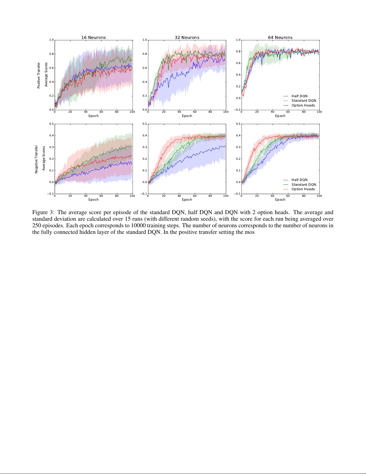
Classifying Options f or Deep Reinf or cement Learning Kai Arulkumaran 1 , Nat Dilokthanakul 2 , Murray Shanahan 2 , and Anil Anthony Bharath 1 1 Department of Bioengineering 2 Department of Computing Imperial College London, London SW7 2BP , UK { kailash.arulkumaran13,n.dilokthanakul14,m.shanahan,a.bharath } @imperial.ac.uk Abstract In this paper we combine one method for hi- erarchical reinforcement learning—the options framew ork—with deep Q-networks (DQNs) through the use of different “option heads” on the policy network, and a supervisory network for choosing between the dif ferent options. W e utilise our setup to inv estigate the ef fects of architectural constraints in subtasks with positiv e and negati v e transfer , across a range of network capacities. W e empirically sho w that our augmented DQN has lower sample complexity when simultaneously learning subtasks with negati ve transfer , without degrading performance when learning subtasks with positiv e transfer . 1 Introduction Recent advances in reinforcement learning have focused on using deep neural networks to represent the state-action v alue function (Q-function) [ Mnih et al. , 2015 ] or a polic y func- tion [ Levine et al. , 2015 ] . The successes of such methods are largely attributed to the representational power of deep networks. It is tempting to create an ultimate end-to-end so- lution to general problems with these kinds of po werful mod- els. Ho we ver , these general methods require large amount of samples in order to learn effecti v e policies. In order to reduce sample complexity , one can use domain knowledge to construct an algorithm that is biased tow ards promising solutions. The deep Q-network (DQN) [ Mnih et al. , 2015 ] is an end-to-end reinforcement learning algorithm that has achieved great success on a variety of video games [ Bellemare et al. , 2013 ] . In this work, we e xplore the possi- bility of imposing some structural priors onto the DQN as a way of adding domain knowledge, whilst trying to limit the reduction in generality of the DQN. In classical reinforcement learning literature, there is a large amount of research focusing on temporal abstraction of problems, which is known under the umbrella of hierar- chical reinforcement learning. The options framew ork [ Sut- ton et al. , 1999 ] augments the set of admissible actions with temporally-extended actions that are called options. In this context, an option is a closed-loop controller that can ex e- cute either primitive actions or other options according to its policy . The ability to use options giv es the agent many ad- vantages, such as temporally-extended exploration, allowing planning across a range of time scales and the ability to trans- fer knowledge to dif ferent tasks. Another approach, MAXQ [ Dietterich, 2000 ] , decomposes a task into a hierarchy of subtasks. This decomposition allo ws MAXQ agents to impro ve performance tow ards achieving the main objecti ve by recursiv ely solving smaller problems first. Both the options and MAXQ frameworks are constructed so that prior domain knowledge can be implemented naturally . Both approaches can be viewed as constructing a main policy from smaller sub-policies with implemented prior kno wledge on either the structural constraints or the behaviour of the sub- policies themselves. W e consider the class of problems where the task can be broken down into re ward-independent subtasks by a human expert. The task decomposition is done such that the sub- tasks share the same state space, but can be explicitly parti- tioned (for different options). If the action space can similarly be partitioned, then this knowledge can also be incorporated to bound the actions av ailable to each option policy . With this domain knowledge we decompose the DQN into a com- position of smaller representations, derived from prior work on hierarchical reinforcement learning. Although there is ev- idence that the DQN can implicitly learn options [ Zahavy et al. , 2016 ] , we in vestigate whether there is an y benefit to con- structing options explicitly . 1.1 Related W ork Our “option heads” are inspired by Osband et al. [ 2016 ] . Their policy network is similar to ours, but without the ad- ditional supervisory network. Their network’ s “bootstrap heads” are used with different motiv ations. They train each of the heads, with dif ferent initialisations, on the same task. This allows the network to represent a distribution over Q- functions. Exploration is done “deeply” by sampling one head and using its policy for the whole episode, while the experiences are shared across the heads. Our motiv ation for using option heads, howe ver , is for allowing the use of tem- porally abstracted actions akin to the options framework, or more concretely , as a way to decompose the policy into a combination of simpler sub-policies. This motiv ates the use of a supervisory network, which is discussed in Subsection 3.2. Although we focus on the options framew ork and the no- tion of subtasks , an alternative view is that of multitask learn- ing. In the context of deep reinforcement learning, recent work has generalised distillation [ Hinton et al. , 2015 ] , ap- plied to classification, in order to train DQNs on sev eral Atari games in parallel [ Rusu et al. , 2015; Parisotto et al. , 2015 ] . Distillation uses trained teacher networks to provide extra training signals for the student network, where origi- nally the technique was used to distill the knowledge from a large teacher netw ork into a smaller student network as a form of model compression. For multitask learning, Parisotto et al. [ 2015 ] were able to keep the student DQN architecture the same as that of the teacher DQNs, whilst Rusu et al. [ 2015 ] created a larger network with an additional fully connected layer . The latter explicitly separated the top of the network into different “controllers” per game, and called the architec- ture a Multi-DQN, and the architecture in combination with their policy distillation algorithm Multi-Dist. Both studies showed that the use of teacher networks could enable learn- ing effecti ve policies on several Atari games in parallel—8 on a standard DQN [ Parisotto et al. , 2015 ] and 10 on a Multi- DQN [ Rusu et al. , 2015 ] . The same architectures were unable to perform well across all games without teacher networks. W e note that the bootstrapped DQN and the multi-DQN hav e similar structures: sev eral “heads” either directly or in- directly abov e shared con volutional layers. One of the base- lines for ev aluating the actor-mimic framew ork [ Parisotto et al. , 2015 ] is the Multitask Conv olutional DQN (MCDQN), which has the same architecture as the bootstrapped DQN. Although working from the same architecture, our goals are different due to incorporating the DQN into the op- tions frame work. The first major dif ference in our work is that we use a supervisory network, which allo ws us to infer which subtask should be attempted at each time step during ev aluation. Con versely , in a multitask setting, dif- ferent tasks are typically clearly separated. Secondly , our method does not rely on teacher networks, instead focus- ing on a DQN whose augmented training signal is based only on the kno wledge of the current subtask. W ith re- spect to the latter point, we focus our analysis on controlling the capacity of the networks, as opposed to scaling param- eters linearly with the number of tasks [ Rusu et al. , 2015; Parisotto et al. , 2015 ] . Another notable success in subtask learning with multi- ple independent sources of reward are univ ersal value func- tion approximators (UVF As) [ Schaul et al. , 2015 ] . UVF As allow the generalisation of value functions across different goals, which helps the agent accomplish tasks that it has nev er seen before. The focus of UVF As is in generalising be- tween similar subtasks by sharing the representation between the dif ferent tasks. This has recently been expanded upon in the hierarchical-DQN [ Kulkarni et al. , 2016 ] ; howe ver , these goal-based approaches have been demonstrated in domains where the dif ferent goals are highly related. From a function approximation perspecti ve, goals should share a lot of struc- ture with the raw states. In contrast, our approach focuses on separating out distinct subtasks, where partial independence between subpolicies can be enforced through structural con- straints. In particular , we expect that separate Q-functions are less prone to negati ve transfer between subtasks. 2 Background Consider a reinforcement learning problem, where we want to find an agent’ s policy π which maximises the expected dis- counted rew ard, E [ R ] = E [ P t γ t r t ] . The discount parame- ter , γ ∈ [0 , 1] , controls the importance of immediate rewards relativ e to more distant rewards in the future. The rew ard r t is a scalar value emitted from a state s t ∈ S . The policy se- lects and performs an action a t ∈ A in response to the state s t , which then transitions to s t +1 . The transition of states is modelled as a Markov decision process (MDP) where each state is a sufficient statistic of the entire history , so that the transition at time t need only depend on s t − 1 and the action a t − 1 . See [ Sutton and Barto, 1998 ] for a full introduction. The Q-learning algorithm [ W atkins, 1989 ] solves the re- inforcement learning problem by approximating the optimal state-action v alue or Q-function, Q ∗ ( s t , a t ) , which is defined as the expected discounted reward starting from state s t and taking initial action a t , and henceforth following the optimal policy π ∗ : Q ∗ ( s t , a t ) = E [ R t | s t , a t , π ∗ ] The Q-function must satisfy the Bellman equation, Q ∗ ( s t , a t ) = E s t +1 [ r t + γ max a t +1 Q ∗ ( s t +1 , a t +1 )] . W e can approximate the Q-function with a function approx- imator Q ( s, a ; θ ) , with parameters θ . Learning is done by adjusting the parameters in such a way to reduce the inconsis- tency between the left and the right hand sides of the Bellman equation. The optimal policy can be deriv ed by simply choos- ing the action that maximises Q ∗ ( s, a ) at each time step. 2.1 Deep Q-networks The DQN [ Mnih et al. , 2015 ] is a con volutional neural net- work that represents the Q-function Q ( s, a ; θ ) with parame- ters θ . The (online) network is trained by minimising a se- quence of loss functions at iteration i : L i ( θ i ) = E s,a,r,s 0 [( y i − Q ( s, a ; θ i )) 2 ] y i = r + γ max a 0 Q ( s 0 , a 0 ; θ − ) (1) The parameters θ − are associated with a separate target network, which is updated with θ i ev ery τ steps. The target network increases the stability of the learning. The param- eters θ i are updated with mini-batch stochastic gradient de- scent following the gradient of the loss function. Another key to the successful training of DQNs is the use of experience replay [ Lin, 1992 ] . Updating the parameters, θ i , with stochastic gradient descent on the squared loss func- tion implies an i.i.d. assumption which is not v alid in an online reinforcement learning problem. Experience replay stores samples of past transitions in a pool. While training, samples are drawn uniformly from this pool. This helps break the temporal correlation between samples and also allows up- dates to reuse samples sev eral times. IJCAI 2016 W orkshop on Deep Reinforcement Learning: Frontiers and Challenges 2.2 Double Deep Q-networks W e follo w the learning algorithm by v an Hasselt et al. [ 2015 ] to lower the overestimation of Q-values in the update rule. This modifies the original target, Equation 1, to the follo wing, y i = r + γ Q ( s 0 , arg max a 0 Q ( s 0 , a 0 ; θ i ); θ − ) . 2.3 The Options Framework The orginal definition of options [ Sutton et al. , 1999 ] consists of three components: a policy , π , a termination condition, β , and an initiation set, I . W e illustrate the role of these compo- nents by following the interpretation by Daniel et al. [ 2012 ] . Consider a stochastic policy , π ( a t | s t ) , or a distribution ov er actions, a t , giv en state, s t , at time step t . W e add an aux- iliary variable, o t ∈ O , such that a t is dependent on o t , and, o t is dependent on s t and o t − 1 . This variable o t controls the selection of action a t through their conditional dependence, π ( a t | s t , o t ) , and can be interpreted as the polic y of a Mark ov option o t . The termination condition, β , can be thought of as a specific constraint of the conditional form, imposed on the transition of the option as follows: π ( o t | o t − 1 , s t ) ∝ β ( s t , o t − 1 ) π ( o t | s t ) + δ o t ,o t − 1 (1 − β ( s t , o t − 1 )) , where δ o t ,o t − 1 is 1 when o t = o t − 1 and 0 otherwise. The initiation set specifies the domain of s t av ailable to π ( o t | s t ) . W e consider a fully observable MDP where s t is assumed to be a sufficient statistic for all the history before t , including o t − 1 . Therefore, we can model o t to be conditionally inde- pedent of o t − 1 giv en s t . W e define our “supervisory policy” as π ( o t | s t ) . Both the termination condition and the initiation set are absorbed into the supervisory policy . The full policy is then decomposed into: π ( a t | s t ) = X o t π ( o t | s t ) π ( a t | o t , s t ) . This form of policy can be seen as a combination of option policies, weighted by the supervisory policy . W e will show in the next section ho w we decompose the DQN into separate option policies, alongside a supervisory policy . 3 Deep Q-networks with Option Heads W e augment the standard DQN with se veral distinct sets of outputs; concretely we use the same architecture as the bootstrapped DQN [ Osband et al. , 2016 ] or the MCDQN [ Parisotto et al. , 2015 ] . As with the MCDQN, we use domain knowledge to choose the number of heads a priori, and use this same knowledge to train each option head separately . A comparison between a standard DQN and a DQN with option heads that we use is pictured in Figure 1. As noted in [ Rusu et al. , 2015 ] , even this augmentation can fail in a multitask setting with different policies interfering at the lower levels of the network, which highlights the need for further study . Along with other work on the DQN, we assume that the con volutional layers learn a general representation of the state space, whilst the fully connected layers at the top of the net- work encode most of the actual policy . In the multitask Atari Figure 1: Comparison of DQN architectures. a) Standard DQN. b) DQN with 2 option heads. setting, the set of games are so different that the states are un- likely to have many features in common [ Rusu et al. , 2015 ] , but we would assume that in a hierarchical reinforcement learning setting with subtasks this problem does not occur . In addition to our augmented policy network , Q o ( s, a ) : O × S × A → R , where o indexes over option heads, we also introduce a supervisory network , O ( s ) : S → O , which learns a mapping from a state to an option; this allows each option head to focus on a subset of the state space. With our networks, our full policy can be written as a deterministic mapping, π ( s ) : S → A , π ( s ) = arg max a Q O ( s ) ( s, a ) 3.1 Option Heads The option heads consist of fully connected layers which branch out from the topmost shared conv olution layer . The final layer of each head outputs the Q-value for each dis- crete action av ailable, and hence can be limited using do- main knowledge of the task at hand and the desired options. While training, an oracle is used to choose which option head should be e valuated at each time step t . The action a t is picked with the  -greedy strategy on the o t head, where  is shared between all heads. The experience samples are tuples of ( s t , a t , s t +1 , r t ) , and are stored in separate experience re- play buf fers for each head. During ev aluation the oracle is replaced with the decisions of the supervisory network. 3.2 Supervisory Network The supervisory network is an arbitrary neural network clas- sifier which represents the supervisory policy . The input layer IJCAI 2016 W orkshop on Deep Reinforcement Learning: Frontiers and Challenges Figure 2: 8 frames of Catch. The first row shows the white ball subtask, and the second ro w sho ws the grey ball subtask. receiv es the entire state. The hidden layers can be constructed using domain knowledge, e.g. con v olutional layers for visual domains. The output layer is a softmax layer which outputs the distribution over options, o t , giv en the state, s t , and can be trained with the standard cross-entropy loss function. During training the targets are gi ven from an oracle. 4 Experiments For our experiments we reimplemented the game of “Catch” [ Mnih et al. , 2014 ] , where the task is to control a paddle at the bottom of the screen to catch falling balls (see Figure 2). The input is a gre yscale 24x24 pixel grid, and the action space consists of 3 discrete actions: move left, mov e right and a no- op. As in [ Mnih et al. , 2015 ] , the DQN recei ves a stack of the current plus previous 3 frames. During each episode a 1 pixel ball f alls randomly from the top of the screen, and the agent’ s 2-pixel-wide paddle must mov e horizontally to catch it. In the original a reward of +1 is giv en for catching a white ball; we add an additional grey ball to introduce subtasks into the en vironment. This simple en vironment allo ws us to meaning- fully ev aluate the effects of the architecture on subtasks with positive and ne gative transfer . F or the positive transfer case the subtasks are the same—catching either ball results in a rew ard of +1. In the negativ e transfer case the grey ball still giv es a reward of +1, but catching the white ball results in a rew ard of -1. In this subtask the optimal agent must learn to catch the grey balls and avoid the perceptually-similar white balls; suboptimal solutions would include avoiding or catch- ing both types of balls. In both setups the type of ball used is switched ev ery episode. Our baseline is the standard DQN. In order to provide a fair comparison, we impose one condition on the architecture of our policy network, and one condition on its training. For the first condition we divide the number of neurons in the hid- den layer of each option head by the number of option heads, thereby keeping the number of parameters the same. For the second condition we alternate heads when performing the Q- learning update, keeping the number of training samples the same. W e also construct a “half DQN”, which contains half the parameters of the standard DQN in the fully connected hidden layer; this uses the standard architecture, not the op- tion heads. This tests whether the sample complexity of our DQN with option heads is either the result of having fewer parameters to tune in each head, or the result of our imposed structural constraint. More details on the model architectures and training hyperparameters are gi ven in the Appendix. As well as in vestigating the effects of different kinds of transfer , we also look into the effects of varying the capac- ity of the network—specifically we run experiments with 16, 32, and 64 neurons in the fully connected hidden layer of the standard DQN. Correspodingly , the half DQN has 8, 16, and 32 neurons, and each of the 2 option heads in our network also has 8, 16, and 32 neurons. As seen in Figure 3, lack of capacity has the most signif- icant effect on performance. As capacity increases, the dif- ferences between the three networks diminishes. Besides ca- pacity , architecture does not appear to have any significant impact on the positiv e transfer subtasks. Howe ver , with neg- ativ e transfer subtasks the DQN with option heads is able to make significantly quicker progress than the standard DQN. When giv en enough capacity , our control for “head capac- ity” in this e xperiment—the half DQN—also con ver ges to the same policy in terms of performance, but with a larger sample complexity . This suggests that incorporating domain knowl- edge in the form of structural constraints can be beneficial, ev en whilst keeping model capacity the same—in particular , the quicker learning suggests that this knowledge can effec- tiv ely be utilised to reduce the number of samples needed in deep reinforcement learning. Qualitativ ely , the conv olutional filters learned by all DQNs are highly similar . This reinforces the intuition that the struc- tural constraint imposed upon the DQN with option heads allows low-le vel feature knowledge about falling balls and moving the paddle to be learned in the shared con volution layers, whilst policies for catching and avoiding balls are rep- resented more explicitly in each head. As the classification task for the supervisory network is simple in this domain, we do not attempt to replace it with an oracle during ev aluation. In practice the network learns to divide the state space rapidly . 5 Discussion W e show that with a simple architectural adjustment, it is pos- sible to successfully impose prior domain knowledge about subtasks into the DQN algorithm. W e demonstrate this idea in a game of catch, where the task of catching or av oiding falling balls depending on their colour can be decomposed intuitiv ely into the subtask of catching gre y balls and another subtask of a voiding white balls—subtasks that incur neg ativ e transfer . W e show that learning the subtasks separately on dif- ferent option heads allows the DQN to learn with lo wer sam- ple complexity . The shared conv olutional layers learn gener- ally useful features, whilst the heads learn to specialise. In comparison, the standard DQN presumably suffers from sub- task interference with only a single Q-function. Additionally , the structural constraint does not hinder performance when learning subtasks with positiv e transfer . Our results are contrary to those reported with the MCDQN trained on eight Atari games simultaneously , which was out- performed by a standard DQN [ Parisotto et al. , 2015 ] . Ac- cording to Parisotto et al. [ 2015 ] , the standard DQN and MCDQN tend to focus on performing well on a subset of games at the expense of the others. W e posit that this “strat- egy” works well for the DQN, whilst the explicitly con- IJCAI 2016 W orkshop on Deep Reinforcement Learning: Frontiers and Challenges 0 20 40 60 80 100 Epoch 0.0 0.2 0.4 0.6 0.8 1.0 Positive Transfer Average Scores 16 Neurons 0 20 40 60 80 100 Epoch 0.0 0.2 0.4 0.6 0.8 1.0 32 Neurons 0 20 40 60 80 100 Epoch 0.2 0.0 0.2 0.4 0.6 0.8 1.0 64 Neurons Half DQN Standard DQN Option Heads 0 20 40 60 80 100 Epoch 0.1 0.0 0.1 0.2 0.3 0.4 0.5 Negative Transfer Average Scores 0 20 40 60 80 100 Epoch 0.1 0.0 0.1 0.2 0.3 0.4 0.5 0 20 40 60 80 100 Epoch 0.1 0.0 0.1 0.2 0.3 0.4 0.5 Half DQN Standard DQN Option Heads Figure 3: The av erage score per episode of the standard DQN, half DQN and DQN with 2 option heads. The av erage and standard deviation are calculated over 15 runs (with different random seeds), with the score for each run being av eraged over 250 episodes. Each epoch corresponds to 10000 training steps. The number of neurons corresponds to the number of neurons in the fully connected hidden layer of the standard DQN. In the positive transfer setting the most important factor is capacity , not the architecture. As capacity increases the dif ference in performance between the networks diminishes. In the negati ve transfer setting the effect of capacity is strong when capacity is very low , but otherwise the DQN with option heads demonstrates a superior sample complexity o ver the baselines. Best viewed in colour . structed controller heads on the MCDQN receive more con- sistent training signals, which may cause parameter gradients that interfere with each other in the shared con v olutional lay- ers [ Caruana, 2012; Rusu et al. , 2015 ] . This is less of a con- cern in the hierarchical reinforcement learning setting as we assume a more coherent state space across all subtasks. In the regime of subtasks rather than multiple tasks, the DQN with option heads is not as generalisable as goal-based approaches [ Schaul et al. , 2015; Kulkarni et al. , 2016 ] . How- ev er , these methods currently require a hand-crafted represen- tation of the goals as input for their networks—a sensible ap- proach only when the goal representation can be reasonably appended to the state space. In contrast, our oracle mapping from states to options can be used when constructing rep- resentations of goals as inputs is not a straightforward task. This suggests future work in removing the oracle by focus- ing on option discovery , where the agent must learn options without the use of a supervisory signal. Acknowledgements The authors gratefully ackno wledge a gift of equipment from NVIDIA Corporation and the support of the EPSRC CDT in Neurotechnology . References [ Bellemare et al. , 2013 ] Marc G Bellemare, Y a var Naddaf, Joel V eness, and Michael Bowling. The Arcade Learning En vironment: An Ev aluation Platform for General Agents. Journal of Artificial Intelligence Resear ch , 47:253–279, 2013. [ Caruana, 2012 ] Rich Caruana. A dozen tricks with multi- task learning. In Neural Networks: T ric ks of the T rade , pages 163–189. Springer , 2012. [ Daniel et al. , 2012 ] Christian Daniel, Gerhard Neumann, and Jan R Peters. Hierarchical relativ e entropy policy search. In International Confer ence on Artificial Intelli- gence and Statistics , pages 273–281, 2012. [ Dietterich, 2000 ] Thomas G Dietterich. Hierarchical rein- forcement learning with the MAXQ value function de- composition. Journal of Artificial Intelligence Resear ch , 13:227–303, 2000. [ Hinton et al. , 2015 ] Geoffre y Hinton, Oriol V inyals, and Jeff Dean. Distilling the knowledge in a neural network. arXiv pr eprint arXiv:1503.02531 , 2015. IJCAI 2016 W orkshop on Deep Reinforcement Learning: Frontiers and Challenges [ Kulkarni et al. , 2016 ] T ejas D Kulkarni, Karthik R Narasimhan, Ardavan Saeedi, and Joshua B T enenbaum. Hierarchical Deep Reinforcement Learning: Integrating T emporal Abstraction and Intrinsic Motiv ation. arXiv pr eprint arXiv:1604.06057 , 2016. [ Levine et al. , 2015 ] Serge y Le vine, Chelsea Finn, T rev or Darrell, and Pieter Abbeel. End-to-end training of deep visuomotor policies. arXiv pr eprint arXiv:1504.00702 , 2015. [ Lin, 1992 ] Long-Ji Lin. Self-improving reactiv e agents based on reinforcement learning, planning and teaching. Machine learning , 8(3-4):293–321, 1992. [ Mnih et al. , 2014 ] V olodymyr Mnih, Nicolas Heess, Alex Grav es, et al. Recurrent models of visual attention. In Ad- vances in Neural Information Processing Systems , pages 2204–2212, 2014. [ Mnih et al. , 2015 ] V olodymyr Mnih, Koray Kavukcuoglu, David Silver , Andrei A Rusu, Joel V eness, Marc G Belle- mare, Alex Grav es, Martin Riedmiller, Andreas K Fidje- land, Georg Ostro vski, et al. Human-level control through deep reinforcement learning. Nature , 518(7540):529–533, 2015. [ Osband et al. , 2016 ] Ian Osband, Charles Blundell, Alexan- der Pritzel, and Benjamin V an Roy . Deep Exploration via Bootstrapped DQN. arXiv pr eprint arXiv:1602.04621 , 2016. [ Parisotto et al. , 2015 ] Emilio Parisotto, Jimmy Lei Ba, and Ruslan Salakhutdinov . Actor -Mimic: Deep Multitask and T ransfer Reinforcement Learning. arXiv pr eprint arXiv:1511.06342 , 2015. [ Rusu et al. , 2015 ] Andrei A Rusu, Sergio Gomez Col- menarejo, Caglar Gulcehre, Guillaume Desjardins, James Kirkpatrick, Razvan Pascanu, V olodymyr Mnih, K oray Kavukcuoglu, and Raia Hadsell. Policy Distillation. arXiv pr eprint arXiv:1511.06295 , 2015. [ Schaul et al. , 2015 ] T om Schaul, Daniel Horgan, Karol Gregor , and David Silver . Univ ersal V alue Function Approximators. In Pr oceedings of the 32nd Interna- tional Conference on Machine Learning (ICML-15) , pages 1312–1320, 2015. [ Sutton and Barto, 1998 ] Richard S Sutton and Andrew G Barto. Reinfor cement learning: An intr oduction . MIT press, 1998. [ Sutton et al. , 1999 ] Richard S Sutton, Doina Precup, and Satinder Singh. Between MDPs and semi-MDPs: A framew ork for temporal abstraction in reinforcement learning. Artificial intelligence , 112(1):181–211, 1999. [ V an Hasselt et al. , 2015 ] Hado V an Hasselt, Arthur Guez, and David Silver . Deep reinforcement learning with dou- ble Q-learning. arXiv preprint , 2015. [ W atkins, 1989 ] Christopher John Cornish Hellaby W atkins. Learning fr om delayed r e war ds . PhD thesis, Univ ersity of Cambridge England, 1989. [ Zahavy et al. , 2016 ] T om Zahavy , Nir Ben Zrihem, and Shie Mannor . Graying the black box: Understanding DQNs. arXiv preprint , 2016. A ppendix A Model W e use a smaller DQN than the one specified in [ Mnih et al. , 2015 ] . The baseline (standard) DQN architecture that we used in our experiments, with a capacity of “32 neurons”, is as follows: Layer Specification 1 32 5x5 spatial con volution, 2x2 stride, 1x1 zero-padding, ReLU 2 32 5x5 spatial con volution, 2x2 stride, ReLU 3 32 fully connected, ReLU 4 3 fully connected As our version of Catch can be divided into 2 distinct sub- tasks, our policy network therefore has 2 option heads. Each option head has 16 neurons each in the penultimate fully con- nected layers—half that of the baseline DQN. The half DQN therefore also has 16 neurons in the penultimate fully con- nected layer . The same formula is employed when testing with a capacity of 16 and 64 neurons. Unlike [ Osband et al. , 2016 ] , we do not normalise the gra- dients coming through each option head, as the errors are only backpropagated through one head at a time. B Hyperparameters Hyperparameters were originally manually tuned for the model with the original version of Catch [ Mnih et al. , 2014 ] (only white balls giving a reward of +1). W e then performed a hyperparameter search ov er learning rates ∈ { 0.000125, 0.00025, 0.0005 } , target network update frequencies ∈ { 4, 32, 128 } , and final values of  ∈ { 0.01, 0.05 } . The learning rate with the best performance for all models was 0.00025, except for the standard DQN and half DQN in the negativ e transfer setting, where 0.000125 was better . This is an inter- esting finding—with negati ve transfer the standard architec- ture requires a lower learning rate, whilst with option heads a higher learning rate can still be used. The follo wing hyperpa- rameters were used for all models, where only hyperparame- ters that differ from those used in [ V an Hasselt et al. , 2015 ] for the tuned double DQN are giv en: Hyperparameters V alue Description Replay memory size 10000 Size of each experience replay memory buf fer . T arget network update frequency 4 Frequency (in number of steps) with which the target network parameters are updated with the policy network parameters. Optimiser Adam Stochastic gradient descent optimiser . Final exploration frame 10000 Number of steps over which  is linearly an- nealed. Replay start size 10000 Number of steps of random e xploration before  is annealed. Gradient clipping 10 Max absolute value of the L2 norm of the gra- dients. V alidation frequency 10000 Number of steps after which evaluation is run. V alidation steps 6000 Number of steps to use during ev aluation. Corresponds to 250 episodes of Catch. IJCAI 2016 W orkshop on Deep Reinforcement Learning: Frontiers and Challenges