Synthesizing Dynamic Patterns by Spatial-Temporal Generative ConvNet

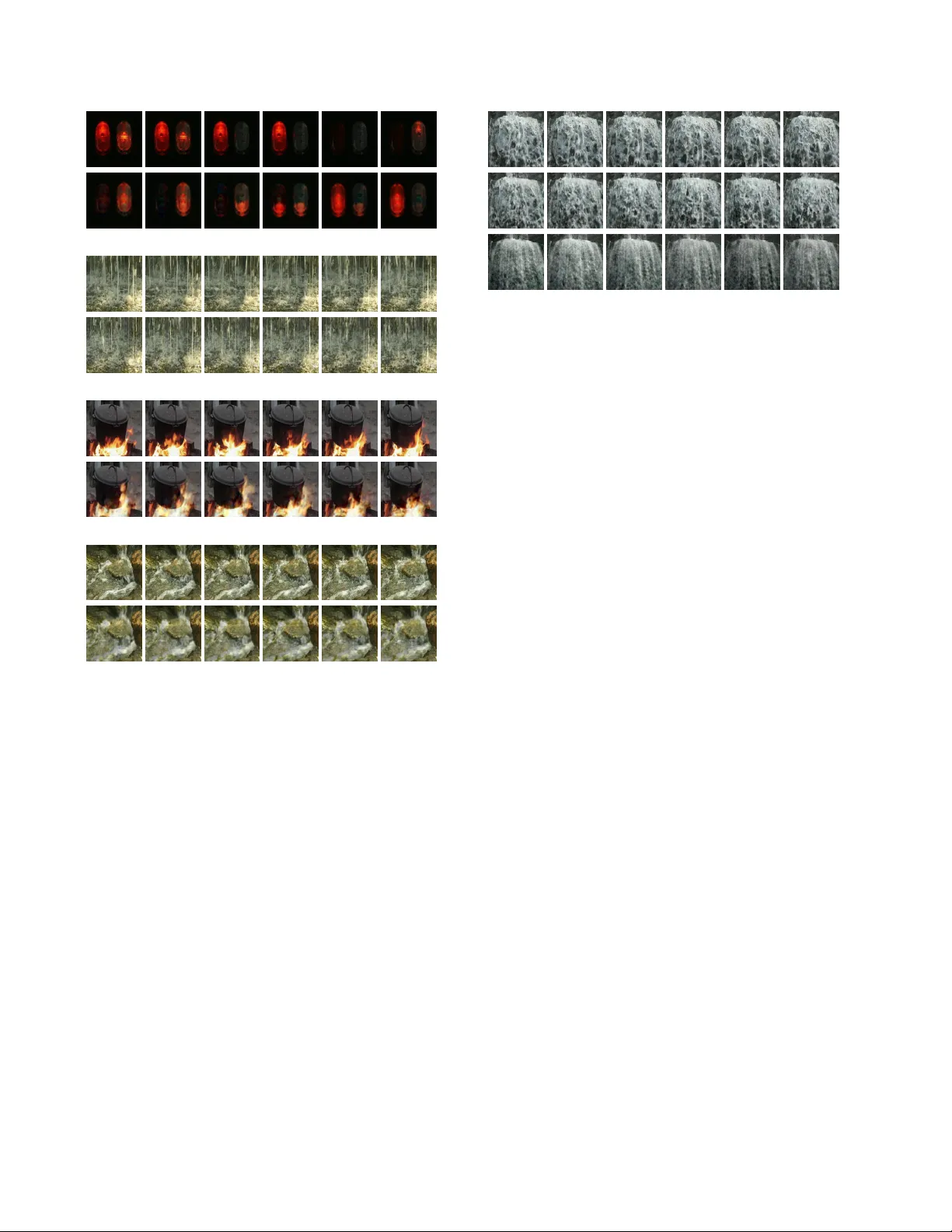
Synthesizing Dynamic Patter ns by Spatial-T emporal Generativ e Con vNet Jianwen Xie, Song-Chun Zhu, and Y ing Nian W u Uni versity of California, Los Angeles (UCLA), USA jianwen@ucla.edu, sczhu@stat.ucla.edu, ywu@stat.ucla.edu Abstract V ideo sequences contain ric h dynamic patterns, such as dynamic textur e patterns that exhibit stationarity in the tem- poral domain, and action patterns that ar e non-stationary in either spatial or tempor al domain. W e show that a spatial- temporal gener ative Con vNet can be used to model and syn- thesize dynamic patterns. The model defines a probability distribution on the video sequence, and the log pr obability is defined by a spatial-temporal Con vNet that consists of multiple layers of spatial-temporal filter s to captur e spatial- temporal patterns of diff er ent scales. The model can be learned fr om the training video sequences by an “analysis by synthesis” learning algorithm that iterates the follow- ing two steps. Step 1 synthesizes video sequences fr om the curr ently learned model. Step 2 then updates the model pa- rameters based on the differ ence between the synthesized video sequences and the observed training sequences. W e show that the learning algorithm can synthesize r ealistic dynamic patterns. 1. Introduction There are a wide v ariety of dynamic patterns in video sequences, including dynamic textures [ 2 ] or textured mo- tions [ 24 ] that exhibit statistical stationarity or stochastic repetiti veness in the temporal dimension, and action patterns that are non-stationary in either spatial or temporal domain. Synthesizing and analyzing such dynamic patterns has been an interesting problem. In this paper , we focus on the task of synthesizing dynamic patterns using a generative v ersion of the con volutional neural netw ork (Con vNet or CNN). The ConvNet [ 14 , 12 ] has prov en to be an immensely successful discriminati ve learning machine. The con volution operation in the Con vNet is particularly suited for signals such as images, videos and sounds that e xhibit translation in- variance either in the spatial domain or the temporal domain or both. Recently , researchers hav e become increasingly interested in the generati ve aspects of Con vNet, for the pur- pose of visualizing the kno wledge learned by the Con vNet, or synthesizing realistic signals, or developing generativ e models that can be used for unsupervised learning. In terms of synthesis, various approaches based on the Con vNet have been proposed to synthesize realistic static images [ 3 , 7 , 1 , 13 , 16 ]. Howe ver , there has not been much work in the literature on synthesizing dynamic patterns based on the Con vNet, and this is the focus of the present paper . Specifically , we propose to synthesize dynamic patterns by generalizing the generativ e Con vNet model recently pro- posed by [ 29 ]. The generativ e Con vNet can be derived from the discriminativ e Con vNet. It is a random field model or an energy-based model [ 15 , 20 ] that is in the form of e xponen- tial tilting of a reference distribution such as the Gaussian white noise distrib ution or the uniform distribution. The exponential tilting is parametrized by a Con vNet that in- volv es multiple layers of linear filters and rectified linear units (ReLU) [ 12 ], which seek to capture features or patterns at different scales. The generativ e Con vNet can be sampled by the Langevin dynamics. The model can be learned by the stochastic gradi- ent algorithm [ 31 ]. It is an “analysis by synthesis” scheme that seeks to match the synthesized signals generated by the Langevin dynamics to the observed training signals. Specifi- cally , the learning algorithm iterates the following two steps after initializing the parameters and the synthesized signals. Step 1 updates the synthesized signals by the Langevin dy- namics that samples from the currently learned model. Step 2 then updates the parameters based on the difference be- tween the synthesized data and the observed data in order to shift the density of the model from the synthesized data tow ards the observed data. It is shown by [ 29 ] that the learn- ing algorithm can synthesize realistic spatial image patterns such as textures and objects. In this article, we generalize the spatial generati ve Con- vNet by adding the temporal dimension, so that the resulting Con vNet consists of multiple layers of spatial-temporal fil- ters that seek to capture spatial-temporal patterns at various scales. W e show that the learning algorithm for training the spatial-temporal generativ e Con vNet can synthesize realistic dynamic patterns. W e also show that it is possible to learn the model from incomplete video sequences with either oc- cluded pixels or missing frames, so that model learning and 1 pattern completion can be accomplished simultaneously . 2. Related work Our work is a generalization of the generati ve Con vNet model of [ 29 ] by adding the temporal dimension. [ 29 ] did not w ork on dynamic patterns such as those in the video sequences. The spatial-temporal discriminativ e Con vNet was used by [ 11 ] for analyzing video data. The connection between discriminati ve ConvNet and generativ e Con vNet was studied by [ 29 ]. Dynamic te xtures or textured motions have been stud- ied by [ 2 , 24 , 25 , 9 ]. For instance, [ 2 ] proposed a vector auto-regressi ve model coupled with frame-wise dimension reduction by single v alue decomposition. It is a linear model with Gaussian innov ations. [ 24 ] proposed a dynamic model based on sparse linear representation of frames. See [ 30 ] for a recent revie w of dynamic textures. The spatial-temporal generati ve Con vNet is a non-linear and non-Gaussian model and is e xpected to be more flexible in capturing complex spatial-temporal patterns in dynamic textures with multiple layers of non-linear spatial-temporal filters. Recently [ 23 ] generalized the generati ve adv ersarial net- works [ 6 ] to model dynamic patterns. Our model is an energy-based model and it also has an adversarial interpreta- tion. See section 3.4 for details. For temporal data, a popular model is the recurrent neural network [ 27 , 10 ]. It is a causal model and it requires a start- ing frame. In contrast, our model is non-causal, and does not require a starting frame. Compared to the recurrent net- work, our model is more con venient and direct in capturing temporal patterns at multiple time scales. 3. Spatial-temporal generative Con vNet 3.1. Spatial-temporal filters T o fix notation, let I ( x, t ) be an image sequence of a video defined on the square (or rectangular) image domain D and the time domain T , where x = ( x 1 , x 2 ) ∈ D index es the coordinates of pixels, and t ∈ T index es the frames in the video sequence. W e can treat I ( x, t ) as a three dimensional function defined on D × T . For a spatial-temporal filter F , we let F ∗ I denote the filtered image sequence or feature map, and let [ F ∗ I ]( x, t ) denote the filter response or feature at pixel x and time t . The spatial-temporal ConvNet is a composition of mul- tiple layers of linear filtering and ReLU non-linearity , as expressed by the follo wing recursi ve formula: [ F ( l ) k ∗ I ]( x, t ) = h N l − 1 X i =1 X ( y ,s ) ∈S l w ( l,k ) i,y ,s × [ F ( l − 1) i ∗ I ]( x + y , t + s ) + b l,k ! , (1) where l ∈ { 1 , 2 , ..., L } index es the layers. { F ( l ) k , k = 1 , ..., N l } are the filters at layer l , and { F ( l − 1) i , i = 1 , ..., N l − 1 } are the filters at layer l − 1 . k and i are used to index filters at layers l and l − 1 respectiv ely , and N l and N l − 1 are the numbers of filters at layers l and l − 1 respectiv ely . The filters are locally supported, so the range of ( y , s ) is within a local support S l (such as a 7 × 7 × 3 box of image sequence). The weight parameters ( w ( l,k ) i,y ,s , ( y , s ) ∈ S l , i = 1 , ..., N l − 1 ) define a linear filter that operates on ( F ( l − 1) i ∗ I , i = 1 , ..., N l − 1 ) . The linear fil- tering operation is follo wed by ReLU h ( r ) = max(0 , r ) . At the bottom layer , [ F (0) k ∗ I ]( x, t ) = I k ( x, t ) , where k ∈ { R , G , B } index es the three color channels. Sub- sampling may be implemented so that in [ F ( l ) k ∗ I ]( x, t ) , x ∈ D l ⊂ D , and t ∈ T l ⊂ T . The spatial-temporal filters at multiple layers are expected to capture the spatial-temporal patterns at multiple scales. It is possible that the top-layer filters are fully connected in the spatial domain as well as the temporal domain (e.g., the feature maps are 1 × 1 in the spatial domain) if the dynamic pattern does not exhibit spatial or temporal stationarity . 3.2. Spatial-temporal generative Con vNet The spatial-temporal generativ e Con vNet is an energy- based model or a random field model defined on the image sequence I = ( I ( x, t ) , x ∈ D , t ∈ T ) . It is in the form of exponential tilting of a reference distrib ution q ( I ) : p ( I ; w ) = 1 Z ( w ) exp [ f ( I ; w )] q ( I ) , (2) where the scoring function f ( I ; w ) is f ( I ; w ) = K X k =1 X x ∈D L X t ∈T L [ F ( L ) k ∗ I ]( x, t ) , (3) where w consists of all the weight and bias terms that define the filters ( F ( L ) k , k = 1 , ..., K = N L ) at layer L , and q is the Gaussian white noise model, i.e., q ( I ) = 1 (2 π σ 2 ) |D×T | / 2 exp  − 1 2 σ 2 || I || 2  , (4) where |D × T | counts the number of pixels in the domain D × T . W ithout loss of generality , we shall assume σ 2 = 1 . The scoring function f ( I ; w ) in ( 3 ) tilts the Gaussian reference distribution into a non-Gaussian model. In fact, the purpose of f ( I ; w ) is to identify the non-Gaussian spatial- temporal features or patterns. In the definition of f ( I ; w ) in ( 3 ), we sum over the filter responses at the top layer L ov er all the filters, positions and times. The spatial and temporal pooling reflects the fact that we assume the model is stationary in spatial and temporal domains. If the dynamic texture is non-stationary in the spatial or temporal domain, then the top layer filters F ( L ) k are fully connected in the spatial or temporal domain, e.g., D L is 1 × 1 . A simple but consequential property of the ReLU non- linearity is that h ( r ) = max(0 , r ) = 1( r > 0) r , where 1() is the indicator function, so that 1( r > 0) = 1 if r > 0 and 0 otherwise. As a result, the scoring func- tion f ( I ; w ) is piecewise linear [ 17 ], and each linear piece is defined by the multiple layers of binary activ ation vari- ables δ ( l ) k,x,t ( I ; w ) = 1  [ F ( l ) k ∗ I ]( x, t ) > 0  , which tells us whether a local spatial-temporal pattern represented by the k -th filter at layer l , F ( l ) k , is detected at position x and time t . Let δ ( I ; w ) =  δ ( l ) k,x,t ( I ; w ) , ∀ l, k , x, t  be the activ ation pattern of I . Then δ ( I ; w ) divides the image space into a large number of pieces according to the v alue of δ ( I ; w ) . On each piece of image space with fixed δ ( I ; w ) , the scoring function f ( I ; w ) is linear , i.e., f ( I ; w ) = a w,δ ( I ; w ) + h I , B w,δ ( I ; w ) i , (5) where both a and B are defined by δ ( I ; w ) and w . In fact, B = ∂ f ( I ; w ) /∂ I , and can be computed by back- propagation, with h 0 ( r ) = 1( r > 0) . The back-propagation process defines a top-down deconv olution process [ 32 ], where the filters at multiple layers become the basis functions at those layers, and the acti vation variables at dif ferent layers in δ ( I ; w ) become the coef ficients of the basis functions in the top-down decon volution. p ( I ; w ) in ( 2 ) is an ener gy-based model [ 15 , 20 ], whose energy function is a combination of the ` 2 norm k I k 2 that comes from the reference distrib ution q ( I ) and the piecewise linear scoring function f ( I ; w ) , i.e., E ( I ; w ) = − f ( I ; w ) + 1 2 k I k 2 = 1 2 k I k 2 −  a w,δ ( I ; w ) + h I , B w,δ ( I ; w ) i  = 1 2 k I − B w,δ ( I ; w ) k 2 + const , (6) where const = − a w,δ ( I ; w ) − k B w,δ ( I ; w ) k 2 / 2 , which is con- stant on the piece of image space with fixed δ ( I ; w ) . Since E ( I ; w ) is a piecewise quadratic function, p ( I ; w ) is piecewise Gaussian. On the piece of image space { I : δ ( I ; w ) = δ } , where δ is a fixed v alue of δ ( I ; w ) , p ( I ; w ) is N( B w,δ , 1 ) truncated to { I : δ ( I ; w ) = δ } , where we use 1 to denote the identity matrix. If the mean of this Gaussian piece, B w,δ , is within { I : δ ( I ; w ) = δ } , then B w,δ is also a local mode, and this local mode I satisfies a hierarchical auto- encoder , with a bottom-up encoding process δ = δ ( I ; w ) , and a top-down decoding process I = B w,δ . In general, for an image sequence I , B w,δ ( I ; w ) can be considered a reconstruction of I , and this reconstruction is e xact if I is a local mode of E ( I ; w ) . 3.3. Sampling and learning algorithm One can sample from p ( I ; w ) of model ( 2 ) by the Langevin dynamics: I τ +1 = I τ −  2 2  I τ − B w,δ ( I τ ; w )  + Z τ , (7) where τ index es the time steps,  is the step size, and Z τ ∼ N(0 , 1 ) . The dynamics is dri ven by the reconstruction error I − B w,δ ( I ; w ) . The finiteness of the step size  can be corrected by a Metropolis-Hastings acceptance-rejection step. The Langevin dynamics can be extended to Hamilto- nian Monte Carlo [ 18 ] or more sophisticated versions [ 5 ]. The learning of w from training image sequences { I m , m = 1 , ..., M } can be accomplished by the maximum likelihood. Let L ( w ) = P M m =1 log p ( I ; w ) / M , with p ( I ; w ) defined in ( 2 ), ∂ L ( w ) ∂ w = 1 M M X m =1 ∂ ∂ w f ( I m ; w ) − E w  ∂ ∂ w f ( I ; w )  . (8) The expectation can be approximated by the Monte Carlo samples [ 31 ] produced by the Lange vin dynamics. See Al- gorithm 1 for a description of the learning and sampling al- gorithm. The algorithm keeps synthesizing image sequences from the current model, and updating the model parameters in order to match the synthesized image sequences to the observed image sequences. The learning algorithm keeps shifting the probability density or low ener gy regions of the model from the synthesized data tow ards the observed data. In the learning algorithm, the Langevin sampling step in volv es the computation of ∂ f ( I ; w ) /∂ I , and the parame- ter updating step in volv es the computation of ∂ f ( I ; w ) /∂ w . Because of the ConvNet structure of f ( I ; w ) , both gradi- ents can be computed ef ficiently by back-propagation, and the two gradients share most of their chain rule computa- tions in back-propagation. In term of MCMC sampling, the Lange vin dynamics samples from an e volving distribu- tion because w ( t ) keeps changing. Thus the learning and sampling algorithm runs non-stationary chains. 3.4. Adversarial interpr etation Our model is an energy-based model p ( I ; w ) = 1 Z ( w ) exp[ −E ( I ; w )] . (9) The update of w is based on L 0 ( w ) which can be approxi- mated by 1 ˜ M ˜ M X m =1 ∂ ∂ w E ( ˜ I m ; w ) − 1 M M X m =1 ∂ ∂ w E ( I m ; w ) , (10) where { ˜ I m , m = 1 , ..., ˜ M } are the synthesized image se- quences that are generated by the Langevin dynamics. At Algorithm 1 Learning and sampling algorithm Input: (1) training image sequences { I m , m = 1 , ..., M } (2) number of synthesized image sequences ˜ M (3) number of Langevin steps l (4) number of learning iterations T Output: (1) estimated parameters w (2) synthesized image sequences { ˜ I m , m = 1 , ..., ˜ M } 1: Let t ← 0 , initialize w (0) . 2: Initialize ˜ I m , for m = 1 , ..., ˜ M . 3: repeat 4: For each m , run l steps of Langevin dynamics to update ˜ I m , i.e., starting from the current ˜ I m , each step follows equation ( 7 ). 5: Calculate H obs = P M m =1 ∂ ∂ w f ( I m ; w ( t ) ) / M , and H syn = P ˜ M m =1 ∂ ∂ w f ( ˜ I m ; w ( t ) ) / ˜ M . 6: Update w ( t +1) ← w ( t ) + η t ( H obs − H syn ) , with step size η t . 7: Let t ← t + 1 8: until t = T the zero temperature limit, the Langevin dynamics becomes gradient descent: ˜ I τ +1 = ˜ I τ −  2 2 ∂ ∂ ˜ I E ( ˜ I τ ; w ) . (11) Consider the value function V ( ˜ I m , m = 1 , ..., ˜ M ; w ) : 1 ˜ M ˜ M X m =1 E ( ˜ I m ; w ) − 1 M M X m =1 E ( I m ; w ) . (12) The updating of w is to increase V by shifting the lo w energy regions from the synthesized image sequences { ˜ I m } to the observed image sequences { I m } , whereas the updating of { ˜ I m , m = 1 , ..., ˜ M } is to decrease V by moving the syn- thesized image sequences tow ards the low energy regions. This is an adversarial interpretation of the learning and sam- pling algorithm. It can also be considered a generalization of the herding method [ 26 ] from exponential family models to general energy-based models. In our work, we let −E ( I ; w ) = f ( I ; w ) − k I k 2 / 2 σ 2 . W e can also let −E ( I ; w ) = f ( I ; w ) by assuming a uni- form reference distribution q ( I ) . Our experiments show that the model with the uniform q can also synthesize realistic dynamic patterns. The generative adversarial learning [ 6 , 23 ] has a generator network. Unlike our model which is based on a bottom-up Con vNet f ( I ; w ) , the generator network generates I by a top-down Con vNet I = g ( X ; ˜ w ) where X is a latent vec- tor that follows a known prior distribution, and ˜ w collects (a) riv er (b) ocean Figure 1. Synthesizing dynamic te xtures with both spatial and temporal stationarity . For each category , the first row displays the frames of the observed sequence, and the second and third rows display the corresponding frames of two synthesized sequences generated by the learning algorithm. (a) riv er . (b) ocean. the parameters of the top-down Con vNet. Recently [ 8 ] de- veloped an alternating back-propagation algorithm to train the generator network, without in volving an extra netw ork. More recently , [ 28 ] de veloped a cooperati ve training method that recruits a generator network g ( X ; ˜ w ) to reconstruct and regenerate the synthesized image sequences { ˜ I m } to speed up MCMC sampling. 4. Experiments W e learn the spatial-temporal generati ve Con vNet from video clips collected from DynT ex++ dataset of [ 4 ] and the Internet. The code in the experiments is based on the MatCon vNet of [ 22 ] and MexCon v3D of [ 21 ]. W e show the synthesis results by displaying the frames in the video sequences. W e have posted the synthesis results on the project page http://www.stat.ucla.edu/ ~jxie/STGConvNet/STGConvNet.html , so that the reader can watch the videos. 4.1. Experiment 1: Generating dynamic textures with both spatial and temporal stationarity W e first learn the model from dynamic textures that are stationary in both spatial and temporal domains. W e use spatial-temporal filters that are con volutional in both spatial and temporal domains. The first layer has 120 15 × 15 × 15 filters with sub-sampling size of 7 pixels and frames. The (a) flashing lights (b) fountain (c) burning fire heating a pot (d) spring water Figure 2. Synthesizing dynamic textures with only temporal sta- tionarity . For each category , the first row displays the frames of the observed sequence, and the second ro w displays the corresponding frames of a synthesized sequence generated by the learning algo- rithm. (a) flashing lights. (b) fountain. (c) burning fire heating a pot. (d) spring water . second layer has 40 7 × 7 × 7 filters with sub-sampling size of 3. The third layer has 20 3 × 3 × 2 filters with sub-sampling size of 2 × 2 × 1 . Figure 1 displays 2 results. For each category , the first row displays 7 frames of the observed sequence, while the second and third rows sho w the corre- sponding frames of two synthesized sequences generated by the learning algorithm. W e use the layer-by-layer learning scheme. Starting from the first layer , we sequentially add the layers one by one. Each time we learn the model and generate the synthesized image sequence using Algorithm 1 . While learning the new layer of filters, we refine the lower layers of filters with back-propagation. W e learn a spatial-temporal generativ e Con vNet for each Figure 3. Comparison on synthesizing dynamic texture of w aterfall. From top to bottom: segments of the observed sequence, synthe- sized sequence by our method, and synthesized sequence by the method of [ 2 ]. category from one observed video that is prepared to be of the size 224 × 224 × 50 or 70. The range of intensi- ties is [0, 255]. Mean subtraction is used as pre-processing. W e use ˜ M = 3 chain for Langevin sampling. The num- ber of Langevin iterations between ev ery two consecutiv e updates of parameters, l = 20 . The number of learning iterations T = 1200 , where we add one more layer every 400 iterations. W e use layer-specific learning rates, where the learning rate at the higher layer is less than that at the lower layer , in order to obtain stable con ver gence. 4.2. Experiment 2: Generating dynamic textures with only temporal stationarity Many dynamic te xtures hav e structured background and objects that are not stationary in the spatial domain. In this case, the network used in Experiment 1 may fail. Howe ver , we can modify the network in Experiment 1 by using filters that are fully connected in the spatial domain at the second layer . Specifically , the first layer has 120 7 × 7 × 7 filters with sub-sampling size of 3 pixels and frames. The second layer is a spatially fully connected layer, which contains 30 filters that are fully connected in the spatial domain b ut con volutional in the temporal domain. The temporal size of the filters is 4 frames with sub-sampling size of 2 frames in the temporal dimension. Due to the spatial full connectivity at the second layer , the spatial domain of the feature maps at the third layer is reduced to 1 × 1 . The third layer has 5 1 × 1 × 2 filters with sub-sampling size of 1 in the temporal dimension. W e use end-to-end learning scheme to learn the above 3-layer spatial-temporal generati ve Con vNet for dynamic textures. At each iteration, the 3 layers of filters are updated with 3 different layer-specific learning rates. The learning rate at the higher layer is much less than that at the lo wer layer to av oid the issue of large gradients. W e learn a spatial-temporal generativ e Con vNet for each category from one training video. W e synthesize ˜ M = 3 (a) 21 -st frame of 30 observed sequences (b) 21 -st frame of 30 synthesized sequences (c) 2 examples of synthesized sequences Figure 4. Learning from 30 observed fire videos with mini-batch implementation. videos using the Lange vin dynamics. Figure 2 displays the results. For each category , the first ro w sho ws 6 frames of the observed sequence (224 × 224 × 70), and the second row shows the corresponding frames of a synthesized sequence generated by the learning algorithm. W e use the same set of parameters for all the categories without tuning. Figure 3 compares our method to that of [ 2 ], which is a linear dynamic system model. The image sequence generated by this model appears more blurred than the sequence generated by our method. The learning of our model can be scaled up. W e learn the fire pattern from 30 training videos, with mini-batch implementation. The size of each mini-batch is 10 videos. Each video contains 30 frames ( 100 × 100 pixels). For each mini-batch, ˜ M = 13 parallel chains for Lange vin sampling is used. For this experiment, we slightly modify the network by using 120 11 × 11 × 9 filters with sub-sampling size of 5 pixels and 4 frames at the first layer, and 30 spatially fully connected filters with temporal size of 5 frames and sub-sampling size of 2 at the second layer, while keeping the setting of the third layer unchanged. The number of learning iterations T = 1300 . Figure 4 sho ws one frame for each of 30 observed sequences and the corresponding frame of the synthesized sequences. T wo examples of synthesized sequences are also displayed. 4.3. Experiment 3: Generating action patterns without spatial or temporal stationarity Experiments 1 and 2 show that the generativ e spatial- temporal Con vNet can learn from sequences without align- observed sequences synthesized sequences (a) running cows observed sequences synthesized sequences (b) running tigers Figure 5. Synthesizing action patterns. For each action video se- quence, 6 continuous frames are shown. (a) running cows. Frames of 2 of 5 training sequences are displayed. The corresponding frames of 2 of 8 synthesized sequences generated by the learning algorithm are displayed. (b) running tigers. Frames of 2 observed training sequences are displayed. The corresponding frames of 2 of 4 synthesized sequences are displayed. ment. W e can also specialize it to learning roughly aligned video sequences of action patterns, which are non-stationary in either spatial or temporal domain, by using a single top- layer filter that cov ers the whole video sequence. W e learn a 2-layer spatial-temporal generativ e ConvNet from video sequences of aligned actions. The first layer has 200 7 × 7 × 7 filters with sub-sampling size of 3 pixels and frames. The second layer is a fully connected layer with a single filter that covers the whole sequence. The observed sequences are of the size 100 × 200 × 70 . Figure 5 displays two results of modeling and synthesiz- ing actions from roughly aligned video sequences. W e learn a model for each category , where the number of training sequences is 5 for the running cow example, and 2 for the running tiger example. The videos are collected from the Internet and each has 70 frames. For each example, Figure 5 displays segments of 2 observ ed sequences, and segments of 2 synthesized action sequences generated by the learning al- gorithm. W e run ˜ M = 8 paralleled chains for the experiment of running co ws, and 4 paralleled chains for the experiment of running tigers. The experiments sho w that our model can capture non-stationary action patterns. One limitation of our model is that it does not in volve explicit tracking of the objects and their parts. 4.4. Experiment 4: Learning fr om incomplete data Our model can learn from video sequences with occluded pixels. The task is inspired by the fact that most of the videos contain occluded objects. Our learning method can be adapted to this task with minimal modification. The modification in volves, for each iteration, running k steps of Langevin dynamics to recover the occluded regions of the observed sequences. At each iteration, we use the completed observed sequences and the synthesized sequences to com- pute the gradient of the log-likelihood and update the model parameters. Our method simultaneously accomplishes the following tasks: (1) recover the occluded pix els of the train- ing video sequences, (2) synthesize ne w video sequences from the learned model, (3) learn the model by updating the model parameters using the recov ered sequences and the synthesized sequences. See Algorithm 2 for the description of the learning, sampling, and recov ery algorithm. T able 1. Recov ery errors in occlusion experiments (a) salt and pepper masks ours MRF- ` 1 MRF- ` 2 flag 3.7923 6.6211 10.9216 fountain 5.5403 8.1904 11.3850 ocean 3.3739 7.2983 9.6020 playing 5.9035 14.3665 15.7735 sea world 5.3720 10.6127 11.7803 traffic 7.2029 14.7512 17.6790 windmill 5.9484 8.9095 12.6487 A vg. 5.3048 10.1071 12.8272 (b) single region masks ours MRF- ` 1 MRF- ` 2 flag 8.1636 10.6586 12.5300 fountain 6.0323 11.8299 12.1696 ocean 3.4842 8.7498 9.8078 playing 6.1575 15.6296 15.7085 sea world 5.8850 12.0297 12.2868 traffic 6.8306 15.3660 16.5787 windmill 7.8858 11.7355 13.2036 A vg. 6.3484 12.2856 13.1836 (c) 50 % missing frames ours MRF- ` 1 MRF- ` 2 flag 5.5992 10.7171 12.6317 fountain 8.0531 19.4331 13.2251 ocean 4.0428 9.0838 9.8913 playing 7.6103 22.2827 17.5692 sea world 5.4348 13.5101 12.9305 traffic 8.8245 16.6965 17.1830 windmill 7.5346 13.3364 12.9911 A vg. 6.7285 15.0085 13.7746 W e design 3 types of occlusions: (1) T ype 1: salt and pepper occlusion, where we randomly place 7 × 7 masks on the 150 × 150 image domain to co ver 50% of the pixels of the videos. (2) T ype 2: single region mask occlusion, where we randomly place a 60 × 60 mask on the 150 × 150 image Algorithm 2 Learning, sampling, and recov ery algorithm Input: (1) training image sequences with occluded pix els { I m , m = 1 , ..., M } (2) binary masks { O m , m = 1 , ..., M } indicating the locations of the occluded pixels in the training image sequences (3) number of synthesized image sequences ˜ M (4) number of Lange vin steps l for synthesizing image sequences (5) number of Langevin steps k for recov ering the oc- cluded pixels (6) number of learning iterations T Output: (1) estimated parameters w (2) synthesized image sequences { ˜ I m , m = 1 , ..., ˜ M } (3) recov ered image sequences { I 0 m , m = 1 , ..., M } 1: Let t ← 0 , initialize w (0) . 2: Initialize ˜ I m , for m = 1 , ..., ˜ M . 3: Initialize I 0 m , for m = 1 , ..., M . 4: repeat 5: For each m , run k steps of Langevin dynamics to recov er the occluded region of I 0 m , i.e., starting from the current I 0 m , each step follows equation ( 7 ), but only the occluded pixels in I 0 m are updated in each step. 6: For each m , run l steps of Langevin dynamics to update ˜ I m , i.e., starting from the current ˜ I m , each step follows equation ( 7 ). 7: Calculate H obs = P M m =1 ∂ ∂ w f ( I 0 m ; w ( t ) ) / M , and H syn = P ˜ M m =1 ∂ ∂ w f ( ˜ I m ; w ( t ) ) / ˜ M . 8: Update w ( t +1) ← w ( t ) + η ( H obs − H syn ) , with step size η . 9: Let t ← t + 1 10: until t = T domain. (3) T ype 3: missing frames, where we randomly block 50% of the image frames from each video. Figure 6 displays one example of the recov ery result for each type of occlusion. Each video has 70 frames. T o quantitatively ev aluate the qualities of the recov ered videos, we test our method on 7 video sequences, which are collected from DynT ex++ dataset of [ 4 ], with 3 types of occlusions. W e use the same model structure as the one used in Experiment 3. The number of Langevin steps for recov ering is set to be equal to the number of Langevin steps for synthesizing, which is 20. For each experiment, we report the recovery errors measured by the av erage per pixel difference between the original image sequence and the recov ered image sequence on the occluded pixels. The range of pixel intensities is [0 , 255] . W e compare our results (a) 50% salt and pepper masks (b) single region masks (c) 50% missing frames Figure 6. Learning from occluded video sequences. For each exper - iment, the first ro w shows a segment of the occluded sequence with black masks. The second row shows the corresponding segment of the recov ered sequence. (a) type 1: salt and pepper mask. (b) type 2: single region mask. (c) type 3: missing frames. with the results obtained by a generic Marko v random field model defined on the video sequence. The model is a 3D (spatial-temporal) Markov random field, whose potentials are pairwise ` 1 or ` 2 dif ferences between nearest neighbor pixels, where the nearest neighbors are defined in both the spatial and temporal domains. The image sequences are reco vered by sampling the intensities of the occluded pixels conditional on the observed pix els using the Gibbs sampler . T able 1 shows the comparison results for 3 types of occlusions. W e can see that our model can reco ver the incomplete data, while learning from them. 4.5. Experiment 5: Background inpainting If a moving object in the video is occluded in each frame, it turns out that the recovery algorithm will become an algo- rithm for background inpainting of videos, where the goal is to remove the undesired moving object from the video. W e use the same model as the one in Experiment 2 for Fig- ure 2 . Figure 7 shows two examples of remov als of (a) a moving boat and (b) a walking person respectively . The videos are collected from [ 19 ]. F or each example, the first column displays 2 frames of the original video. The second column shows the corresponding frames with masks occlud- (a) removing a mo ving boat in the lake (b) removing a walking person in front of fountain Figure 7. Background inpainting for videos. For each experiment, the first column displays 2 frames of the original video. The second column shows the corresponding frames with black masks occlud- ing the tar get to be remo ved. The third column sho ws the inpainting result by our algorithm. (a) moving boat. (b) walking person. ing the target to be removed. The third column presents the inpainting result by our algorithm. The video size is 130 × 174 × 150 in example (a) and 130 × 230 × 104 in example (b). The experiment is different from the video inpainting by interpolation. W e synthesize image patches to fill in the empty regions of the video by running Langevin dynamics. For both Experiments 4 and 5, we run a single Langevin chain for synthesis. 5. Conclusion In this paper , we propose a spatial-temporal generati ve Con vNet model for synthesizing dynamic patterns, such as dynamic textures and action patterns. Our experiments show that the model can synthesize realistic dynamic pat- terns. Moreover , it is possible to learn the model from video sequences with occluded pixels or missing frames. Other experiments, not included in this paper , show that our method can also generate sound patterns. The MCMC sampling of the model can be sped up by learning and sampling the models at multiple scales, or by re- cruiting the generator network to reconstruct and regenerate the synthesized examples as in cooperati ve training [ 28 ]. Acknowledgments The work is supported by NSF DMS 1310391, D ARP A SIMPLEX N66001-15-C-4035, ONR MURI N00014-16-1- 2007, and D ARP A AR O W911NF-16-1-0579. References [1] E. L. Denton, S. Chintala, R. Fergus, et al. Deep genera- tiv e image models using a laplacian pyramid of adversarial networks. In NIPS , pages 1486–1494, 2015. 1 [2] G. Doretto, A. Chiuso, Y . N. Wu, and S. Soatto. Dynamic textures. International Journal of Computer V ision , 51(2):91– 109, 2003. 1 , 2 , 5 , 6 [3] A. Dosovitskiy , J. T obias Springenberg, and T . Brox. Learning to generate chairs with con volutional neural networks. In CVPR , pages 1538–1546, 2015. 1 [4] B. Ghanem and N. Ahuja. Maximum margin distance learning for dynamic texture recognition. In ECCV , pages 223–236. Springer , 2010. 4 , 7 [5] M. Girolami and B. Calderhead. Riemann manifold lange vin and hamiltonian monte carlo methods. J ournal of the Royal Statistical Society: Series B (Statistical Methodology) , 73(2):123–214, 2011. 3 [6] I. Goodfellow , J. Pouget-Abadie, M. Mirza, B. Xu, D. W arde- Farle y , S. Ozair , A. Courville, and Y . Bengio. Generati ve adversarial nets. In NIPS , pages 2672–2680, 2014. 2 , 4 [7] K. Gregor, I. Danihelka, A. Graves, D. J. Rezende, and D. W ierstra. DRA W: A recurrent neural netw ork for image generation. In ICML , pages 1462–1471, 2015. 1 [8] T . Han, Y . Lu, S.-C. Zhu, and Y . N. W u. Alternating back- propagation for generator network. In AAAI , 2017. 4 [9] Z. Han, Z. Xu, and S.-C. Zhu. V ideo primal sketch: A unified middle-lev el representation for video. Journal of Mathemati- cal Imaging and V ision , 53(2):151–170, 2015. 2 [10] S. Hochreiter and J. Schmidhuber . Long short-term memory . Neural computation , 9(8):1735–1780, 1997. 2 [11] S. Ji, W . Xu, M. Y ang, and K. Y u. 3d conv olutional neural networks for human action recognition. IEEE T ransactions on P attern Analysis and Machine Intelligence , 35(1):221–231, 2013. 2 [12] A. Krizhevsky , I. Sutskev er , and G. E. Hinton. Imagenet classification with deep con volutional neural networks. In NIPS , pages 1097–1105, 2012. 1 [13] T . D. Kulkarni, W . Whitney, P . K ohli, and J. B. T enenbaum. Deep Con volutional In verse Graphics Network. ArXiv e- prints , 2015. 1 [14] Y . LeCun, L. Bottou, Y . Bengio, and P . Haffner . Gradient- based learning applied to document recognition. Pr oceedings of the IEEE , 86(11):2278–2324, 1998. 1 [15] Y . LeCun, S. Chopra, R. Hadsell, M. Ranzato, and F . Huang. A tutorial on energy-based learning. Predicting structur ed data , 1:0, 2006. 1 , 3 [16] Y . Lu, S.-C. Zhu, and Y . N. W u. Learning FRAME models using cnn filters. In AAAI , 2016. 1 [17] G. F . Montufar , R. Pascanu, K. Cho, and Y . Bengio. On the number of linear regions of deep neural netw orks. In NIPS , pages 2924–2932, 2014. 3 [18] R. M. Neal. Mcmc using hamiltonian dynamics. Handbook of Markov Chain Monte Carlo , 2, 2011. 3 [19] A. Newson, A. Almansa, M. Fradet, Y . Gousseau, and P . Pérez. http://perso.telecom- paristech.fr/ ~gousseau/video_inpainting . 8 [20] J. Ngiam, Z. Chen, P . W . K oh, and A. Y . Ng. Learning deep energy models. In ICML , pages 1105–1112, 2011. 1 , 3 [21] P . Sun. https://github.com/pengsun/ MexConv3D . 4 [22] A. V edaldi and K. Lenc. Matcon vnet – con volutional neural networks for matlab . CoRR , abs/1412.4564, 2014. 4 [23] C. V ondrick, H. Pirsiav ash, and A. T orralba. Generating videos with scene dynamics. In NIPS , pages 613–621, 2016. 2 , 4 [24] Y . W ang and S.-C. Zhu. A generativ e method for textured motion: Analysis and synthesis. In ECCV , pages 583–598. Springer , 2002. 1 , 2 [25] Y . W ang and S.-C. Zhu. Analysis and synthesis of textured motion: Particles and w av es. IEEE T ransactions on P attern Analysis and Machine Intelligence , 26(10):1348–1363, 2004. 2 [26] M. W elling. Herding dynamical weights to learn. In ICML , pages 1121–1128. A CM, 2009. 4 [27] R. J. W illiams and D. Zipser . A learning algorithm for contin- ually running fully recurrent neural networks. Neur al compu- tation , 1(2):270–280, 1989. 2 [28] J. Xie, Y . Lu, R. Gao, S.-C. Zhu, and Y . N. W u. Cooperati ve training of descriptor and generator networks. arXiv pr eprint arXiv:1609.09408 , 2016. 4 , 8 [29] J. Xie, Y . Lu, S.-C. Zhu, and Y . N. W u. A theory of generati ve con vnet. In ICML , 2016. 1 , 2 [30] X. Y ou, W . Guo, S. Y u, K. Li, J. C. Príncipe, and D. T ao. Ker- nel learning for dynamic texture synthesis. IEEE T ransactions on Image Pr ocessing , 25(10):4782–4795, 2016. 2 [31] L. Y ounes. On the con vergence of marko vian stochastic algo- rithms with rapidly decreasing er godicity rates. Stochastics: An International J ournal of Pr obability and Stochastic Pr o- cesses , 65(3-4):177–228, 1999. 1 , 3 [32] M. D. Zeiler , G. W . T aylor , and R. Fergus. Adaptiv e decon vo- lutional networks for mid and high le vel feature learning. In ICCV , pages 2018–2025, 2011. 3