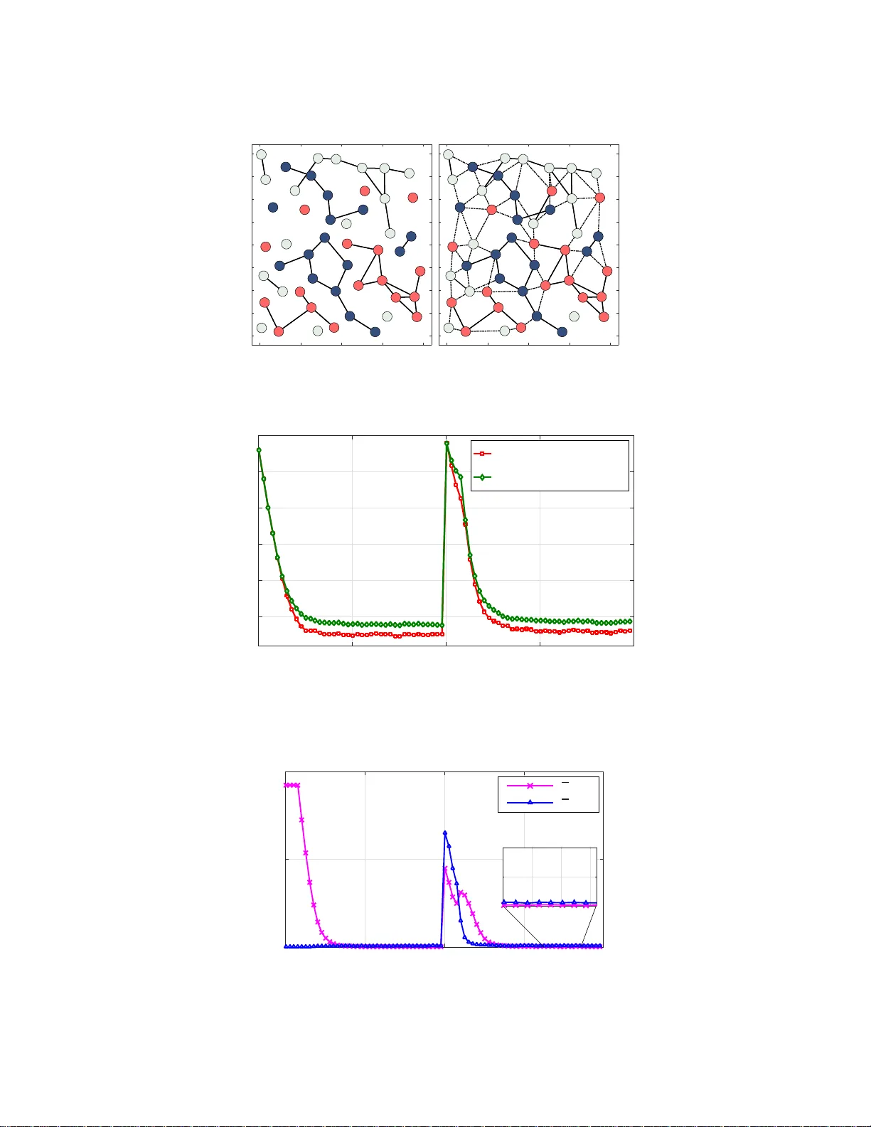
Decentralized Clustering and Linking by Networked Agents

Decen tralized Clustering and Linking b y Net w ork ed Agen ts Sahar Khaw atmi 1 , Ali H . Sayed 2 , and Abdelhak M. Zoubir 1 1 T e chnische Universit¨ at Darmst adt, S ignal Pr o c essing Gr oup, Darmstadt, Germany 2 University of Calif ornia, Dep artment of Ele ctric al Engine ering, L os A ngeles, U SA Octob er 7, 2016 Abstract W e c onsider the problem of decen tralized clustering and estimation over m ulti-task netw orks, where agen ts infer and trac k different mo dels of interes t . The agen ts do not know b eforehand whic h mo del is generating their o wn data. They also do not kn o w which agents in their neigh b orho o d b elong to the same cluster. W e prop ose a decen tralized clustering algorithm aimed at identi fying and fo rming clusters of agents of similar ob jectiv es, and at guiding coop eration to enhance th e inference p erformance. One key feature of t he proposed technique is th e integration of t he learning and clustering tasks into a single strategy . W e analyze the p erformance of the procedure and sho w that t he error probabilities of typ es I and I I decay exp onentiall y to zero with the step-size parameter. While links betw een agents follo wing different ob jectives are ignored in the clustering p rocess, we nevertheless show how to exploit these links to relay critical informa t ion across the net work for enhanced performance. Simulation results illustrate the p erformance of the proposed method in comparison to oth er useful techniques. 1 In tro d uction and Rel ated W ork Distributed learning is a p ow er ful technique for extra cting infor ma tion from net worked ag e n ts (see, e.g., [2–8] a nd the re ferences therein). In this w or k, we consider a net work of agent s connected by a g raph. Each agent senses data ge nerated by some u nknown mo del. It is assumed that there are clusters of agents within the net work, w he r e agent s in the same cluster observe data arising fr om the s ame model. How ever, the agen ts do not know whic h mo del is gener a ting their own data. They also do not know which agents in their neigh b or ho o d b elong to the same cluster. Scena r ios of this type a rise, for e x ample, in tracking applications when a collection of netw o rked agents is tasked with tracking several moving ob jects [9 – 11]. Clusters end up being formed within the netw ork with different clusters following different targets. The quality of the tracking/estimation perfor mance will b e improv ed if neighboring ag e n ts following the same target know o f each other to pro mote co op eration. It is not only coop era tion within clusters that is useful, but also co op eratio n across clusters, especia lly when ta rgets mov e in forma tio n and the lo cation of the ta rgets are correlated. Motiv ated by these considerations, the main ob jective of this work is to develop a distributed techn ique that e na bles agents to recog nize neighbor s from the same cluster and pr omotes co op era tion for improv ed inference perfor mance. There hav e b een several useful works in the literatur e on the solution of inference pro blems for such m ulti- task net works, i.e., for net works with m ultiple unkno wn mo dels (also calle d tasks) — see, e.g., [5, 12–19] and the references therein. I n the so lutions dev elo ped in [17–19], clustering is achiev e d by relying on adaptiv e combination stra tegies, whereby weigh ts on edg es b etw een a gents are ada pted and their size b ecomes smaller for unrelated ta sks. In these e a rlier w or ks, there still exists the possibility that v alid links betw een agents belo nging to the same cluster may be ov erlo oked, mainly due to erro rs during the adaptation pro cess. A mor e robust clustering metho d was pro po sed in [20] where the clustering and lear ning op er ations were de c o upled from each o ther. In this w ay , tracking e r rors do not influence the clustering mechanism a nd the resulting distributed algorithm enables the agents to identify their clusters a nd to attain improv e d learning accur acy . The work [2 0] ev aluated the err or probabilities of types I and I I, i.e., of false alarm and mis-detection for their pro po sed s cheme and s how ed that these err ors decay exp onentially with the step-size. This means that, under their scheme, the probability of correct clustering can b e made ar bitrarily close to one by selecting sufficiently small step-sizes. Still, it is preferable to mer ge the cluster ing and lea rning mechanisms rather than hav e them run separa tely of each other. Doing so r educes the computationa l burden and, if successful, can a lso lead to enhancement The work of Ali. H. Say ed was supp orted in part by NSF grants ECCS–1407712 and CCF–1524250. An early short ve r sion of this work appeared in the conference publication [1]. Thi s article has b een submitted for publication. 1 in clus ter ing acc ur acy relative to the earlie r approaches [17 – 19]. W e show e d in preliminary work [1] that this is indeed poss ible for a par ticular class of inference pro ble ms inv olving mean-squar e-erro r r isks. In this work, we g eneralize the results and devise an inte gr ate d clustering-learning appr oach for general- purp ose risk functions. Additionally , and motiv ated b y the res ults fro m [14] on adaptiv e decision-making b y net worked agents, we further incorp ora te a s mo othing mec hanism in to our str ategy to enhance the belief that agen ts hav e ab out their clusters . W e also show how to exploit the unused links a mong neighbor ing agents b elo ng ing to different clusters to r elay us eful information among ag ent s . W e carr y out a detailed a nalysis o f the resulting framework, and illustrate its super ior per formance b y means of computer s imulations. The or ganization of the w or k is a s follows. The net work and data mo del a re describ ed in Section II, while the integrated clus tering and inference fra mework is develop ed in Section I II. The net work error recursions are derived in Section IV, a nd the pro ba bilities of erro neous dec ision are derived in Section V. In Section VI we illustrate the linking tec hnique for relaying informatio n, a nd present simulation r e s ults in Sectio n VI I. Notation . W e use low e r case letters to denote vectors, upp ercas e letters for matrices, plain letters for deterministic v ar iables, a nd b oldface letters for random v ar iables. The s uper script ◦ is used to indicate true v alues. The letter E denotes the exp ectation op erator . The Euclidean norm is denoted by k · k . The symbols 1 and I denote the all- o ne vector and the identit y matrix of a ppropriate siz e s , resp ectively . W e write ( · ) ⊺ , ( · ) − 1 , and T r( · ) to denote tr a nsp osition, matrix inv e rsion, a nd matrix trace, resp ectively . T he diag {·} opera tor extracts the diago nal entries of its matrix argument and s ta cks them into a column. The k − th row (column) of matrix X is denoted by [ X ] k, : ([ X ] : ,k ). 2 Net w ork and Data Mo del 2.1 Net work Overview W e cons ider a netw or k with N agents connected b y a gra ph. It is assumed that there ar e C cluster s, denoted by C 1 , C 2 , . . . , C C , where each C m represents the set of agent indices in that cluster . W e ass o ciate an unknown column vector of size M × 1 with each cluster, deno ted by w ◦ C m ∈ R M . The aggr egation of a ll these unknowns is denoted b y w ◦ C , co l { w ◦ C 1 , w ◦ C 2 , . . . , w ◦ C C } , ( C M × 1) . (1) Each agent k wishes to recov er the model for its cluster; the unkno wn mo del for agent k is denoted b y { w ◦ k } . Obviously , this mo del ag rees with the mo del of the cluster that k b elong s to, i.e., w ◦ k = w ◦ C m if k ∈ C m . W e stack all { w ◦ k } in to a column v ecto r: w ◦ , co l { w ◦ 1 , w ◦ 2 , . . . , w ◦ N } , ( N M × 1) . (2) Figure 1 illustrates a net work with C = 3 cluster s repr esented by thre e c olors. All a gents in the same cluster are interested in estimating the s ame parameter vector. W e denote the set of neigh b o r s of an age nt k by N k . O bserve in this example that the neighbors of ag e n t k belo ng to different clusters. The clus ter information is not known to the ag ent s b eforehand. F o r instance, agent k would not know tha t its ne ig hbors are sens ing da ta arising from different mo dels . If we a llow the netw or k to p erfor m indiscriminate co o p e ration, then p erformance will degra de significant ly . F o r this reason, a cluster ing op era tion is needed to allow the agents to le arn whic h neighbor s to co op erate with tow a rds the same ob jective. The technique develop ed in this w o rk will allow agents to emphasize links to neighbor s in the s ame cluster and to disregard links to neighbor s fro m other clusters. The outcome would be a g raph structure similar to the one shown in the b ottom part of the same figure, where un warranted links are shown in dotted lines. In this way , the int er ference caused by different ob jectiv e s is av oided and the overall perfor mance for each cluster will b e improv ed. T urning off a link b etw een t wo agents means that there is no more shar ing of data b etw een them. Still, w e will explo it these “un us ed” links b y assigning to them a useful role in r elaying information a cross the net work. 2.2 T op ology Matrices In preparation for the des cription o f the prop osed strategy , we introduce the N × N adjacency ma trix Y = [ y ℓk ], whose elements are either zero or one dep ending on whether agents ar e linked by an edge or not. 2 (a) (b) Figure 1: ( T op ) Example of a netw ork topology inv olving th ree clusters, represented by three different colors. ( Bottom ) Clustered topology th at will result for the netw ork shown on top . Spec ific a lly , y ℓk = ( 1 , ℓ ∈ N k , 0 , otherwise . (3) W e as s ume that each agent k belo ngs to its neighborho o d set, k ∈ N k . The set N − k excludes k . Agents know their neigh b or ho o ds but they do not know which s ubs et o f their neighbors is sub jected to data from the same model. In order to devise a pro c edure that allows a gents to arrive at this infor mation, we introduce a second N × N clustering matrix, denoted by E i at time i , in a manner similar to the adjacency matrix Y , except tha t the v alue at location ( ℓ, k ) will b e s e t to one if agent k b elieves at time i that its neig hbo r ℓ belo ngs to the sa me cluster: e ℓk ( i ) = ( 1 , if ℓ ∈ N k and k b elieves that w ◦ k = w ◦ ℓ , 0 , otherwise . (4) The e n tr ies of E i will b e learned o nline. At every time i , we c an then use these en trie s to infer which neighbors of k are b elieved to b elong to the same cluster as k ; thes e would be the indices o f the nonzer o ent r ies in the k − th co lumn of E i . W e co llect these indices into the neighborho o d set, N k,i ; this set is a subset of N k and it evolv es ov er time during the learning pro cess. A t an y time i , ag ent k will o nly be co o pe rating with the neigh b or s within N k,i . W e will describ e in the sequel how E i is learned. 2.3 Problem F orm ulation W e asso ciate with each ag ent k a s trongly-co nv ex and differ e n tia ble risk function J k ( w k ), with a uniq ue minim um at w ◦ k . In genera l, each r isk J k ( w k ) : R M → R , is defined a s the exp ectation of some loss function Q k ( · ), say , J k ( w k ) = E Q k ( w k ; z k ) (5) 3 where z k denotes ra ndom data sensed by agent k and the exp ectation is o ver the distribution of this data. The netw o rk o f ag ents is interested in estimating the minimizers of the following aggr egate cost o ver the vectors { w k } : J glob ( w 1 , w 2 , . . . , w N ) , N X k =1 J k ( w k ) . (6) Since agents fr om different clusters do no t share the same minimizers, the aggregate cost can be re-written as J glob ( w C 1 , . . . , w C C ) , C X m =1 X k ∈C m J k ( w k ) (7) where w ◦ k = w ◦ C m . W e collect the gradient vectors o f the risk functions a cross the netw or k into the agg regate vector ∇ J ( w ) , c ol {∇ J 1 ( w 1 ) , . . . , ∇ J N ( w N ) } . (8) These g radients will not b e av ailable in mos t cases since the distribution of the data is not kno wn to enable ev a luation of the expec tation of the loss functions. In sto chastic-gr adient implement ations, it is customary to replace the ab ov e aggregate v ector by the following approximation where the true gra dient s of the risk functions are replaced by d ∇ J ( w ) , col { d ∇ J 1 ( w 1 ) , . . . , [ ∇ J N ( w N ) } (9) where each d ∇ J k ( w k ) is constructed from the gr adient of the respective loss function d ∇ J k ( w k ) = ∇ Q k ( w k ; z k ) (10) ev a luated at the co rresp onding da ta po int , z k . 2.4 Assumptions W e list here the assumptions that ar e ne e de d to drive the analysis. Thes e assumptions are typical in the analysis of sto chastic-gradient algorithms, and most of them are automatically satisfied by importa nt cases of in ter est, suc h as when the risk functions are quadratic or logistic — see, e.g ., [3, 20]. W e th us assume that ea ch individual cost function J k ( w k ) is t wice- differentiable and τ k − strongly con- vex [3, 21, 22], for some τ k > 0 . W e also require the gr adient vector of J k ( w k ) to be ζ k − Lipschitz, i.e., k∇ J k ( w k 1 ) − ∇ J k ( w k 2 ) k ≤ ζ k k w k 1 − w k 2 k (11) for an y w k 1 , w k 2 ∈ R M . Thus, the Hessian matrix function ∇ 2 J k ( w k ) is b ounded by τ k I M ≤ ∇ 2 J k ( w k ) ≤ ζ k I M (12) where τ k ≤ ζ k . E ach Hessian matrix function is a lso assumed to sa tisfy the Lipschitz condition: k∇ 2 J k ( w k 1 ) − ∇ 2 J k ( w k 2 ) k ≤ κ k k w k 1 − w k 2 k (13) for some κ k ≥ 0 and an y w k 1 , w k 2 ∈ R M . T he net work g radient noise is denoted b y s i ( w i − 1 ) which is the random pro cess defined b y s i ( w i − 1 ) , col { s 1 ,i ( w 1 ,i − 1 ) , . . . , s N ,i ( w N ,i − 1 ) } (14) where the gradient noise at agen t k a t time i is given by s k,i ( w k,i − 1 ) , d ∇ J k ( w k,i − 1 ) − ∇ J k ( w k,i − 1 ) . (15) Here we are denoting the iterates w in boldface no tation to indicate that they will actually b e sto chastic v a r iables due to the appr oximation of the true gradients. W e let { F k,i ; i ≥ 0 } denote the filtration that collects all informa tio n up to time i . W e then denote the conditional cov ariance ma trix of s k,i ( w k,i − 1 ) b y R k,i ( w k,i − 1 ) , E h s k,i ( w k,i − 1 ) s ⊺ k,i ( w k,i − 1 ) | F k,i − 1 i . (16) It is a ssumed that the g radient noise pro cess satisfies the follo wing prop erties for an y w k,i − 1 in F k,i − 1 [3]: 4 1.Martingale difference [3 , 2 0]: E [ s k,i ( w k,i − 1 ) | F k,i − 1 ] = 0 (17) 2.Bounded fourth-order momen t [3, 20]: E  k s k,i ( w k,i − 1 ) k 4 | F k,i − 1  ≤ β 2 k k w ◦ k − w k,i − 1 k 4 + ρ 4 k (18) for some β 2 k , ρ 4 k ≥ 0 . 3.Lipsc hitz conditional cov aria nce function [3, 20]: k R k,i ( w ◦ k ) − R k,i ( w k,i − 1 ) k ≤ θ k k w ◦ k − w k,i − 1 k η k (19) for some θ k ≥ 0 and 0 < η k ≤ 4 . 4.Con vergent conditional cov ariance matr ix [3, 20]: R k , lim i →∞ R k,i ( w ◦ k ) > 0 (20) where R k is symmetric and p os itive definite. 2.5 Data Mo del W e assume tha t each agent k runs a n indep endent stochastic gr adient-descen t algorithm of the form: ψ k,i = ψ k,i − 1 − µ k d ∇ J k ( ψ k,i − 1 ) (21) where µ k > 0 is a sma ll step-size par ameter, and ψ k,i denotes the intermediate estimate for w ◦ k at time i . Co op eration among agents will b e limited to neighbor s that b elong to the same cluster. Therefor e, follo wing the up date (21), ideally , agen t k sho uld only share data with agent ℓ if w ◦ k = w ◦ ℓ . The a gents do not know which agents in their neighborho o d b elong to the sa me clus ter ; this infor mation is le a rned in r eal-time. Therefore, agent k will only share data with ag e nt ℓ if it b elieves that w ◦ k = w ◦ ℓ . Sp ecifically , ag ent k w ill combine the estimates from its neig hbors in a con vex manner as follows: w k,i = N X ℓ =1 a ℓk ( i ) ψ ℓ,i (22) where the nonnegative combination co efficients { a ℓk ( i ) } satisfy a kk ( i ) > 0 , a ℓk ( i ) = 0 for ℓ / ∈ N k,i , N X ℓ =1 a ℓk ( i ) = 1 . (23) In the next section, we explain ho w the combin ation co e fficien ts { a ℓk ( i ) } are selected in order to p erform the comb ined tasks o f estimation and clustering . 3 Clustering Sc heme Let δ > 0 denote the smallest distance among the cluster mo dels, { w ◦ C m } . F or a n y distinct a, b ∈ { 1 , . . . , C } , it then holds that k w ◦ C a − w ◦ C b k ≥ δ. (24) W e introduce an N × N trus t matr ix F i ; ea ch en try f ℓk ( i ) ∈ [0 , 1] of this matrix reflects the amount of trust that agent k has in neighbor ℓ ∈ N − k belo nging to its cluster. The entries { f ℓk ( i ) } are constructed as follows. Agent k first co mputes the Bo ole a n v aria ble: b ℓk ( i ) = ( 1 , if k ψ ℓ,i − w k,i − 1 k 2 ≤ α, 0 , otherwise (25) 5 where α is a thres hold v alue. The trust lev el f ℓk ( i ) is smoothed as follows: f ℓk ( i ) = ν f ℓk ( i − 1 ) + (1 − ν ) b ℓk ( i ) (26) where the forg etting factor, 0 < ν < 1, determines the sp eed with which trust in neighbor ℓ accumulates ov er time. Once f ℓk ( i ) exceeds so me threshold γ , agent k decla r es that neighbor ℓ belongs to its cluster and sets the corresp onding en try e ℓk ( i ) in matr ix E i to the v alue one: e ℓk ( i ) = ( 1 , if f ℓk ( i ) ≥ γ , 0 , otherwise (27) where 0 < γ < 1. F or completeness, we set for any agent k , b kk ( i ) = f kk ( i ) = e kk ( i ) = 1 . Obser ve that the c o mputation of the binary v aria ble b ℓk ( i ) couples the ψ and w v ar iables. Therefor e , b y using smo o thed v a lues { f ℓk ( i ) } for the trust v aria bles , w e are able to co uple the clustering and inference pro cedures int o a single iterative algor ithm rather than run them s eparately . The smo o thing reduces the influence of erroneo us clustering decisions on the infere nce task. The following listing summar izes the pro po sed strategy . Algorithm 1 (Distributed clustering scheme) Initialize F − 1 = B − 1 = E − 1 = I and ψ − 1 = w − 1 = 0. for i ≥ 0 do for k = 1 , . . . , N do ψ k,i = ψ k,i − 1 − µ k d ∇ J k ( ψ k,i − 1 ) (28) for ℓ ∈ N − k do b ℓk ( i ) = ( 1 , if k ψ ℓ,i − w k,i − 1 k 2 ≤ α 0 , otherwise (29) f ℓk ( i ) = ν f ℓk ( i − 1 ) + (1 − ν ) b ℓk ( i ) (30) upda te e ℓk ( i ) according to (2 7 ) end for select { a ℓk ( i ) } according to (23 ) and set w k,i = N X ℓ =1 a ℓk ( i ) ψ ℓ,i (31) end for end for 4 Mean-Square-Error Analysis W e no w examine the mean-square perfor mance o f the propo s ed scheme. W e collect the estimates from across the net work into the blo ck vectors: ψ i , co l { ψ 1 ,i , ψ 2 ,i , . . . , ψ N ,i } , (32) w i , co l { w 1 ,i , w 2 ,i , . . . , w N ,i } , (33) and define the matr ices A i , A i ⊗ I M , M , diag { µ 1 , . . . , µ N } ⊗ I M . (34) where A i = [ a ℓk ( i )]. F ro m (2 1 ) w e find that the net work vector ψ i evolv es o ver time according to ψ i = ψ i − 1 − M∇ J ( ψ i − 1 ) − M s i ( ψ i − 1 ) (35) 6 where ∇ J ( · ) and s i ( · ) are defined in (8) and (14). Likewise, from (22) w e find that w i = A ⊺ i ψ i . (36) T o pr o ceed, w e introduce the error v ecto rs e ψ k,i , w ◦ k − ψ k,i , e w k,i , w ◦ k − w k,i , (37) and collect them from acr oss the netw o rk in to e ψ i , co l { e ψ 1 ,i , . . . , e ψ N ,i } , (38) e w i , co l { e w 1 ,i , . . . , e w N ,i } . (39) W e further define the net work mean-squa r e deviation (MSD) b efore and after the fusion step at the time i by MSD ψ ( i ) , E k e ψ i k 2 , (40) MSD w ( i ) , E k e w i k 2 . (41) 4.1 Error Dynamics Appea ling to the mea n-v a lue theorem [3 , p. 3 2 7] w e can write ∇ J ( ψ i − 1 ) = − H i − 1 e ψ i − 1 (42) where H i − 1 , diag { H k,i − 1 } N k =1 (43) and eac h matrix H k,i − 1 is given by H k,i − 1 , Z 1 0 ∇ 2 J k ( w ◦ k − t e ψ k,i − 1 ) dt. (44) Substituting (42) in to (35) yields ψ i = ψ i − 1 + M H i − 1 e ψ i − 1 − M s i ( ψ i − 1 ) . (45) By subtracting w ◦ defined in (2) fro m b oth sides, we get e ψ i = ( I N M − M H i − 1 ) e ψ i − 1 + M s i ( ψ i − 1 ) (46) which means that the error r ecursion for eac h individual agent k is giv en b y e ψ k,i = ( I M − µ k H k,i − 1 ) e ψ k,i − 1 + µ k s k,i ( ψ k,i − 1 ) . (47) It is a rgued in [3, p. 34 7] that for step-sizes µ k satisfying 0 < µ k < 2 τ k ζ 2 k + β 2 k (48) the mean-square- error quantit y E k e ψ k,i k 2 conv erg es exp onentially ac cording to the recur sion: E k e ψ k,i k 2 ≤ ξ k E k e ψ k,i − 1 k 2 + µ 2 k ρ 2 k (49) where 0 ≤ ξ k < 1 and is giv en by ξ k = 1 − 2 µ k τ k + µ 2 k ( ζ 2 k + β 2 k ) . (50) 7 It is further shown in [3, pp. 352, 378] that for small step-sizes s atisfying (48), the error rec ur sion (46) ha s bo unded first, second, a nd fourth-order momen ts in the following sense: lim sup i →∞ k E e ψ i k = O ( µ max ) (51) lim sup i →∞ E k e ψ i k 2 = O ( µ max ) (52) lim sup i →∞ E k e ψ i k 4 = O ( µ 2 max ) (53) where µ max is the maxim um step-size acros s all agent s. W e further intro duce the co nstant blo ck diago nal matr ix: H , diag { H 1 , . . . , H N } , H k , ∇ 2 J k ( w ◦ k ) , (54) and replace (46) by the approximate r ecursion e ψ ′ i = ( I N M − MH ) e ψ ′ i − 1 + M s i ( ψ i − 1 ) (55) where the random matrix H i − 1 is re pla ced by H . It was also shown in [3, pp. 38 2, 384 ] that, for sufficien tly small step-sizes, the error iterates tha t are generated b y this recur sion s atisfy: lim i →∞ E e ψ ′ i = 0 (56) lim sup i →∞ E k e ψ ′ i k 2 = O ( µ max ) (57) lim sup i →∞ E k e ψ i − e ψ ′ i k 2 = O ( µ 2 max ) (58) lim sup i →∞ E k e ψ ′ i k 2 = lim sup i →∞ E k e ψ i k 2 + O ( µ 3 / 2 max ) . (59) These results imply that, for lar ge enough i , the er rors e ψ and e ψ ′ are close to each other in the mea n-square- error sense. 4.2 One Useful Prop erty The ab ov e construction guarantees one useful prop erty if the clustering pro ces s do es not incur err ors of type II, meaning that links that should be disc o nnected are indeed disconnec ted. This implies that w ◦ ℓ = w ◦ k whenever a ℓk ( i ) > 0. Using (23), it follows that N X ℓ =1 a ℓk ( i ) w ◦ ℓ = w ◦ k (60) or, equiv ale n tly , A ⊺ i w ◦ = w ◦ . (61) Subtracting w ◦ from both sides of (36) yields, w ◦ − w i = w ◦ − A ⊺ i ψ i . (62) Using (61) w e rewrite (62) as: e w i = A ⊺ i e ψ i . (63) T aking the blo ck maximum norm [23, p. 435] of b oth sides and using the sub-m ultiplica tive prop er ty of norms implies that k e w i k b, ∞ ≤ k A ⊺ i k b, ∞ k e ψ i k b, ∞ = k e ψ i k b, ∞ (64) since A i is left-stochastic and, therefore, k A ⊺ i k b, ∞ = 1 . It follows that E k e w i k b, ∞ ≤ E k e ψ i k b, ∞ . (65) Results (64) and (65) ensur e that the size of the error in the w domain is b ounded b y the size of the error in the ψ doma in if there are no errors of type I I during clustering. 8 5 P erformance Analysis W e are ready to examine the b ehavior o f the probabilities of e r roneous decis ions of t yp es I and I I for ea ch agent k , namely , the probabilities that a link b etw een k and one of its neighbors will b e either erro neously disconnected (when it s ho uld be connec ted) or erroneo usly co nnec ted (when it should b e disconnected): Type-I: w ◦ ℓ = w ◦ k and a ℓk ( i ) = 0 , (66) Type-I I: w ◦ ℓ 6 = w ◦ k and a ℓk ( i ) 6 = 0 (67) for an y ℓ ∈ N k . After long enough i , these probabilities are deno ted resp ectively by: P I = P r ( f ℓk ( i ) < γ | w ◦ ℓ = w ◦ k ) , (68) P II = P r ( f ℓk ( i ) ≥ γ | w ◦ ℓ 6 = w ◦ k ) . (69) Assessing the proba bilities (68 ) and (6 9) is a challenging ta s k and needs to b e purs ued under s ome simplifying conditions to facilitate the analysis. This is due to the sto chastic nature of the clustering and learning pro cesses, and due to the coupling amo ng the agents. Our purp ose is to provide insights into the p erforma nce of these pro cess es after sufficien t learning time has elapsed. The analysis that follows adjusts the approa ch of [14] to the current setting. Different from [14] where there were only tw o mo dels and all agents were tr ying to co nv erge to one of these tw o models, w e now ha ve a m ultitude of clusters and agents that are trying to conv erg e to their o wn cluster mo del. 5.1 Smo othing Pro cess In order to determine bo unds for P I and P II we study the pr obability distribution o f the trust v aria ble f ℓk ( i ). W e ha ve from (26) that: f ℓk ( i ) = ν i +1 f ℓk ( − 1) + (1 − ν ) i X j =0 ν j b ℓk ( i − j ) (70) where b ℓk ( i ) is modelled as a Bernoulli random v ariable with success probability p : b ℓk ( i ) = ( 1 , with probability p, 0 , with probability (1 − p ) . (71) W e alr eady know from (49) that, after sufficient time, the iterates ψ k,i conv erg e to the tr ue mo dels w ◦ k in the mean-squar e-erro r sense. Hence, it is rea sonable to assume that the v a lue of p b ecomes la r gely time-inv ariant and corresp onds to the pr obability of the ev ent des crib ed b y k ψ ℓ,i − w k,i − 1 k 2 ≤ α, for large i. (72) W e denote the proba bilities of tr ue and false as signments b y P d = P r ( b ℓk ( i ) = 1 | w ◦ ℓ = w ◦ k ) , (73) P f = P r ( b ℓk ( i ) = 1 | w ◦ ℓ 6 = w ◦ k ) . (74) These probabilities also satisfy: (1 − P d ) = Pr ( k ψ ℓ,i − w k,i − 1 k 2 > α | w ◦ ℓ = w ◦ k ) , (75) P f = P r ( k ψ ℓ,i − w k,i − 1 k 2 ≤ α | w ◦ ℓ 6 = w ◦ k ) . (76) After sufficient iter ations, the influence of the initia l condition in (70) can b e ig nored and we ca n appr oximate f ℓk ( i ) b y the following ra ndom ge o metric series: f ℓk ( i ) ≈ (1 − ν ) i X j =0 ν j b ℓk ( i − j ) . (77) 9 As explained in [14], althoug h it is gener ally not true, we ca n simplify the analysis by assuming that, fo r large enough i , the ra ndom v aria bles { b ℓk ( m ) } in (7 7 ) are independent and iden tica lly distributed. This assumption is motiv ated by the fact that the models o bserved by the different cluster s are assumed to be sufficiently distinct from each other by virtue of (24). Now, recall tha t Mar ko v’s inequality [2 4, p. 47] implies that for an y nonnegative random v ariable x and po sitive scala r u , it holds that: Pr ( x ≥ u ) = P r ( x 2 ≥ u 2 ) ≤ E x 2 u 2 . (78 ) T o apply (78) to the v ar iable f ℓk ( i ), w e need to determine its second-or de r momen t. F or this purp os e , we follow [14] and in tro duce the change of v aria ble : b ◦ ℓk ( i − j ) , b ℓk ( i − j ) − p p p (1 − p ) . (79) It can b e v er ified that the v aria bles { b ◦ ℓk ( m ) } are i.i.d. with zero mean and unit v a riance. As a res ult, we rewrite (77) for la rge i as: f ℓk ( i ) ≈ p + p p (1 − p ) f ◦ ℓk ( i ) (80) where f ◦ ℓk ( i ) , (1 − ν ) i X j =0 ν j b ◦ ℓk ( i − j ) (81) has zero mean a nd its v ar iance is g iven b y V ar [ f ◦ ℓk ( i )] = E  f ◦ ℓk ( i )  2 − h E f ◦ ℓk ( i ) i 2 = 1 − ν 1 + ν (1 − ν 2( i +1) ) ≈ 1 − ν 1 + ν . (82) Returning to (68) we no w hav e, with p re placed b y P d : P I ≈ P r ( f ℓk ( i ) < γ | w ◦ ℓ = w ◦ k ) ≤ P r  | f ◦ ℓk ( i ) | > P d − γ p P d (1 − P d )     w ◦ ℓ = w ◦ k  ≤ 1 − ν 1 + ν · P d (1 − P d ) ( P d − γ ) 2 (83) where we applied (78) and the fact that, for any t wo generic ev ents B 1 and B 2 , if B 1 implies B 2 , then the probability of ev ent B 1 is less than the probability of event B 2 [25]. Similarly , by r eplacing p by P f , we obtain P II ≤ 1 − ν 1 + ν · P f (1 − P f ) ( γ − P f ) 2 . (84) In expressio ns (83) and (84), it is assumed that the size of the threshold v a lue γ used in (27) sa tis fie s γ < P d and γ > P f . Since we usually desire the pro ba bilit y of false alar m to b e sma ll and the proba bilit y of detection to b e close to one, these conditions can be met by γ ∈ (0 , 1). W e sho w in the next s ection that this is indeed the case. Results (83) a nd (8 4) provide b ounds o n the proba bilities o f er rors I and I I. W e next establish that P d → 1 and P f → 0 to conclude that P I → 0 and P II → 0. 5.2 The Distribution of t he V ariables After sufficient iter ations and for small enough step-s izes, it is known that e ach ψ ℓ,i exhibits a distribution that is ne a rly Gaussian [26–31]: ψ ℓ,i ∼ N ( w ◦ ℓ , µ ℓ Γ ℓ ) (85) 10 where the matrix Γ ℓ is symmetric, p ositive semi-definite, and the solution to the follo wing Lyapuno v equa- tion [26]: H ℓ Γ ℓ + Γ ℓ H ℓ = R ℓ (86) where the Hessian matr ix H ℓ is defined by (54) and R ℓ is the steady-state cov aria nce matrix o f the gradient noise at a gent ℓ defined b y (20). W e next in tro duce the v e c to r ¯ w ◦ k,i , N X ℓ =1 a ℓk ( i ) w ◦ ℓ . (87) which sho uld be compare d with expressio n (22). The vector (8 7) is the r e s ult of fusing the actual mo dels using the same combination weigh ts av ailable at time i . It follows tha t w k,i exhibits a distribution that is near ly Gaussia n since the iterates { ψ ℓ,i } can be as s umed to b e indep endent of each other due to the decoupled nature of their up dates : w k,i ∼ N ( ¯ w ◦ k,i , Ω k,i ) (88) where Ω k,i is symmetric, pos itive semi-definite, and given b y Ω k,i , N X ℓ =1 µ ℓ a 2 ℓk ( i )Γ ℓ . (89) Let g ℓk,i , ψ ℓ,i − w k,i − 1 (90) and note that g ℓk,i is again approximately Gaussian distributed with g ℓk,i ∼ N ( ¯ g i , ∆ ℓk,i ) (91) where ¯ g i , w ◦ ℓ − ¯ w ◦ k,i − 1 (92) and ∆ ℓk,i is symmetric, p os itive semi-definite, and b ounded b y (in view of Jensen’s inequalit y [3, p. 769] 2 ): ∆ ℓk,i ≤ 2  µ ℓ Γ ℓ + Ω k,i − 1  . (93) F rom (89), (93 ) and for any ℓ and k it holds tha t: ∆ ℓk,i = O ( µ max ) . (94) 5.3 The Statistics of k g ℓk ,i k 2 W e now examine the statistics of the main test v aria ble for our algorithm from (25), namely , k g ℓk,i k 2 . Let { A k,i − 1 ; i > 0 } denote the filtration that collects all { a ℓk ( i − 1) } infor mation up to time i − 1. Then, note that E  k g ℓk,i k 2 | A k,i − 1  = E h T r  g ℓk,i g ⊺ ℓk,i    A k,i − 1 i = k ¯ g i k 2 + T r ( ∆ ℓk,i ) . (95) 2 Since E ( a + b ) 2 ≤ 2 E a 2 + 2 E b 2 . 11 Since g ℓk,i is Gaussian, it ho lds that E  k g ℓk,i k 4 | A k,i − 1  = E  k g ℓk,i − ¯ g i + ¯ g i k 4 | A k,i − 1  = E h  k g ℓk,i − ¯ g i k 2 + 2( g ℓk,i − ¯ g i ) ⊺ ¯ g i + k ¯ g i k 2  2   A k,i − 1 i = E  k g ℓk,i − ¯ g i k 4 | A k,i − 1  + 2 E  k g ℓk,i − ¯ g i k 2 k ¯ g i k 2 | A k,i − 1  + k ¯ g i k 4 + 4 ¯ g ⊺ i E  ( g ℓk,i − ¯ g i )( g ℓk,i − ¯ g i ) ⊺ | A k,i − 1  ¯ g i = E  k g ℓk,i − ¯ g i k 4 | A k,i − 1  + 2 T r ( ∆ ℓk,i ) k ¯ g i k 2 + k ¯ g i k 4 + 4 k ¯ g i k 2 ∆ ℓk,i (96) where all odd order moment s o f ( g ℓk,i − ¯ g i ) are zero. Likewise,  E  k g ℓk,i k 2 | A k,i − 1   2 =  E  k g ℓk,i − ¯ g i + ¯ g i k 2 | A k,i − 1   2 =  E  k g ℓk,i − ¯ g i k 2 | A k,i − 1  + k ¯ g i k 2  2 = [ T r ( ∆ ℓk,i ) ] 2 + 2 T r ( ∆ ℓk,i ) k ¯ g i k 2 + k ¯ g i k 4 . (97) According to Lemma A.2 of [32, p. 11], w e hav e E  k g ℓk,i − ¯ g i k 4 | A k,i − 1  = [ T r ( ∆ ℓk,i ) ] 2 + 2 T r ( ∆ 2 ℓk,i ) . (98) Using (96) and (98), the v a riance of k g ℓk,i k 2 is given by V ar  k g ℓk,i k 2 | A k,i − 1  = 4 k ¯ g i k 2 ∆ ℓk,i + 2 T r ( ∆ 2 ℓk,i ) . (99) Note from (95) that the mean of k g ℓk,i k 2 is dominated by k ¯ g i k 2 for sufficien tly small step-sizes. It follows from the Cheb yshev’s inequality [3 3, p. 455 ] that: Pr    k g ℓk,i k 2 − E  k g ℓk,i k 2 | A k,i − 1    ≥ u     A k,i − 1  ≤ V ar  k g ℓk,i k 2 | A k,i − 1  u 2 = O ( µ max ) (10 0) for any constant u > 0, which implies that the v ariance of k g ℓk,i k 2 is in the or der of µ max . Therefo re, when w ◦ ℓ = w ◦ k the probability mass o f k g ℓk,i k 2 will concentrate around E ( k g ℓk,i k 2 ), whic h is in the order of O ( µ max ) ≈ 0. On the other hand, when w ◦ ℓ 6 = w ◦ k , the probabilit y mass of k g ℓk,i k 2 will co ncent rate aro und E ( k g ℓk,i k 2 ) ≈ k ¯ g i k 2 > 0 . Obviously the threshold should b e c hosen a s: 0 < α < δ 2 , where δ is the clustering resolution. 5.4 Error Probabilities It is seen fro m (75) a nd (76) that 1 − P d corres p o nds to the rig h t tail probability of k g ℓk,i k 2 when w ◦ ℓ = w ◦ k , and P f corres p o nds to the left tail probability of k g ℓk,i k 2 when w ◦ ℓ 6 = w ◦ k . T o examine these probabilities, we follow arguments similar to [20] a nd apply them to the cur r ent con text. W e in tr o duce the eigen-decomp ositio n ∆ ℓk,i = U i Λ i U ⊺ i (101) 12 where U i is or thonormal a nd Λ i is diagonal and nonnegative-definite. W e further in tr o duce the normalized v a r iables: x i , Λ − 1 / 2 i U ⊺ i g ℓk,i , (102) ¯ x i , Λ − 1 / 2 i U ⊺ i ¯ g i (103) and it fo llows from (91), (102) , and (103) that x i ∼ N ( ¯ x i , I M ) . (104) Note also from (10 2) that k g ℓk,i k 2 = x ⊺ i Λ i x i = M X h =1 λ h,i x 2 h,i . ( 1 05) where x h,i denotes the h − th element of x i and λ h,i denotes the h − th diag onal elemen t of Λ i . 5.4.1 The probabilit y 1 − P d It follows from the inequalit y k g ℓk,i k 2 = x ⊺ i Λ i x i ≤ k ∆ ℓk,i k · k x i k 2 , (106) that the follo wing relation is satisfied {k g ℓk,i k 2 > α } ⊆ { k ∆ ℓk,i k · k x i k 2 > α } . (107) Defining α k ( i ) , α/ k ∆ ℓk,i k (108) , w e can write using (107): Pr ( k g ℓk,i k 2 > α | w ◦ ℓ = w ◦ k ) ≤ Pr ( k x i k 2 > α k ( i ) | ¯ x i = 0 ) . (109) W e kno w from (104) that k x i k 2 ∼ X 2 M (110) where X 2 M denotes the Chi-squar e distribution with M deg rees o f freedom and its mean v alue is M . According to the Cher noff bo und for the central Chi- square distribution with M degr ees o f free dom 3 we hav e Pr  k x i k 2 > α k ( i )   ¯ x i = 0  = P r  k x i k 2 > M · α k ( i ) M     ¯ x i = 0  ≤ exp h − M 2  α k ( i ) M − log  1 + α k ( i ) M − 1 i =  α k ( i ) · e M  M / 2 · exp h − α k ( i ) 2 i (111) where e is Euler’s num b er. F or small enough step-sizes w e conclude fro m (94 ), (108), and (111) tha t after sufficient itera tio ns, it holds that: (1 − P d ) ≤ O ( e − c 1 /µ max ) (112) for some constan t c 1 > 0 . 3 Let y ∼ X 2 r . Aco ording to the Chernoff b ound for the cen tral Chi-square distribution with r degrees of fr eedom, for an y ǫ > 0 it holds that [34, p. 2501]: Pr ( y > r (1 + ǫ )) ≤ exp [ − r 2 ( ǫ − log(1 + ǫ ))]. 13 5.4.2 The probabilit y P f The approximate characteristic function of k g ℓk,i k 2 [20, Eq. (118)] when w ◦ ℓ 6 = w ◦ k is giv en by: c k g ℓk,i k 2 ( t ) ≈ e j t k w ◦ ℓ − w ◦ k k 2 − 2 t 2 k w ◦ ℓ − w ◦ k k 2 Λ i (113) which implies that for sufficien tly small µ max , k g ℓk,i k 2 ∼ N ( k w ◦ ℓ − w ◦ k k 2 , 4 k w ◦ ℓ − w ◦ k k 2 Λ i ) . (114) Therefore, from [20] 4 we obtain that Pr ( k g ℓk,i k 2 < α | w ◦ ℓ 6 = w ◦ k ) ≈ Q  k w ◦ ℓ − w ◦ k k 2 − α 2 k w ◦ ℓ − w ◦ k k Λ i  ≤ 1 2 exp  − ( k w ◦ ℓ − w ◦ k k 2 − α ) 2 8 k w ◦ ℓ − w ◦ k k 2 Λ i  (115) where the letter Q refer s here to the traditional Q − function (the tail probability of the s ta ndard Gaussian distribution). F or small enough step-sizes, after s ufficie nt iter ations and from (94), (1 01), and (115), it holds that P f ≤ O ( e − c 2 /µ max ) (11 6) for some constant c 2 > 0. It is then seen that the probabilities P I and P II are exp ected to appro ach zero exp onentially fast for v a nishing step-sizes. 6 Linking Application 6.1 Clustering With Linking Sc heme W e prop ose in this section an additional mechanism to enhance the p erformance o f each cluster by using the unused links to relay information. Figur e 2 s hows the linked topo logy that results for the same example shown earlie r in Fig. 1(b). The figure shows that the links which are suppos ed to be unused for sharing data among neighbors belong ing to different clusters, are used now to r e lay data among ag ents. W e assume in this section that the links among agents a re symmetric , i.e. if ℓ ∈ N k ⇐ ⇒ k ∈ N ℓ . Under normal oper ation, each agent k will be receiving and pro cessing iterates only from those neighbors that it belie ves b elong to the same cluster a s k . W e mo dify this operatio n by allowing k to receive iterates fr o m al l of its neigh b ors. It will con tinue to use the iterates from neigh b o r s in the sa me cluster to up date its weigh t estimate w k,i . The itera tes that arrive from neighbors that may b elong to other clusters ar e no t used dur ing this fusio n pro cess . Instead, they will b e r elay ed forw a rd b y a gent k as follows. F or each o f its neighbor s ℓ ∈ N k , agent k will s end ψ k,i and another vector φ kℓ,i The vector φ kℓ,i is constructed as follows. Agent k chooses from amo ng all the iterates it receives from its neigh b or s, that iterate that is closest to ψ ℓ,i : φ kℓ,i = arg min k ψ m,i − ψ ℓ,i k 2 . { k,m } ∀ m ∈N k , m / ∈N ℓ (117) Observe that the minimization is o ver k and a ll neig hbo rs of k that are not neighbors o f ℓ . This condition is imp ortant to avoid receiving the sa me information m ultiple times. O bserve also that under this scheme, agent k will need to receive the iterates from a ll of its neighbors (those that it believes b elong to its clus ters and those that do not); it also nee ds to receive informa tion ab out their neighborho o ds , i.e., the N ℓ for each of its ne ig hbors ℓ . 4 Let y ∼ N (0 , 1). Acoording to the Chernoff b ound for the Gaussian error function it holds that [35]: Q ( y ) ≤ 1 2 exp [ − y 2 2 ]. 14 Figure 2: The clustered and linked top ology th at will result for the netw ork show n in Fig. 1. The b old d ashed lines depict the links u sed for relaying data among agen ts. The following steps describ e the clus tering with linking algor ithm. W e collect all { φ ℓk,i } in to a matr ix Φ i . By setting γ = 0 . 5 in Eq. (27) the op era tion of s e tting each en try e ℓk ( i ) b ecomes rounding to the neares t int eg er and is deno ted b y ⌊·⌉ . Algorithm 2 (Clustering with link ing s cheme) Initialize F − 1 = B − 1 = E = I , Φ − 1 = 0 , and ψ − 1 = w − 1 = 0. for i ≥ 0 do for k = 1 , . . . , N do ψ k,i = ψ k,i − 1 − µ k d ∇ J k ( ψ k,i − 1 ) (118) for ℓ ∈ N − k do send ψ k,i and φ kℓ,i − 1 receive ψ ℓ,i and φ ℓk,i − 1 b ℓk ( i ) = ( 1 , if k φ ℓk,i − 1 − w k,i − 1 k 2 ≤ α 0 , otherwise (119) f ℓk ( i ) = ν f ℓk ( i − 1 ) + (1 − ν ) b ℓk ( i ) (120) e ℓk ( i ) = ⌊ f ℓk ( i ) ⌉ (121) end for select { a ℓk ( i ) } according to (23) and set w k,i = N X ℓ =1 a ℓk ( i ) φ ℓk,i − 1 (122) upda te { φ kℓ ( i ) } according to (11 7) end for end for 7 Sim ulation Results W e consider a fully co nnected netw ork with 50 randomly dis tributed agents. The age n ts observe data originating fro m three differen t models ( C = 3). Each model w ◦ C m ∈ R M × 1 is gener a ted as follo ws: w ◦ C m = 15 5 10 15 20 25 30 35 40 45 50 1.5 2 2.5 No de index, k (b) 5 10 15 20 25 30 35 40 45 50 0.1 0.2 0.3 (a) σ 2 v,k T r( R u,k ) Figure 3: The statistical noise and sig n al profi les o ver the netw ork. (a) (b) Figure 4: The n etw ork topology (a) and the clustered topology at steady-state (b ). [ w r 1 , . . . , w r M ] ⊺ , with e n tr ies w r c ∈ [1 , − 1 ]. In o ur example we set M = 2; lar g er v alues of M are g enerally easier for clustering and, ther efore, w e illustr ate the o pe r ation of the algorithm for M = 2. The assignment of the agents to mo de ls is random. Agents having the same colo r b elong to the same cluster. The maximum nu mber of neighbors is n max = 6. Every agent k has acc ess to a scala r measurement d k ( i ) a nd a 1 × M regres s ion vector u k,i . The measurements acro ss the agents are assumed to b e generated via the linea r regres s ion mo del d k ( i ) = u k,i w ◦ k + v k ( i ), where v k ( i ) is meas ur ement no ise assumed to b e a zero-mea n white r andom pro c ess that is independent over space. It is also as sumed that the regressio n data u k,i is independent ov er space and indep endent of v ℓ ( j ) for all k, ℓ , i, j . All r a ndom pro c esses are a s sumed to be stationary . The statistical pr ofile of the noise across the age nts for k = 1 , . . . , N is shown in Fig. 3(a). The reg ressor s are of s ize M = 2 and hav e diago nal cov ariance matrices R u,k shown in Fig. 3(b). W e set { µ, α, ν, δ, γ } = { 0 . 0 5 , 0 . 015 , 0 . 98 , 0 . 17 , 0 . 5 } . W e use the unifor m combination p olicy to gener ate the co efficients { a ℓk ( i ) } . Figure 4(a) sho w s the top olog y of one of 100 Monte Ca rlo expe riments. Figure 4(b) presents the fina l top ology after applying the clustering tec hnique. Figur e 5(a) depicts the sim ulated transient mea n-square deviation (MSD) of the net work compared to other clustering methods . The model assignments change at time instan t i = 400 . 16 Time, i 0 200 400 600 800 MSD (dB) -30 -25 -20 -15 -10 -5 simulated [20] simulated [19] simulated (MS D) Figure 5: The transien t mean- square dev iation (MSD) using different approac h es. 0 100 200 300 400 500 600 700 800 0 0.25 0.5 Ti me , i (b) 0 100 200 300 400 500 600 700 800 0 0.25 0.5 (a) [19] scheme [20] scheme prop osed scheme v I v II Figure 6: The n ormalized clustering errors of types I and II o ver the netw ork. The normalized clustering errors of types I and II by each a gent k a t time i ar e giv e n, resp ectively , by v I ,k ( i ) , ( 1 − [ E i ] : ,k ) ⊺ × ([ E ◦ ] : ,k − [ E i ] : ,k ) ( n k − 1) (123) v II ,k ( i ) , [ E i ] ⊺ : ,k × ([ E i ] : ,k − [ E ◦ ] : ,k ) ( n k − 1) (124) where E ◦ is the true clustering matrix. Figur es 6(a)–6 (b) depict the normalized clustering errors v I and v II ov er the net work. Using the same setup of the previous example, Fig. 7(a) shows the top ology of one exper imen t with the clustering tec hnique only . Figure 7(b) presents the fina l topo logy when we apply the clustering with linking techn ique. Figur e 8 indicates the sim ulated transie nt mean-square deviation (MSD) of the agents with and without the linking technique. The no r malized clustering er rors ov er the netw ork are shown in Fig. 9. 8 Conclusion W e prop osed a distributed algorithm that carr ies o ut the tasks of estimation and clustering simultaneously with expo nentially decaying error pr o babilities for false decisions. W e show ed how the a gents c ho o se the subset of their neighbors to co op er ate with a nd tur n off suspicious links. The simulations illustrate the 17 (a) (b) Figure 7: The clustered netw ork topology at steady-state (a) and the clustered and linke d topology at steady-state (b). Time, i 0 200 400 600 800 MSD (dB) -25 -20 -15 -10 -5 0 clusterin g with li nking clusterin g without linki ng Figure 8: The t ransien t mean-square deviation with and without applying the linking technique. Time, i 0 200 400 600 800 Clustering error 0 0.2 0.4 0 0.025 0.05 v I v II Figure 9: The n ormalized clustering errors of types I and II o ver the netw ork. 18 per formance of the prop o s ed strategy and compare with other re la ted works. W e prop osed an additional step to enhance the p erfor mance b y link ing , a s m uch as po ssible, the agents that b elong ing to the same cluster and do no t hav e dir e ct link s to connect them. References [1] S. K haw atmi, A. M. Zoubir, and A. H. Say ed. Decentralized cluster ing over adaptive netw orks . In Pr o c. 23r d Eu r op e an Signal Pr o c essing Confer enc e ( EUSIPCO) , pages 2745– 2749 , Nice, F rance, September 2015. [2] A. H. Say ed. Adaptive netw o rks. In Pr o c. IEEE , volume 102, pag es 460–497 , April 2014. [3] A. H. Sa yed. Adaptation, lear ning, and optimization over net works. F ound. T r ends in Mach. L e arn. , 7(4–5):31 1–80 1 , July 2014 . [4] J. B. P redd, S. B. Kulk arni, and H. V. Poor . Distr ibuted learning in wire le ss s ensor net works. IEEE Signal Pr o c essing Ma gazine , 23(4):56–69 , July 2006. [5] A. Bertra nd and M. Mo onen. Distributed ada ptive no de- sp ecific signal estimation in fully connected sensor netw or ks, Pa rt I: Sequential no de updating . IEEE T r ans. Signal Pr o c essing , 58(10 ):5277– 5291, Octob er 2010. [6] S. Cho uv a rdas, K. Slav a kis, a nd S. Theo dor idis . Adaptiv e robust distributed learning in diffusion sensor net works. IEEE T ra ns . Signal Pr o c essing , 59(10 ):4692– 4707, 2011. [7] A. Nedic a nd A. O zdaglar . Distributed subgradient metho ds for m ultia gent optimiza tio n. IEEE T r ans. Autom. Contr ol , 54(1):4 8–61, J anuary 2009. [8] S. Al-Say ed, A. M. Zoubir, a nd A. H Say ed. Robust adaptation in impulsive noise. IEEE T r ans. on Signal Pr o c essing , 64(11 ):2 851–2 865, 2 016. [9] J. Liu, M. Ch u, and J. E. Reich. Multitar get tracking in distributed sensor netw orks . IEEE Signal Pr o c essing Mag. , 24(3):36–46 , 2007. [10] X. Zhang. Adaptive co nt r ol and reconfigur ation o f mobile wireless sensor netw ork s for dynamic m ulti- target trac k ing. IEEE T r ans. A u tom. Contr ol , 56(10 ):2429– 2444, 2011. [11] M. Z. Lin, M. N. Murthi, and K. Premar atne. Mobile adaptiv e net works for pursuing m ultiple targ e ts. In Pr o c. IEEE Intern ational Confer enc e on A c oust., Sp e e ch, and Signal Pr o c essing (ICASSP) , pa ges 3217 – 3221, South Brisbane, QLD, Apr. 2015. [12] I. F rancis a nd S. Chatterjee. Classification and estimation of several multiple regr essions. The Annals of Statistics , 2(3):55 8–56 1 , 1974. [13] L. Jacob, F. Bach, and J.-P . V ert. Cluster ed multi-task lear ning: A conv ex formulation. In Pr o c. N eur al Inform. Pr o c essing Systems. (NIPS) , pages 1–8, V anco uver, Canada , December 20 08. [14] S. Y. T u and A. H. Say ed. Distributed decision-making ov er adaptive netw o rks. IEEE T r ans. Signal Pr o c essing , 62 (5):1054– 1069 , March 2014 . [15] J. Chen, C. Richard, and A. H. Sayed. Multitask diffusion a da ptation ov er net works. IEEE T r ans. Signal Pr o c essing , 62(16 ):4 129–4 144, August 20 14. [16] N. Bo gdanovic, J . Plata- Chav es, and K. Berb eridis. Distributed diffusion-based LMS for no de-sp ecific parameter estimation ov er adaptive netowrks. In Pr o c. IEEE International Confer enc e on A c oust ., Sp e e ch, and S ignal Pr o c essing (ICASSP) , pages 7 223–7 227, Florence, Italy , Ma y 2014. [17] X. Z hao a nd A. H. Say ed. Clustering via diffusion adaptation over net works. In Pr o c. International Workshop on Co gnitive Inform. Pr o c essing (CIP) , page s 1–6 , Baio na, Spain, May 2012. 19 [18] J. Chen, C. Richard, and A. H. Say ed. Diffusion LMS ov er mult ita sk netw orks. IEEE T ra n s. Signal Pr o c essing , 63 (11):2733 –274 8 , June 2015 . [19] J. Chen, C. Richard, and A. H. Sa yed. Adaptive clustering for multitask diffusion netw orks. In Pr o c. 23r d Eur op e an Signal Pr o c essing Confer enc e (EUSIPCO) , pages 200– 204, Nice, F rance, Se ptember 20 15. [20] X. Zhao and A. H. Say ed. Distributed clustering and learning over netw orks. IEE E T r ans. Signal Pr o c essing , 63 (13):3285 –330 0 , July 2015. [21] D. Bertsek as. Convex A n alysis and Optimization . Athena Scientific, 2003. [22] S. Boyd and L. V anden b erg he. Convex Optimizatio n . Camb r idge Univ er sity Press, 2004. [23] A. H. Say ed. Diffusion adaptation ov er netw orks. In R. Chellapa and S. Theo doridis , editors , A c ademic Pr ess Libr ary in Signal Pr o c essing , volume 3, pages 323–45 4. Academic Press, Elsevier, 2014. [24] O. Knill. Pr ob ability The ory and Sto chastic Pr o c esses with Applic ations . O verseas Pres s India Priv ate Limited, 2009. [25] A. Pap oulis and S. U. Pillai. Pr ob ability, R andom V ariables, and Sto chastic Pr o c esses . McGraw-Hill Higher Education, 2002. [26] J. Chen and A. H. Say e d. On the pro bability distribution o f distributed optimiza tion s trategies. In Pr o c. Glob al Confe re n c e on Signal and Information Pr o c essing (Glob alSIP) , pa g es 5 55–5 58, Austin, TX, Decem be r 20 13. [27] J. Chen and A. H. Say ed. On the limiting b ehavior o f distr ibuted optimization strategies. In Pr o c. 50th Annual Al lerton Confer enc e on Communic ation, Contr ol, and Computing , pages 153 5–154 2, Mo nt icello, IL, October 201 2. [28] X. Zhao a nd A. H. Say ed. Pr obability distribution o f s tea dy-state error s a nd adaptation ov er netw or ks. In Pr o c. IEEE Statistic al Signal Pr o c essing Worksho p (SS P) , pa ges 253–25 6, Nice, F r ance, June 2011. [29] J. Sacks. Asymptotic distribution of sto chastic a pproximation pr o cedures. The Annals of Mathematic al Statistics , 29(2):373– 4 05, June 1958. [30] M. B. Nevelson a nd R. Z. Hasminskii. Sto chastic a pproximation and recurs ive estimation. A m eric an Mathematic al So ciety , 19 76. [31] R. Bitmead. Conv e r gence in distribution of LMS- t y pe adaptive para meter estimates . IEEE T r ans. Autom. Contr ol , 28(1):5 4–60, J anuary 1983. [32] A. H. Say ed. A daptive Filters . Wiley , NJ, 2008. [33] B. F ristedt and L. Gr ay . A Mo dern Appr o ach t o Pr ob ability The ory . Birkhauser , Bos to n, MA, 19 97. [34] P . L i, T. J. Hastie, and K. W. Ch ur ch. Nonlinear estimators and ta il bo unds for dimension reductio n in ℓ 1 using Cauc hy random pro jections. J. Mach. L e arn. Res. , 8:2 4 97–2 5 32, Octob er 2007. [35] M. Chiani, D. Darda ri, and M. K. Simon. New exponential b ounds a nd approximations for the compu- tation of e r ror pr obability in fading ch a nnels. IEE E T r ans. on W ir eless Communic ations , 2(4):84 0–84 5 , July 2003. 20