Demystifying ResNet

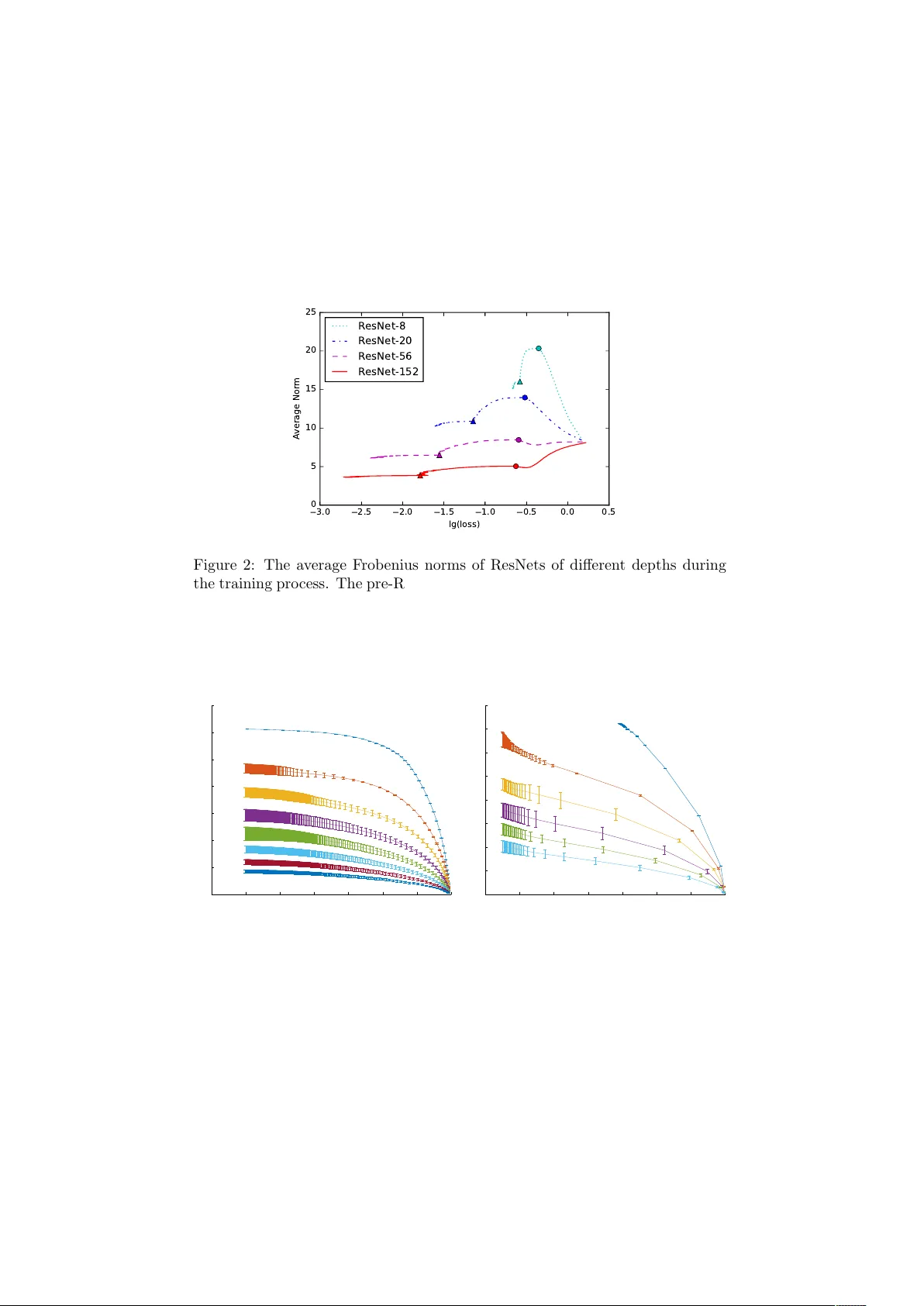
Dem ystifying ResNet Sihan Li 1 , Jian tao Jiao 2 , Y anjun Han 2 , and Tsac hy W eissman 2 1 Tsingh ua Universit y 2 Stanford Univ ersity Ma y 23, 2017 Abstract The Residual Net work (ResNet), prop osed in He et al. (2015a), uti- lized shortcut connections to significantly reduce the difficult y of training, whic h resulted in great performance b oosts in terms of both training and generalization error. It was empirically observed in He et al. (2015a) that stacking more la yers of residual blo cks with shortcut 2 results in smaller training error, while it is not true for shortcut of length 1 or 3. W e provide a theoretical explanation for the uniqueness of shortcut 2. W e show that with or without nonlinearities, by adding shortcuts that ha ve depth tw o, the condition num b er of the Hessian of the loss function at the zero initial p oin t is depth-inv arian t, whic h makes training v ery deep mo dels no more difficult than shallo w ones. Shortcuts of higher depth result in an extremely flat (high-order) stationary p oint initially , from which the optimization algorithm is hard to escape. The shortcut 1, ho wev er, is essentially equiv alent to no shortcuts, whic h has a condition n umber explo ding to infinity as the n umber of la yers grows. W e further argue that as the num b er of la yers tends to infinit y , it suffices to only lo ok at the loss function at the zero initial p oint. Extensiv e exp eriments are provided accompanying our theoretical re- sults. W e sho w that initializing the netw ork to small w eights with shortcut 2 ac hieves significantly b etter results than random Gaussian (Xavier) ini- tialization, orthogonal initialization, and shortcuts of deep er depth, from v arious p erspectives ranging from final loss, learning dynamics and sta- bilit y , to the b ehavior of the Hessian along the learning pro cess. 1 In tro duction Residual netw ork (ResNet) w as first prop osed in He et al. (2015a) and extended in He et al. (2016). It follo w ed a principled approach to add shortcut connections ev ery tw o lay ers to a V GG-style netw ork (Simony an and Zisserman, 2014). The new netw ork b ecomes easier to train, and achiev es b oth low er training and test errors. Using the new structure, He et al. (2015a) managed to train a net work with 1001 lay ers, whic h was virtually imp ossible b efore. Unlike High wa y Net work (Sriv astav a et al., 2015a,b) which not only has shortcut paths but also b orro ws the idea of gates from LSTM (Sainath et al., 2015), ResNet do es not 1 ha ve gates. Later He et al. (2016) found that b y k eeping a clean shortcut path, residual netw orks will p erform even b etter. Man y attempts hav e been made to impro ve ResNet to a further exten t. “ResNet in ResNet” (T arg et al., 2016) adds more con v olution la yers and data paths to eac h la yer, making it capable of represen ting sev eral types of residual units. “ResNets of ResNets” (Zhang et al., 2016) construct multi-lev el short- cut connections, which means there exist shortcuts that skip multiple residual units. Wide Residual Net works (Zagoruyko and Komo dakis, 2016) makes the residual netw ork shorter but wider, and achiev es state of the art results on sev- eral datasets while using a shallow er net work. Moreov er, some existing mo dels are also rep orted to b e impro ved by shortcut connections, including Inception- v4 (Szegedy et al., 2016), in which shortcut connections make the deep netw ork easier to train. Understanding why the shortcut connections in ResNet could help reduce the training difficult y is an imp ortan t question. Indeed, He et al. (2015a) suggests that lay ers in residual netw orks are learning residual mappings, making them easier to represent identit y mappings, which preven ts the netw orks from degra- dation when the depths of the netw orks increase. Ho wev er, V eit et al. (2016) claims that ResNets are actually ensem bles of shallo w netw orks, which means they do not solve the problem of training deep net works completely . In Hardt and Ma (2016), they sho wed that for deep linear residual netw orks with shortcut 1 does not hav e spurious lo cal minim um, and analyzed and experimented with a new ResNet architecture with shortcut 2. W e would lik e to emphasize that it is not true that ev ery type of identit y mapping and shortcut works. Quoting He et al. (2015a): “But if F has only a single layer, Eqn.(1) is similar to a line ar layer: y = W 1 x + x , for which we have not observe d advantages.” “De ep er non-b ottlene ck R esNets (e.g., Fig. 5 left) also gain ac cur acy fr om incr e ase d depth (as shown on CIF AR-10), but ar e not as e c onomic al as the b ottlene ck R esNets. So the usage of b ottlene ck designs is mainly due to pr ac- tic al c onsider ations. We further note that the de gr adation pr oblem of plain nets is also witnesse d for the b ottlene ck designs. ” Their empirical observ ations are inspiring. First, the shortcut 1 mentioned in the first paragraph do not work. It clearly contradicts the theory in Hardt and Ma (2016), which forces us to conclude that the nonlinear netw ork b e- ha ves essentially in a differen t manner from the linear netw ork. Second, noting that the non-b ottlene ck ResNets hav e shortcut 2, but the b ottleneck ResNets use shortcut 3, one sees that shortcuts with depth three also do not ease the optimization difficulties. In ligh t of these empirical observ ations, it is sensible to sa y that a reasonable theoretical explanation m ust b e able to distinguish shortcut 2 from shortcuts of other depths, and clearly demonstrate wh y shortcut 2 is sp ecial and is able to ease the optimization pro cess so significantly for deep mo dels, while shortcuts of other depths ma y not do the job. Moreo ver, analyzing deep linear mo dels ma y not b e able to provide the righ t intuitions. 2 2 Main results W e provide a theoretical explanation for the unique role of shortcut of length 2. Our arguments can be decomposed in to t w o parts. 1. F or very deep (general) ResNet, it suffices to initialize the weigh ts at zero and searc h lo cally: in other words, there exist a global minimum whose w eight functions for each lay er hav e v anishing norm as the num b er of la yers tends to infinity . 2. F or very deep (general) ResNet, the loss function at the zero initial p oint exhibits radically different b eha vior for shortcuts of differen t lengths. In particular, the Hessian at the zero initial p oin t for the 1-shortcut netw ork has condition num b er growing un b oundedly when the num b er of lay ers gro ws, while the 2-shortcut netw ork enjoys a depth-inv arian t condition n umber. ResNet with shortcut length larger than 2 has the zero initial p oin t as a high order saddle p oint (with Hessian a zero matrix), which ma y be difficult to escape from in general. W e pro vide extensive exp erimen ts v alidating our theoretical argumen ts. It is mathematically surprising to us that although the deep linear residual netw orks with shortcut 1 has no spurious lo cal minim um (Hardt and Ma, 2016), this result do es not generalize to the nonlinear case and the training difficulty is not reduced. Deep residual netw ork of shortcut length 2 admits spurious local minim um in general (suc h as the zero initial point), but pro v es to w ork in practice. As a side pro duct, our exp eriments reveal that ortho gonal initialization (Saxe et al., 2013) is sub optimal . Although b etter than Xavier initialization (Glorot and Bengio, 2010), the initial condition num bers of the net works still explo de as the netw orks become deep er, which means the netw orks are still initialized on “bad” submanifolds that are hard to optimize using gradien t descen t. 3 Mo del W e first generalize a linear netw ork by adding shortcuts to it to mak e it a line ar r esidual network . W e organize the netw ork in to R r esidual units . The r -th residual unit consists of L r la yers whose weigh ts are W r, 1 , . . . , W r,L r − 1 , denoted as the tr ansformation p ath , as well as a shortcut S r connecting from the first lay er to the last one, denoted as the shortcut p ath . The input-output mapping can be written as y = R Y r =1 ( L r − 1 Y l =1 W r,l + S r ) x = W x, (1) where x ∈ R d x , y ∈ R d y , W ∈ R d y × d x . Here if b ≥ a , Q b i = a W i denotes W b W ( b − 1) · · · W ( a +1) W a , otherwise it denotes an iden tity mapping. The matrix W represents the com bination of all the linear transformations in the net work. Note that by setting all the shortcuts to zeros, the netw ork will go back to a ( P r ( L r − 1) + 1)-la yer plain linear net work. Instead of analyzing the general form, w e concentrate on a sp ecial kind of linear residual net works, where all the residual units are the same. 3 Definition 1. A linear residual netw ork is called an n -shortcut line ar network if 1. its lay ers ha ve the same dimension (so that d x = d y ); 2. its shortcuts are identit y matrices; 3. its shortcuts ha ve the same depth n . The input-output mapping for suc h a net work b ecomes y = R Y r =1 ( n Y l =1 W r,l + I d x ) x = W x, (2) where W r,l ∈ R d x × d x . Then we add some activ ation functions to the netw orks. W e concentrate on the case where activ ation functions are on the transformation paths, which is also the case in the latest ResNet (He et al., 2016). Definition 2. An n -shortcut linear netw ork b ecomes an n -shortcut network if elemen t-wise activ ation functions σ pre ( x ) , σ mid ( x ) , σ post ( x ) are added at the transformation paths, where on a transformation path, σ pre ( x ) is added b e- fore the first weigh t matrix, σ mid ( x ) is added b etw een tw o weigh t matrices and σ post ( x ) is added after the last w eigh t matrix. pr e mid pos t Figure 1: An example of differen t position for nonlinearities in a residual unit of a 2-shortcut netw ork. Note that n -shortcut linear net works are sp ecial cases of n -shortcut net works, where all the activ ation functions are identit y mappings. 4 Theoretical study 4.1 Small w eigh ts prop ert y of (near) global minim um ResNet uses MSRA initialization (He et al., 2015b). It is a kind of scaled Gaussian initialization that tries to keep the v ariances of signals along a trans- formation path, which is also the idea behind Xa vier initialization (Glorot and Bengio, 2010). How ever, b ecause of the shortcut paths, the output v ariance of the entire netw ork will actually explo de as the netw ork becomes deep er. Batch normalization units partly solved this problem in ResNet, but still they cannot prev ent the large output v ariance in a deep netw ork. A simple idea is to zero initialize all the w eigh ts, so that the output v ariances of residual units sta y the same along the netw ork. It is worth noting that as found in He et al. (2015a), the deep er ResNet has smaller magnitudes of lay er resp onses. This phenomenon has b een confirmed in our exp eriments. As illus- trated in Figure 2 and Figure 3, the deep er a residual netw ork is, the small its 4 a verage F rob enius norm of weigh t matrices is, both during the training pro cess and when the training ends. Also, Hardt and Ma (2016) prov es that if all the w eight matrices hav e small norms, a linear residual netw ork with shortcut of length 1 will hav e no critical p oints other than the global optim um. 3.0 2.5 2.0 1.5 1.0 0.5 0.0 0.5 lg(loss) 0 5 10 15 20 25 Average Norm ResNet-8 ResNet-20 ResNet-56 ResNet-152 Figure 2: The a verage F robenius norms of ResNets of different depths during the training pr o cess. The pre-ResNet implemen tation in https://github.com/ facebook/fb.resnet.torch is used. The learning rate is initialized to 0.1, decreased to 0.01 at the 81 st ep och (marked with circles) and decreased to 0.001 at the 122 nd ep och (marked with triangles). Each mo del is trained for 200 ep o chs. -3.5 -3 -2.5 -2 -1.5 -1 -0.5 0 log 10 (loss - loss opt ) 0 0.5 1 1.5 2 2.5 3 3.5 Average Norm depth = 2 depth = 4 depth = 8 depth = 16 depth = 32 depth = 64 depth = 128 depth = 256 -1.4 -1.2 -1 -0.8 -0.6 -0.4 -0.2 0 log 10 (loss) 0 0.5 1 1.5 2 2.5 3 3.5 4 Average Norm depth = 2 depth = 4 depth = 8 depth = 16 depth = 32 depth = 64 Figure 3: The a verage F robenius norms of 2-shortcut netw orks of differen t depths during the training pro cess when zero initialized. Left : Without non- linearities. Righ t : With ReLUs at mid p ositions. All these evidences indicate that zero is sp ecial in a residual netw ork: as the net work b ecomes deeper, the training tends to end up around it. Th us, we are lo oking into the Hessian at zero. As the zero is a saddle p oin t, in our exp eriments w e use zero initialization with small random perturbations to escap e from it. W e first Xa vier initialize the weigh t matrices, and then multiply a small constant (0 . 01) to them. 5 No w we presen t a simplified ResNet structure with shortcut of length 2, and pro ve that as the residual net work b ecomes deep er, there exists a solution whose weigh t functions hav e v anishing norm, which is observed in ResNet as we men tioned. This argumen t is motiv ated by Hardt and Ma (2016). W e concentrate on a sp ecial kind of netw ork whose o verall transformation can b e written as y = R Y r =1 ( W r, 2 ReLU( W r, 1 x + b r ) + I d x ) , (3) where b r ∈ R d x is the bias term. It can seen as a simplified version of ResNet (He et al., 2016). Note that although this net work is not a 2-shortcut net work, its Hessian still follo w the form of Theorem 2, th us its condition num b er is still depth-in v arian t. W e will also mak e some assumptions on the training samples. Assumption 1. Assume n ≥ 3 , m  1 , for every 1 ≤ µ ≤ m , k x µ k 2 = 1 , y µ ∈ { e 1 , · · · , e d y } wher e { e 1 , · · · , e d y } ar e d y standar d b asis ve ctors in R d y . The formats of training samples describ e ab o ve are common in practice, where the input data are whitened and the lab els are one-hot enco ded. F ur- thermore, we b orrow an mild assumption from Hardt and Ma (2016) that there exists a minim um distance b et ween every t wo data points. Definition 3. The minimum distance of a group of v ectors is defined as d min ( a 1 , a 2 , · · · , a m ) = min 1 ≤ i 400), only ResNets with shortcut 2 gain adv antages from the growth of depth, where other netw orks suffer from degradation as the net work b ecomes deep er. References Chris Bishop. Exact calculation of the hessian matrix for the multila yer p er- ceptron, 1992. 11 0 100 200 300 400 500 600 Depth 5 6 7 8 9 10 11 12 13 Test Error / % Training Result on CIFAR-10 1-shortcut 2-shortcut 3-shortcut 4-shortcut Figure 9: CIF AR-10 results of ResNets with different depths and shortcut depths. Means and standard deviations are estimated based on 10 runs. ResNets with a shortcut depth larger than 4 yield w orse results and are omitted in the figure. Y ann N Dauphin, Razv an Pascan u, Caglar Gulcehre, Kyunghyun Cho, Surya Ganguli, and Y oshua Bengio. Identifying and attac king the saddle point problem in high-dimensional non-con vex optimization. In A dvanc es in neur al information pr o c essing systems , pages 2933–2941, 2014. Rong Ge, F urong Huang, Chi Jin, and Y ang Y uan. Escaping from saddle p oin tsonline stochastic gradient for tensor decomp osition. In Pr o c e e dings of The 28th Confer enc e on L e arning The ory , pages 797–842, 2015. Xa vier Glorot and Y oshua Bengio. Understanding the difficult y of training deep feedforw ard neural netw orks. In Aistats , volume 9, pages 249–256, 2010. Rob ert M Gray . T o eplitz and cir culant matric es: A r eview . now publishers inc, 2006. Moritz Hardt and T engyu Ma. Identit y matters in deep learning. arXiv pr eprint arXiv:1611.04231 , 2016. Kaiming He, Xiangyu Zhang, Shao qing Ren, and Jian Sun. Deep residual learn- ing for image recognition. arXiv pr eprint arXiv:1512.03385 , 2015a. Kaiming He, Xiangyu Zhang, Shao qing Ren, and Jian Sun. Delving deep in to rectifiers: Surpassing h uman-level p erformance on imagenet classification. In Pr o c e e dings of the IEEE International Confer enc e on Computer Vision , pages 1026–1034, 2015b. Kaiming He, Xiangyu Zhang, Shao qing Ren, and Jian Sun. Iden tity mappings in deep residual netw orks. arXiv pr eprint arXiv:1603.05027 , 2016. Vino d Nair and Geoffrey E Hin ton. Rectified linear units improv e restricted b oltzmann machines. In Pr o c e e dings of the 27th International Confer enc e on Machine L e arning (ICML-10) , pages 807–814, 2010. 12 T ara N Sainath, Oriol Vin yals, Andrew Senior, and Ha¸ sim Sak. Con volutional, long short-term memory , fully connected dee p neural netw orks. In A c oustics, Sp e e ch and Signal Pr o c essing (ICASSP), 2015 IEEE International Confer enc e on , pages 4580–4584. IEEE, 2015. Andrew M Saxe, James L McClelland, and Surya Ganguli. Exact solutions to the nonlinear dynamics of learning in deep linear neural netw orks. arXiv pr eprint arXiv:1312.6120 , 2013. Karen Simony an and Andrew Zisserman. V ery deep conv olutional netw orks for large-scale image recognition. arXiv pr eprint arXiv:1409.1556 , 2014. Rup esh K Sriv asta v a, Klaus Greff, and J ¨ urgen Schmidh ub er. T raining very deep net works. In A dvanc es in neur al information pr o c essing systems , pages 2377–2385, 2015a. Rup esh Kumar Sriv astav a, Klaus Greff, and J ¨ urgen Sc hmidhuber. High wa y net works. arXiv pr eprint arXiv:1505.00387 , 2015b. Christian Szegedy , Sergey Ioffe, Vincen t V anhouck e, and Alex Alemi. Inception- v4, inception-resnet and the impact of residual connections on learning. arXiv pr eprint arXiv:1602.07261 , 2016. Sasha T arg, Diogo Almeida, and Kevin Lyman. Resnet in resnet: Generalizing residual architectures. arXiv pr eprint arXiv:1603.08029 , 2016. Andreas V eit, Michael Wilb er, and Serge Belongie. Residual netw orks are exp onen tial ensembles of relativ ely shallow net works. arXiv pr eprint arXiv:1605.06431 , 2016. Sergey Zagoruyk o and Nik os Komo dakis. Wide residual net works. arXiv pr eprint arXiv:1605.07146 , 2016. Ke Zhang, Miao Sun, T ony X Han, Xingfang Y uan, Liru Guo, and T ao Liu. Residual net works of residual net works: Multilevel residual net works. arXiv pr eprint arXiv:1608.02908 , 2016. A Pro ofs of theorems A.1 Pro of of Theorem 1 Lemma 1. Given matrix A, A 0 such that A =  a 1 · · · a i − 1 a i a i +1 · · · a m  , (11) A 0 =  a 1 · · · a i − 1 a 0 i a i +1 · · · a m  , (12) wher e a 1 , · · · , a i , · · · , a m and a 0 i ar e unit ve ctors in R d x , d min ( A ) , d min ( A ) ≥ ρ/ 2 , k a i − a 0 i k 2 = d . Ther e exists W 1 , W 2 ∈ R d x × d x , b ∈ R d x such that W 2 ReLU( W 1 A + b · 1 ) + A = A 0 , (13) k W 1 k F = k W 2 k F = √ 8 d ρ . (14) 13 Pr o of. Let W 1 = √ 8 d ρ      a T i 0 . . . 0      , (15) W 2 = p 8 /d ρ  a 0 i − a i 0 · · · 0  , (16) b = √ 8 d ρ ( ρ 2 8 − 1) , (17) It is trivial to c heck that Equation 13 and 14 hold. Lemma 1 constructs a residual unit that c hange one column of its input b y d . Now we are going to pro of that b y rep eating this step, the input matrix X can b e transfered into the output matrix Y . Lemma 2. Given that d x ≥ 3 , ther e exists a se quenc e of matrix X 0 , X 1 , · · · , X s wher e X 0 = X, X s = Y , (18) s = m d ( ρ ( m − 1) 2 + 1) π d e , (19) such that for every 1 ≤ i ≤ s , X i − 1 and X i c onform to L emma 1 with a distanc e smal ler than d . Pr o of. In order to complete the transformation, we can mo dify X column by column. F or eac h column vector, in order to mo ve it while preserving a minim um distance, we can dra w a minor arc on the unit sphere connecting the starting and the ending p oin t, bypassing eac h obstacle by a minor arc with a radius of ρ/ 2 if needed, as sho wn in Figure 10. The length of the path is smaller than ( ρ ( m − 1) 2 + 1) π , th us d ( ρ ( m − 1) 2 +1) π d e steps are sufficient to k eep eac h step shorter than d . Rep eating the pro cess for m times will give us a legal construction. Figure 10: The path of a mo ving vector that preserves a minimum distance of ρ/ 2. No w w e can prov e Theorem 1 with the all these lemmas ab o ve. 14 Pr o of of The or em 1. Using Lemma 2, we ha ve d ≥ O ( m ( ρm + 1)). Then use Lemma 1, w e can get a construction that satisfies k W r,l k F ≤ O ( r m nρ ( m + 1 ρ )) . (20) A.2 Pro of of Theorem 2 Definition 5. The elements in Hessian of an n -shortcut net w ork is defined as H ind( w 1 ) , ind( w 2 ) = ∂ 2 L ∂ w 1 ∂ w 2 , (21) where L is the loss function, and the indices ind( · ) is ordered lexicographically follo wing the four indices ( r , l , j, i ) of the weigh t v ariable w r,l i,j . In other words, the priorit y decreases along the index of shortcuts, index of w eight matrix inside shortcuts, index of column, and index of row. Note that the collection of all the weigh t v ariables in the n -shortcut netw ork is denoted as w . W e study the b ehavior of the loss function in the vicinity of w = 0 . Lemma 3. Assume that w 1 = w r 1 ,l 1 i 1 ,j 1 , · · · , w N = w r N ,l N i N ,j N ar e N p ar ameters of an n -shortcut network. If ∂ 2 L ∂ w 1 ··· ∂ w N    w = 0 is nonzer o, ther e exists r and k 1 , · · · , k n such that r k m = r and l k m = m for m = 1 , · · · , n . Pr o of. Assume there do es not exist suc h r and k 1 , · · · , k n , then for all the shortcut units r = 1 , · · · , R , there exists a w eigh t matrix l suc h that none of w 1 , · · · , w N is in W r,l , so all the transformation paths are zero, which means W = I d x . Then ∂ 2 L ∂ w 1 ··· ∂ w N    w = 0 = 0, leading to a con tradiction. Lemma 4. Assume that w 1 = w r 1 ,l 1 i 1 ,j 1 , w 2 = w r 2 ,l 2 i 2 ,j 2 , r 1 ≤ r 2 . L et L 0 ( w 1 , w 2 ) denotes the loss function with al l the p ar ameters exc ept w 1 and w 2 set to 0, w 0 1 = w 1 ,l 1 i 1 ,j 1 , w 0 2 = w 1+ 1 ( r 1 6 = r 2 ) ,l 2 i 2 ,j 2 . Then ∂ 2 L 0 ( w 1 ,w 2 ) ∂ w 1 ∂ w 2 | ( w 1 ,w 2 )= 0 = ∂ 2 L 0 ( w 0 1 ,w 0 2 ) ∂ w 0 1 ∂ w 0 2 | ( w 0 1 ,w 0 2 )= 0 . Pr o of. As all the residual units exp ect unit r 1 and r 2 are identit y transforma- tions, reordering residual units while preserving the order of units r 1 and r 2 will not affect the o verall transformation, i.e. L 0 ( w 1 , w 2 ) | w 1 = a,w 2 = b = L 0 0 ( w 0 1 , w 0 2 ) | w 0 1 = a,w 0 2 = b . So ∂ 2 L 0 ( w 1 ,w 2 ) ∂ w 1 ∂ w 2 | ( w 1 ,w 2 )= 0 = ∂ 2 L 0 ( w 0 1 ,w 0 2 ) ∂ w 0 1 ∂ w 0 2 | ( w 0 1 ,w 0 2 )= 0 . Pr o of of The or em 2. No w we can pro ve Theorem 2 with the help of the previ- ously established lemmas. 1. Using Lemma 3, for an n -shortcut netw ork, at zero, all the k -th order partial deriv atives of the loss function are zero, where k ranges from 1 to n − 1. Hence, the initial p oint zero is a ( n − 1)th-order stationary point of the loss function. 15 Residual Unit 1 Residual Unit 1 Residual Unit 2 Residual Unit 2 … … … … Figure 11: The Hessian in n = 2 case. It follo ws from Lemma 3 that only off-diagonal subblo cks in eac h diagonal block, i.e., the blo cks marked in orange (slash) and blue (c hessb oard), are non-zero. F rom Lemma 4, we conclude the translation in v ariance and that all blocks marked in orange (slash) (resp. blue (c hessb oard)) are the same. Given that the Hessian is symmetric, the blo c ks mark ed in blue and orange are transp oses of each other, and thus it can b e directly written as Equation (8). 2. Consider the Hessian in n = 2 case. Using Lemma 3 and Lemma 4, the form of Hessian can b e directly written as Equation (8), as illustrated in Figure 11. So we hav e eigs( H ) = eigs(  0 A T A 0  ) = ± q eigs( A T A ) . (22) Th us cond( H ) = p cond( A T A ), whic h is depth-inv ariant. Note that the dimension of A is d 2 x × d 2 x . T o get the expression of A , consider tw o parameters that are in the same residual unit but different weigh t matrices, i.e. w 1 = w r, 2 i 1 ,j 1 , w 2 = w r, 1 i 2 ,j 2 . If j 1 = i 2 , we hav e A ( j 1 − 1) d x + i 1 , ( j 2 − 1) d x + i 2 = ∂ 2 L ∂ w 1 ∂ w 2    w = 0 = ∂ 2 P m µ =1 1 2 m ( y µ i 1 − x µ i 1 − σ post ( w 1 σ mid ( w 2 σ pre ( x µ j 2 )))) 2 ∂ w 1 ∂ w 2    w = 0 = σ 0 mid (0) σ 0 post (0) m m X µ =1 σ pre ( x µ j 2 )( x µ i 1 − y µ i 1 ) . (23) Else, we hav e A ( j 1 − 1) d x + i 1 , ( j 2 − 1) d x + i 2 = 0. Noting that A ( j 1 − 1) d x + i 1 , ( j 2 − 1) d x + i 2 in fact only dep ends on the t wo indices i 1 , j 2 (with a small difference dep ending on whether j 1 = i 2 ), we mak e a 16 d x × d x matrix with ro ws indexed b y i 1 and columns indexed by j 2 , and the en try at ( i 1 , j 2 ) equal to A ( j 1 − 1) d x + i 1 , ( j 2 − 1) d x + i 2 . Apparently , this matrix is equal to σ 0 mid (0) σ 0 post (0)(Σ X σ pre ( X ) − Σ Y σ pre ( X ) ) when j 1 = i 2 , and equal to the zero matrix when j 1 6 = i 2 . T o simplify the expression of A , we rearrange the columns of A by a p erm utation matrix, i.e. A 0 = AP , (24) where P ij = 1 if and only if i = (( j − 1) mo d d x ) d x + d j d x e . Basically it p erm utes the i -th column of A to the j -th column. Then we hav e A = σ 0 mid (0) σ 0 post (0)    Σ X σ pre ( X ) − Σ Y σ pre ( X ) . . . Σ X σ pre ( X ) − Σ Y σ pre ( X )    P T . (25) So the eigen v alues of H b ecomes eigs( H ) = ± σ 0 mid (0) σ 0 post (0) q eigs((Σ X σ pre ( X ) − Σ Y σ pre ( X ) ) T (Σ X σ pre ( X ) − Σ Y σ pre ( X ) )) , (26) whic h leads to Equation (9). 3. No w consider the Hessian in the n = 1 case. Using Lemma 4, the form of Hessian can be directly written as Equation (10). T o get the expressions of A and B in σ pre ( x ) = σ post ( x ) = x case, consider t wo parameters that are in the same residual units, i.e. w 1 = w r, 1 i 1 ,j 1 , w 2 = w r, 1 i 2 ,j 2 . W e ha ve B ( j 1 − 1) d x + i 1 , ( j 2 − 1) d x + i 2 = ∂ 2 L ∂ w 1 ∂ w 2    w = 0 (27) = ( 1 m P m µ =1 x µ j 1 x µ j 2 i 1 = i 2 0 i 1 6 = i 2 (28) Rearrange the order of v ariables using P , w e hav e B = P    Σ X X . . . Σ X X    P T . (29) Then consider t wo parameters that are in different residual units, i.e. w 1 = w r 1 , 1 i 1 ,j 1 , w 2 = w r 2 , 1 i 2 ,j 2 , r 1 > r 2 . 17 W e ha ve A ( j 1 − 1) d x + i 1 , ( j 2 − 1) d x + i 2 = ∂ 2 L ∂ w 1 ∂ w 2    w = 0 (30) =          1 m P m µ =1 ( x µ i 1 − y µ i 1 ) x µ j 2 + x µ j 1 x µ j 2 j 1 = i 2 , i 1 = i 2 1 m P m µ =1 ( x µ i 1 − y µ i 1 ) x µ j 2 j 1 = i 2 , i 1 6 = i 2 1 m P m µ =1 x µ j 1 x µ j 2 j 1 6 = i 2 , i 1 = i 2 0 j 1 6 = i 2 , i 1 6 = i 2 (31) In the same wa y , w e can rewrite A as A =    Σ X X − Σ Y X . . . Σ X X − Σ Y X    P T + B . (32) B Exp erimen t setup on MNIST W e took the exp eriments on whitened v ersions of MNIST. T en greatest principal comp onen ts are kept for the dataset inputs. The dataset outputs are represented using one-hot encoding. The net work w as trained using gradient descent. F or ev ery ep o c h, the Hessians of the netw orks were calculated using the metho d prop osed in Bishop (1992). As the | λ | min of Hessian is usually very unstable, w e calculated | λ | max | λ | (0 . 1) to represent condition num b er instead, where | λ | (0 . 1) is the 10 th p ercen tile of the absolute v alues of eigenv alues. As pr e , mid or p ost p ositions are not defined in linear net works without shortcuts, when comparing Xavier or orthogonal initialized linear netw orks to 2-shortcut net works, we added ReLUs at the same p ositions in linear net works as in 2-shortcuts netw orks. 18