Designing labeled graph classifiers by exploiting the Renyi entropy of the dissimilarity representation

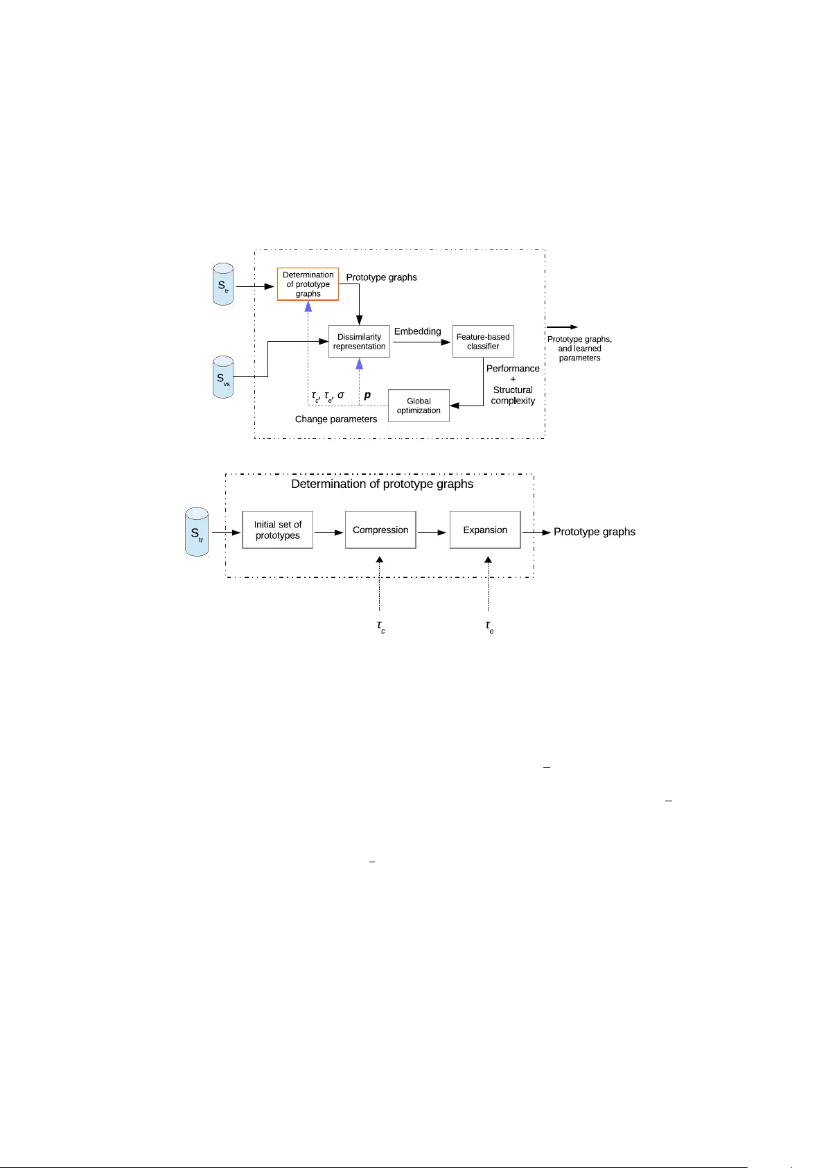
Designing lab eled graph classifiers b y exploiting the R ´ en yi en trop y of the dissimilarit y represen tation Lorenzo Livi ∗ † 1 1 Departmen t of Computer Science, College of Engineering, Mathematics and Physical Sciences, Univ ersity of Exeter, Exeter EX4 4QF, UK Abstract Represen ting patterns as lab eled graphs is b ecoming increasingly common in the broad field of computational in telligence. Accordingly , a wide rep ertoire of pattern recognition to ols, such as clas- sifiers and kno wledge disco very procedures, are now adays av ailable and tested for v arious datasets of lab eled graphs. Ho wev er, the design of effective learning procedures operating in the space of lab eled graphs is still a c hallenging problem, especially from the computational complexit y viewpoint. In this pap er, we presen t a ma jor impro vemen t of a general-purpose classifier for graphs, which is conceiv ed on an interpla y b etw een dissimilarity representation, clustering, information-theoretic tec hniques, and evolutionary optimization algorithms. The improv ement fo cuses on a sp ecific key subroutine devised to compress the input data. W e prov e differen t theorems which are fundamental to the set- ting of the parameters con trolling such a compression op eration. W e demonstrate the effectiveness of the resulting classifier by b enchmarking the developed v ariants on w ell-known datasets of labeled graphs, considering as distinct p erformance indicators the classification accuracy , computing time, and parsimony in terms of structural complexit y of the synthesized classification models. The results sho w state-of-the-art standards in terms of test set accuracy and a considerable sp eed-up for what concerns the computing time. Keywor ds— Graph-based pattern recognition; Classification of lab eled graphs; Dissimilarity repre- sen tation; Information-theoretic data characterization. 1 In tro duction A graph offers a p o werful mo del for represen ting patterns characterized by interacting elements, in b oth static or dynamic scenarios. A lab eled graph (also called attributed graph) is a tuple G = ( V , E , µ, ν ), where V is the finite set of vertices, E ⊆ V × V is the set of edges, µ : V → L V is the v ertex lab eling function, with L V denoting the set of v ertex lab els, and finally ν : E → L E is the edge lab eling function, with L E denoting the set of edge lab els [28]. The top ology of a graph enables the characterization of a pattern in terms of “interacting” elemen ts. Moreo ver, the generality of b oth L V and L E allo ws to co ver a broad range of real-w orld patterns. Applications in volving lab eled graphs for representing data can b e cited in many scientific fields, such as electrical circuits [15], netw orks of dynamical systems [41], bio c hemical netw orks [14, 34], time-v arying lab eled graphs [4], and segmented images [39, 52]. Owing to the rapid diffusion of (c heap) m ulticore computing hardw are, and motiv ated b y the increasing a v ailability of interesting datasets describing complex in teraction-oriented patterns, recent researches on graph-based pattern recognition systems hav e pro duced numerous metho ds [1 – 3, 5, 8, 10 – 12, 16, 18, 27, 32, 33, 35, 36, 38, 53]. F ocusing on the high-level design of classification systems for graphs, it is possible to identify tw o main different approac hes: those that op erate directly in the domain of lab eled graphs and those that deal with the classification problem in a suitable embedding space. Of notable interest are those systems that are based on the so-called explicit gr aph emb e dding algorithms, which transform the input graphs ∗ l.livi@exeter.ac.uk † Corresponding author 1 in to numeric v ectors by means of a mapping or feature extraction technique [28]. Graph embedding algorithms [5, 7, 17, 20, 37, 43, 47, 50], op erate by explicitly developing an embedding space, D . The distance b etw een tw o graphs is hence computed pro cessing their v ector representations in D , usually b y either a geometric or information-theoretic interpretation (e.g., based on div ergences [18]). W e distinguish t wo main categories of graph em b edding algorithms: those that are defined in terms of a core inexact graph matc hing (IGM) pro cedure working directly in the graph domain, G , and those that exploit a matrix representation of the graph to extract characterizing information. The former (e.g., see [5, 7, 47]) can pro cess virtually an y type of lab eled graph, according to the capability of the adopted core matching algorithm. The latter [17, 23, 24, 30, 43, 50] are constrained to pro cess a restricted v ariety of lab eled graphs, in which all the relev an t information can b e effectively enco ded into a matrix representation of a graph, such as (w eighted) adjacency , transition, or Laplacian matrix. The interested reader is referred to [10, 21, 28] and references therein for reviews of recen t graph em b edding tec hniques. The dissimilarity representation offers a v aluable framework for this purp ose, since it p ermits to describ e arbitrarily complex ob jects b y means of their pairwise dissimilarit y v alues (D V) [40]. In the dissimilarit y represen tation, the elements of an input dataset S ⊂ X are characterized by considering v ectors made of their pairwise DVs [40, 51]. The key comp onen t is hence the definition of a nonnegativ e (b ounded) dissimilarity measure d : X × X → R + . A set of prototypes, R , called representation set (RS), is used to dev elop the dissimilarit y matrix (DM), D , whose elements are giv en as D ij = d ( x i , r j ), for every x i ∈ S and r j ∈ R . By means of D , it is p ossible to em b ed the data in S b y developing the so-called dissimilarity space representation: each input sample is represented by the corresponding ro w-vector in D . Recen tly , the Optimized Dissimilarity Space Embedding (ODSE) system has b een prop osed as a general lab eled graph classifier, achieving state-of-the-art results in terms of classification accuracy on w ell-known b enc hmarking datasets [32]. The synthesis of the ODSE classification mo del is p erformed by a no vel information-theoretic in terpretation of the DM in terms of c onveye d information . In practice, the system estimates the informativeness of the input data dissimilarit y represen tation b y calculating the quadratic R´ en yi entrop y (QRE) [42]. Such an entropic characterization has b een used in the compression– expansion scheme as w ell as an important factor of the ODSE ob jective function. Ho wev er, deriving the ODSE classification mo del is computationally demanding. As a consequence, we hav e dev elop ed t wo impro ved versions of the ODSE graph classification system [29], whic h are based on a fast clustering-based compression (CBC) scheme. The parameters of such a clustering algorithm are analytically determined, causing a considerable computational sp eed-up of the mo del synthesis phase, yet maintaining state-of- the-art standards in terms of test set classification accuracy . In this pap er, we elaborate further ov er the same CBC scheme first in tro duced in [29] b y estimating the differen tial α -order R ´ en yi en tropy of the DVs by means of a faster tec hnique that relies on an en tropic Minim um Spanning T ree (MST). Also in this case, w e give a formal pro of p ertaining the setting of the clustering algorithm go verning the compression. W e exp erimen tally demonstrate that the p erformance of ODSE op erating with the MST-based estimator is comparable with the one using the kernel-based estimator. Additionally , w e observ e that with the former the ov erall computing time is in general low er. The remainder of the pap er is organized as follo ws. In T able 1 we report all acronyms used in this pap er. Section 2 provides the necessary theoretical background related to the entrop y estimators used in this work. In Section 3 we give an o verview of the original ODSE graph classification system design [32]. In Section 4 w e present the improv ed ODSE system, whic h is primarily discussed considering the QRE estimator. In Section 4.3, we discuss a relev ant topic related to the (worst-case) efficiency of the dev elop ed CBC pro cedure. Section 5 introduces the principal theoretical contribution of this pap er. W e pro ve a theorem related to the CBC scheme when considering the MST-based estimator. Exp erimen ts and comparisons with other graph classifiers on w ell-known b enc hmarking datasets are presen ted in Section 6. Conclusions and future directions follo w in Section 7. 2 Differen tial R´ en yi entrop y estimators Designing pattern recognition systems by using concepts derived from information theory is now adays w ell-established [42]. A key issue in this context is the estimation of information-theoretic quan tities from a given dataset, such as en tropy and mutual information. F rom the groundbreaking work of Shannon, differen t generalized entrop y form ulations hav e been prop osed. Here we are interested in the 2 T able 1: Acronyms sorted in alphabetic order. Acron ym F ull name BSAS Basic sequential algorithmic sc heme CBC Clustering-based compression DM Dissimilarity matrix DS Dissimilarity space DV Dissimilarity value IGM Inexact graph matc hing MinSOD Minimum sum of distances MMN Min-max network MS Mode Seek MST Minimum spanning tree MST-RE Minim um spanning tree - R´ enyi entropy ODSE Optimized dissimilarity space em b edding QRE Quadratic R´ enyi entrop y RS Represen tation set SOA State-of-the-art SVM Supp ort vector machines TWEC T riple-weigh t edit scheme generalization prop osed by R´ enyi, whic h is called α -order R´ enyi entrop y . Given a con tinuous random v ariable X , distributed according to a probabilit y density function p ( · ), the α -order R ´ enyi entrop y is defined as: H α ( X ) = 1 1 − α log  Z p ( x ) α dx  , α ≥ 0 , α 6 = 1 . (1) In the following tw o subsections, w e pro vide the details of the non-parametric α -order R´ en yi en tropy estimation techniques used here. 2.1 The QRE estimator Recen tly , Pr ´ ıncip e [42] provided a formulation of Eq. 1 in terms of the so-called information p otential of order α , V α ( X ), V α ( X ) = Z p ( x ) α dx ; H α ( X ) = − log  V α ( X ) 1 α − 1  . (2) When α = 2, Eq. 2 simplifies to the so-called quadratic R´ en yi entrop y . Non-parametric kernel-based estimators provide a plug-in solution for the density estimation problem. Typically , a zero-mean Gaussian k ernel G σ ( · ) is adopted, e p ( x ) = 1 n P n i =1 G σ ( x − x i ). The Gaussian kernel G σ ( · ) enables a controllable bias–v ariance trade-off of the estimator dependent on the kernel size σ (and on the data sample size n ). According to Pr ´ ıncip e [42], the QRE of the joint distribution of a d -dimensional random v ector can b e estimated by relying on d different unidimensional kernel estimators combined as follo ws: e V 2 ,σ ( X n ) = 1 n 2 n X i =1 ,j =1 d Y r =1 G σ √ 2  x ( r ) j − x ( r ) i  ! , (3) where e V 2 ,σ ( · ) is the quadratic information p oten tial and G σ √ 2 ( · ) is a conv oluted Gaussian kernel with doubled v ariance, ev aluated at the difference betw een the realizations. Since the input domain is b ounded, the en tropy is maximized when the distribution is uniform, max H 2 ( X ) = d × log(∆), where ∆ is the input data extent [42]. O ( dn 2 ) kernel ev aluations are needed to compute (3), whic h ma y b ecome onerous due to the cost of computing the exp onen tial function. 2.2 The MST-based estimator Let X n b e the data sample of n measurements (p oin ts), with x i ∈ R d , i = 1 , 2 , ..., n , and d ≥ 2, and let G ( X n ) b e the complete (entropic) graph constructed ov er these n measuremen ts. An edge e ij of such a graph connects x i and x j in R d b y means of a straigh t line describ ed by the length | e ij | , which is computed taking the Euclidean distance: | e ij | = d 2 ( x i , x j ) . (4) 3 The α -order R´ enyi en tropy (1) can b e estimated according to a geometric interpretation of a MST of G ( X n ) in R d (shortened as MST-RE). T o this end, let L γ ( X n ) b e the weighte d length of a MST T connecting the n p oin ts, which is defined as L γ ( X n ) = min T ∈T ( G ( X n )) X e ij ∈ T | e ij | γ , (5) where γ ∈ (0 , d ) is a user-defined parameter, and T ( G ( X n )) is the set of all p ossible (entropic) spanning trees of G ( X n ). The R ´ enyi entrop y of order α ∈ (0 , 1), elab orated using the MST length (5), is defined as follows [6, 22]: ˆ H α ( X n ) = d γ  ln  L γ ( X n ) n α  − ln ( β ( L γ , d ))  , (6) where the order α is determined b y calculating: α = d − γ d . (7) The β ( L γ , d ) term is a constant (giv en the data dimensionality) that can b e approximated, for large enough dimensions, d , as: β ( L γ , d ) ' γ 2 ln  d 2 π e  . (8) By mo difying γ we obtain different α -order R ´ en yi en tropies. By definition of G ( X n ), MST-RE (6) is not sensitive to the input dimensionality . Assuming to p erform the estimation on a set of n measurements in R d , the computational complexity in volv ed in computing Eq. 6 is given b y: O  n ( n − 1) 2 e + n ( n − 1) 2 × log  n ( n − 1) 2  + ( n − 1)  . (9) The first term in (9) accoun ts for the generation of G ( X n ), computing the resp ectiv e Euclidean distances for the edge weigh ts. The second term quantifies the cost inv olved in the MST computation using the well-kno wn Krusk al’s algorithm. The last term in (9) concerns the computation of the MST length. 3 The original ODSE graph classifier The ODSE graph classification system [32] is founded on an explicit graph embedding mec hanism that represen ts the input set of graphs S , n = |S | , using a suitable RS R , d = |R| , by initially computing the corresp onding DM, D n × d . The configuration of the em b edding vectors representing the input data in D is deriv ed directly using the rows of D . The adopted IGM dissimilarit y measure is the symmetric v ersion of the procedure called b est matc hing first that uses a three-w eigh t edit scheme (TWEC). Although TWEC pro vides a heuristic solution to the graph edit distance problem, it has sho wn a go od compromise b et ween computational complexit y (quadratic in the graph order) and the num b er of characterizing parameters [5, 28, 32]. TWEC p erforms a greedy assignment of the vertices among the tw o input graphs on the base of the corresp onding labels dissimilarit y; edge op erations are induced accordingly . ODSE synthesizes the classification mo del optimizing the DS representation by means of tw o dedi- cated op erations, called c ompr ession and exp ansion . Both op erations make use of the QRE estimator (Sec. 2.1) to quantify the information conv ey ed by the DM. Another important component of the ODSE graph classification system is the feature-based classifier, whic h op erates directly in D ; its o wn classification mo del is trained during the ODSE synthesis. Such a classifier can b e an y well-kno wn classification system, such as an MMN [48], or a kernelized supp ort v ector mac hine (SVM). T est labeled graphs are classified by ODSE feeding the corresp onding dissimilarity represen tation to the learned feature-based classifier, which assigns proper class lab els to the test patterns. Figs. 1(a) and 1(b) give, respectively , the schematics of the ODSE training and determination of the prototypes. The ODSE classification mo del is defined by the RS, R i , the TWEC parameters, p , and the mo del of the trained feature-based classifier. During the syn thesis stage additional parameters 4 are optimized: the k ernel size σ used by the entrop y estimator and tw o thresholds, τ c , τ e , which are used in the compression and expansion op erations, resp ectiv ely . The ODSE mo del is synthesized by cross-v alidating the learned mo dels on the training set S tr o ver a suitable v alidation set S v s . The global optimization is gov erned by a genetic algorithm, since the recognition p erformance guides, and its analytical definition with resp ect to (w.r.t.) the mo del parameters is not a v ailable in closed form. The genetic algorithm, although it do es not assure conv ergence to wards a global optimum, it is easily and effectiv ely parallelizable, allowing to make use of multicore hardw are/softw are implementations during the training stage. (a) T raining of ODSE. (b) Determination of the prototypes. Figure 1: Schematic descriptions of the main stages in the ODSE training. 3.1 The ODSE ob jectiv e function All parame ters characterizing the ODES mo del are arranged in to co des, c i ∈ C . These include the tw o en tropy thresholds { τ c , τ e } i , the kernel size of the entrop y estimator, { σ } i , the weigh ts of TWEC and an y parameter of the vertex/edge lab el dissimilarity measures, all ranging in [0 , 1]. Since each c i induces a sp ecific RS, R i , the optimization problem that characterizes the ODSE syn thesis consists in deriving the b est-performing RS: ˆ R = arg max c i ∈C f ( S tr , S v s , R i ) . (10) The ob jective function (10) is defined as a linear conv ex combination of tw o ob jectiv es, f ( S tr , S v s , R i ) = η f 1 (Φ R i ( S tr ) , Φ R i ( S v s )) + (1 − η ) f 2 (Φ R i ( S tr )) , (11) where η ∈ [0 , 1] and Φ R i ( · ) shorten the dissimilarity representation of an entire dataset using the compressed-and-expanded RS instance, R i . The function f 1 ( · , · ) ev aluates the recognition rate ac hieved on a v alidation set S v s , while f 2 ( · ) accounts for the quality of the synthesized classification mo del. Sp ecifically , f 2 (Φ R i ( S tr )) = ς Θ + (1 − ς )Υ , (12) 5 where ς ∈ [0 , 1], and Θ denotes the cost related to the num b er d i of prototypes. Accordingly , Θ = 1 − d i − ζ |S tr | , (13) where ζ is the num b er of classes characterizing the classification problem at hand. The second term, namely Υ, captures the informativeness of the DM: Υ = e H 2 ( D n ) . (14) W e consider the entrop y factor (14) in the ODSE ob jectiv e function (11) to increase the spread– disp ersion of the D Vs, which in turn is assumed to magnify the separability of the classes. 3.2 The ODSE compression op eration The compression op eration searc hes for subsets of the initial RS, R , which conv ey similar information w.r.t. S tr ; the initial RS is equal to the whole S tr in the original ODSE. In order to describ e the mec hanism b ehind the ODSE compression op eration, w e need to define when a given subset B ⊆ R of prototypes is compressible. Let D n × d b e the DM corresp onding to S tr and R , with n = |S tr | and d = |R| . Basically , B individuates a subset of k = |B | ≤ d columns of D . Let D [ B ] n × k b e the filter e d DM, i.e., the submatrix considering the prototypes in B only . W e sa y that D [ B ] n × k is compressible if e H 2 ( D k ) ≤ τ c , (15) where 0 ≤ τ c ≤ 1 is the compression threshold, and e H ( · ) estimates the QRE of the underlying join t distribution of D [ B ] n × k . In practice, the v alues of D [ B ] n × k are interpreted as k measurements of a n - dimensional random v ector; D k is the corresp onding notation that we use throughout the paper to denote a sample of k random measuremen ts elaborated from the DM. If the measuremen ts are concen trated around a single n -dimensional supp ort p oin t, the estimated joint entrop y is close to zero. This fact allo ws us to use Eq. 15 as a systematic compression rule, retaining only a single representativ e prototype graph of B . The selection of the subsets B i , i = 1 , 2 , ..., p , for the compressibilit y ev aluation is the first imp ortan t algorithmic issue to b e addressed. In the original ODSE [32], the subset selection has b een p erformed b y means of a randomized algorithm. The computational complexity of this approach is O  d 3 n  , which do es not scale adequately as the input size grows. 3.3 The ODSE expansion op eration The expansion fo cuses on eac h single R j ∈ ← − R , b y analyzing the corresponding columns of the compressed DM, D n × d . By denoting with D n the sample containing the n DVs corresp onding to the j -th column of D , we say that R j is expandable if e H 2 ( D n ) ≤ τ e , (16) where 0 ≤ τ e ≤ 1 is the expansion threshold. Practically , the information pro vided b y the protot yp e is lo w if the n unidimensional measurements are concentrated around a single real-v alued num b er. In such a case, the estimated en tropy would b e low, approaching zero as the underlying distribution b ecomes degenerate. Examples of suc h prototypes are outliers and prototype graphs that are equal in the same measure to all other graphs. Once an expandable R j is individuated through (16), R j is substituted by extracting ζ new graphs elab orated from S tr . Notably , those new graphs are derived by searching for recurren t subgraphs in a suitable subset of the training graphs. Although the idea of trying to extract new features by searching for (recurrent) subgraphs is in ter- esting, it is also very exp ensive in terms of computational complexit y . 4 The impro ved ODSE graph classifier The improv ed ODSE system [29] is designed with the primary goal of a significan t computational sp eed- up. The first v ariant, whic h is presented in Sec. 4.1, considers a simple yet fast RS initialization strategy 6 and a more adv anced compression mechanism. The compression is grounded on a formal result discussed in Sec. 4.1.2. The second v arian t of the ODSE classifier is presented in Sec. 4.2. This v ersion includes a more elab orated initialization of the RS, while it is characterized by the same CBC op eration. The expansion op eration, in b oth cases, has b een greatly simplified. Finally , in Sec. 4.3 we discuss an imp ortan t fact related to the efficiency of the implemen ted CBC. 4.1 ODSE with clustering-based compression op eration 4.1.1 Randomized representation set initialization The initial RS R , that is, the RS used during the syn thesis, is defined by sampling the S tr according to a selection probability , p . The size of the initial RS is th us characterized by a binomial distribution, ing in a verage |S tr | p graphs, with v ariance |S tr | p (1 − p ). Although such a selection criteria is linear in the training set size, it op erates blind ly and may cause an unbalanced selection of the prototypes considering the prior class distributions. Ho wev er, suc h a simple sampling scheme is mostly used when the a v ailable hardw are cannot process the en tire dataset at hand. 4.1.2 Compression by a clustering-based subset selection The entrop y measured b y the QRE estimator (3) is used to determine the compressibilit y of a subset of protot yp es, B . Since the en tropy estimation is directly related to the D Vs b et ween the graphs of B , w e design a subset selection strategy that aggregates the initial prototypes according to their distance in the DS. Such subsets are assured to b e compressible by definition, av oiding thus the computational burden inv olv ed in the entrop y estimation. W e make use of the well-kno wn Basic Sequential Algorithmic Scheme (BSAS) clustering algorithm (see the pseudo-code of Algorithm 1) with the aim of grouping the n -dimensional dissimilarity column- v ectors x j , j = 1 , 2 , ..., d , with (hyper)spheres, using the Euclidean metric d 2 ( · , · ). The main reason b ehind the use of such a simple cluster generation rule is that it is muc h faster than other more sophisticated approac hes [19], and it gives full con trol on the generated cluster geometry through a single real-v alued parameter, θ . Since θ constrains eac h cluster B l to hav e a maximum intra-cluster DV (i.e., a diameter) lo wer or equal to 2 θ , we can deduce analytically the v alue of θ considering the particular instance of the k ernel size σ c and the entrop y threshold τ c used in Eq. 15. Accordingly , the following theorem (see [29] for the proof ) allows us to determine a partition P ( θ ; τ c , σ c ) that con tains clusters that are compressible b y construction. Theorem 1. The c ompr essible p artition P ( θ ; τ c , σ c ) obtaine d on a tr aining set S tr of n gr aphs, is derive d setting: θ ≤ r τ c nσ 2 c ln(2) 2 . (17) Algorithm 1 BSAS clustering algorithm. Input: n input data, a dissimilarit y measure d ( · , · ), cluster radius θ , and maximum num b er of clusters Q Output: P artition P ( θ ) 1: for i = 1 , 2 , ..., n do 2: if P ( θ ) = ∅ then 3: Create a new cluster in P ( θ ) and define x i as the set representativ e 4: else 5: Get the distance v alue D from the closest representativ e mo deling a cluster of the current partition P ( θ ) 6: D = min µ j ∈ P ( θ ) d ( x i , µ j ) 7: if D > θ AND | P ( θ ) | < Q then 8: Add a new cluster in P ( θ ) and define x i as the representative 9: else 10: Add x i in the j -th cluster and up date the representativ e elemen t 11: end if 12: end if 13: end for The optimization of parameters τ c and σ c , together with the pro of of Theorem 1, allows us to search for the b est lev el of training set compression for the problem at hand. Algorithm 2 sho ws the pseudo-co de 7 of the herein describ ed compression op eration. Since the ultimate aim of the compression is to aggregate protot yp es that conv ey similar information w.r.t. S tr , w e represent a cluster using the minimum sum of distances (MinSOD) technique [13]. In fact, the MinSOD allows to select a single representativ e element x k ∈ B k according to the following expression: x k = arg min x j ∈B k X x i ∈B k d 2 ( x j , x i ) . (18) Ev entually , the p protot yp e graphs, B i , i = 1 , 2 , ..., p , corresponding to the p computed MinSOD elemen ts in the DS, p opulate the compressed RS, ← − R = { B 1 , B 2 , ..., B p } . Algorithm 2 Clustering-based compression algorithm. Input: The initial set of prototype graphs R , |R| = d , the DM D n × d , the compression threshold τ c , and the kernel size σ c Output: The compressed set of protot yp e graphs ← − R 1: Configure BSAS setting Q = |R| and θ according to Eq. 17 2: Let X = ( x 1 , x 2 , ..., x d ) be the (ordered) set of dissimilarit y vectors elab orated from the columns of D 3: Execute the BSAS on X . Let P ( θ ; τ c , σ c ) = {B 1 , B 2 , ..., B p } be the obtained compressible partition 4: Compute the MinSOD element b i of each cluster B i , i = 1 , 2 , ..., p , according to Eq. 18. Retriev e from R the prototype graph B i corresponding to eac h dissimilarity vector b i 5: Define ← − R = S p i =1 B i 6: return ← − R The search interv al for the kernel size σ c can b e effectively reduced as follows: 0 ≤ σ c ≤ s 8 ln(2) . (19) A pro of for (19) can b e found in [29]. This bound is imp ortan t, since it allows to narrow the search in terv al for the kernel size σ c , which is theoretically defined in the en tire extended real line. 4.1.3 Expansion based on replacemen t with maxim um dissimilar graphs The genetic algorithm ev olves a population of mo dels o ver the iterations t = 1 , 2 , ..., max. Let R 0 b e defined as sho wn in Sec. 4.1.1, and let N t = S tr \ R t − 1 b e the set of unselected training graphs at iteration t ≥ 1. Finally , let ← − R t b e the compressed RS at iteration t . The herein describ ed expansion op eration makes use of the elements of N t replacing in ← − R t those protot yp es that do not discriminate the classes. The chec k for the expansion of a single prototype graph is still p erformed as describ ed in Sec. 3.3. Notably , if the estimated en tropy from the j -th column vector is lo wer than the expansion threshold, τ e , then l new training graphs are selected from N t for each class, where l ≥ 1 is user-defined. Those ζ × l new graphs are selected suc h that they result maximally dissimilar w.r.t. the j -th prototype under analysis. The new expansion procedure is outlined in [29, Algorithm 2]. Since compression and expansion are ev aluated considering tw o differen t in terpretations of the DM, w e accordingly use t wo different k ernel sizes: σ c and σ e . 4.1.4 Analysis of computational complexit y The computational complexity is dictated by the exec ution of the genetic algorithm, O ( I + E P × F ). I is the cost of the RS initialization, E is the num b er of (maxim um) ev olutions, P is the p opulation size, and finally F is the cost related to a single fitness function ev aluation. In this system v ariant, the initialization is linear in the training set size, O ( I ) = O ( |S tr | ); in a verage we select d 0 = b|S tr | p c protot yp es. The detailed cost related to the fitness function, O ( F ), is articulated as the sum of the follo wing costs: O ( F 1 ) = O ( nd 0 g ); O ( F 2 ) = O ( nQC e ); O ( F 3 ) = O  ← − d n 2 × ( N log( N ) + ζ l )  ; O ( F 4 ) = O  n d  ; O ( F 5 ) = O  v ×  d + k n  ; O ( F 6 ) = O  n 2 d  . (20) 8 The first cost, F 1 , is related to the computation of the initial DM corresp onding to S tr with RS obtained through the initialization of Sec. 4.1.1; g is the computational cost asso ciated with the adopted IGM procedure. F 2 is due to the compression operation which consists in a single BSAS execution, where C = d 0 is the cache size of the MinSOD [13], Q = d 0 , and e = n is the cost of a single Euclidean distance computation. F 3 is the cost c haracterizing the expansion op eration; N is the cardinality of the set N t . This op eration is rep eated at most ← − d = | ← − R | times, with a quadratic entrop y estimation cost in the training set size. F 4 is the cost related to the embedding of the DM, and F 5 is due to the classification of the v alidation set using a k -NN rule based classifier – this cost is up dated according to the sp ecific classifier. F 6 is the cost for the QRE ov er the compressed-and-expanded DM. As it is p ossible to deduce from Eq. 20, the mo del synthesis is now characterized by a quadratic cost in the training set size, n , as well as in the RS size, d , while in the original ODSE it was (pseudo) cubic in b oth n and d . 4.2 ODSE with mo de seeking initialization The ODSE version describ ed here does not include any expansion operation. The RS initialization is no w part of the synthesis, since it dep ends on some of the parameters tuned during the optimization. Compression is still implemented as describ ed in Sec. 4.1.2. The initialization mak es use of the Mode Seek (MS) algorithm [40], which is a w ell-known pro cedure that is able to individuate the mo des of a distribution. F or each class c i , i = 1 , 2 , ..., ζ , and considering a user-defined neighborho od size s ≥ 1, the algorithm pro ceeds as illustrated in [29, Algorithm 3]. The elemen ts of R found in this w ay are the estimated mo des of the class distribution; hence it is a sup ervised algorithm. The cardinalit y of R depends on the choice of s : the larger is s , the smaller R . This approach is very appropriate when elements of the same class are distributed in differen t and heterogeneous clusters: the cluster representativ es are the modes individuated b y the MS algorithm. Moreo ver, the MS algorithm can b e useful to filter out outliers, since they are c haracterized by a lo w neighborho o d density . The pro cedure dep ends on s , which directly influences the outcome of the initialization. Additionally , since the neigh b orho od is defined in the graph domain, MS is also dep endent on the w eights characterizing TWEC (in our case). F or this v ery reason, the initialization is no w p erformed during the ODSE syn thesis. T o limit the complexity of such an initialization, in the exp erimen ts w e systematically assign small v alues to s , constraining the searc h in small neighborho ods. A p ossible side effect of this c hoice is that w e can find an excessiv e num b er of protot yp es/mo des. This effect is how ever atten uated b y the compression algorithm (2). 4.2.1 Analysis of computational complexit y The ov erall computational cost of the synthesis is now b ounded by O ( E P × F ); see (21). The tw o main steps of the fitness function inv olve the execution of the MS algorithm follow ed by the compression algorithm. The F 1 cost refers to the MS algorithm. | c i | is the num ber of training data b elonging to the i -th class. F 2 refers to the computation of the initial DM, constructed using S tr and the d 0 ≤ |S tr | protot yp es deriv ed with MS. F 3 is the cost of the compression operation, with Q = d 0 . F 4 , F 5 , and F 6 are equiv alen t to the ones describ ed in Sec. 4.2.1. The o verall cost is dominated b y the initialization stage (the F 1 cost), which is (pseudo) quadratic in the class size | c i | , and quadratic in the neigh b orho od size, s . O ( F 1 ) = O  n + ζ | c i | ×  | c i | g + | c i | log( | c i | ) + s + s 2  ; O ( F 2 ) = O ( nd 0 g ); O ( F 3 ) = O ( nQC e ); (21) O ( F 4 ) = O  nd  ; O ( F 5 ) = O  v ×  d + k n  ; O ( F 6 ) = O  n 2 d  . 4.3 The efficiency of the ODSE clustering-based compression BSAS (see Algorithm 1) is characterized by a linear computational complexit y . How ev er, due to the sequen tial pro cessing nature, the outcome is sensitive to the data presen tation order. In the following, 9 w e study the effect caused by the ordering of the input o ver the effectiveness of the CBC, b y calculating what we called ODSE c ompr ession efficiency factor. Let s = ( x 1 , x 2 , ..., x n ) b e the sequence of dissimilarity v ectors describing the n protot yp es in the DS, whic h are presen ted in input to Algorithm 1. Let Ω( s ) b e the set of all p erm utations of the sequence s . W e define the optimal compression ratio ρ ∗ ( s ) for the sequence s as: ρ ∗ ( s ) = max s i ∈ Ω( s ) ρ ( s i ) = max s i ∈ Ω( s ) |R| / | ← − R i | , (22) where ← − R i is the compressed RS obtained by analyzing the prototypes arranged according to s i , and R is the uncompressed RS, i.e., the initial RS. Let ˆ ρ ( s ) b e the effectiv e compression ratio, ac hieved by ODSE considering a generic ordering of s . The ratio ξ = lim n →∞ ˆ ρ ( s ) /ρ ∗ ( s ) ∈ [0 , 1] , (23) describ es the asymptotic efficiency of the ODSE compression as the initial RS size gro ws. Theorem 2. The asymptotic worst-c ase ODSE c ompr ession efficiency factor is ξ = 2 / 3 . The pro of can b e found in App endix A. An interpretation of the result of Theorem 2 is that, in the general case, the asymptotic efficiency of the implemented CBC v aries within the [2 / 3 , 1] range of the optim um compression. 5 ODSE with the MST-based R´ en yi en trop y estimator In the follo wing, we contextualize the MST-RE estimation tec hnique in tro duced in Sec. 2.2 as a comp o- nen t of the impro ved ODSE system presented in Sec. 4. Notably , w e provide a theorem for determining the θ parameter of BSAS used in the compression operation (Algorithm 2). In this case, w e generate clusters according to the particular instance of τ c and of the γ parameter, since the k ernel size parameter, σ c , is not presen t in the MST-based estimator. The γ parameter is optimized during the ODSE syn thesis. While γ is defined in (0 , d ), where d is the dimensionality of the samples, w e restrict the searc h interv al to (0 , U ], with U = 3 in the experiments. This tec hnical choice is motiv ated by the fact that γ is used in Eq. 5 as exponent, and an excessively large v alue would easily cause overflow problems of the MST length v ariable floating-p oin t representation. Theorem 3. Considering the instanc es of γ and τ c , the c ompr essible p artition P ( θ ; τ c , γ ) is derive d exe cuting the BSAS algorithm on n = |S tr | tr aining gr aphs by setting: θ ≤ 2 τ c − 1 n τ c 2 β − τ c +1 γ c ( γ ) , where 0 ≤ c ( γ ) ≤ 2 α γ . (24) The pro of of this theorem can b e found in App endix B. Defining θ according to Eq. 24 constrains the BSAS to generate clusters that are compressible by construction. Since τ c and γ are optimized during the synthesis of the classifier, the result of Theorem 3, likewise the one of Theorem 1, allo ws us to ev aluate differen t lev els of training set compression according to the ov erall system p erformance. It go es without saying that computational complexit y discussed in the previous sections is readily up dated b y considering the cost of the MST-based estimator (see Eq. 9). 6 Exp erimen ts In Sec. 6.1 w e introduce the IAM benchmarking datasets. In Sec. 6.2 we present experimental setting. Finally , in Sec. 6.3 we sho w and discuss the results. 6.1 Datasets The experimental ev aluation is performed on the w ell-known IAM graph b enc hmarking databases [44]. The IAM rep ository contains man y different datasets represen ting real-world data collected from v arious fields: from images to biochemical compounds. In particular, we use the L etter LOW (L-L), L etter MED 10 (L-M), L etter HIGH (L-H), AIDS (AIDS), Pr oteins (P), GREC (G), Mutagenicity (M), and finally the Coil-Del (C-D) datasets. The first three are datasets of digitized characters mo deled as lab eled graphs, which are c haracterized by three differen t levels of noise. The AIDS, P , and M datasets represent bio c hemical netw orks, while G and C-D are images of v arious type. F or the sake of brevit y , we rep ort only essential details in T ab. 2, referring the reader to Ref. [44] (and references therein) for a more in- depth discussion ab out the data. Moreov er, since each dataset contains graphs c haracterized by differen t v ertex and edge lab els, we adopted the same vertex and edge dissimilarity measures described in [5, 32]. T able 2: IAM datasets. See [44] for details. DS # (tr, vs, ts) Classes Avg. |V | Avg. |E | L-L (750, 750, 750) 15 4.7 3.1 L-M (750, 750, 750) 15 4.7 3.2 L-H (750, 750, 750) 15 4.7 4.5 AIDS (250, 250, 1500) 2 15.7 16.2 P (200, 200, 200) 6 32.6 62.1 G (286, 286, 528) 22 11.5 12.2 M (1500, 500, 2337) 2 30.3 30.8 C-D (2400, 500, 1000) 100 21.5 54.2 6.2 Exp erimen tal setting The ODSE system version describ ed in Sec. 4.1 is denoted as ODSE2v1, while the v ersion describ ed in Sec. 4.2 as ODSE2v2. These t wo v ersions make use of the QRE estimator; the setting of the clustering algorithm parameter θ used during the compression is hence p erformed according to the result of Theorem 1. By following the same algorithmic scheme, we consider tw o additional ODSE v ariants that differ only in the use of the MST-RE estimator. W e denote those tw o v arian ts as ODSE2v1- MST and ODSE2v2-MST. The setting of θ is hence p erformed according to the pro of of Theorem 3. Ho wev er, the MST-based estimator is conceived for high-dimensional data. As a consequence, in the ODSE2v1-MST system v ersion we still use the QRE estimator in the expansion op eration. W e adopted t wo core classifiers op erating in the DS. The first one is a k -nearest neighbors ( k -NN) rule based classifier equipp ed with the Euclidean distance, testing three v alues of k : 1, 3, and 5. W e also consider a fast MMN, whic h is trained with the AR C algorithm [48]. The four aforemen tioned ODSE v ariants (i.e., ODSE2v1, ODSEv2, ODSEv1-MST, and ODSE2v2-MST) are therefore replicated into additional four v ariants that are straightforw ardly denoted as ODSE2v1-MMN, ODSEv2-MMN, ODSEv1-MST-MMN, and ODSE2v2-MST-MMN, meaning that we just use the neuro-fuzzy MMN on the embedding space, instead of the k -NN. T ab. 3 summarizes all ODSE configurations ev aluated in this pap er. T ests are executed setting the genetic algorithm with a (fixed) p opulation size of 30 individuals, and p erforming a maxim um of 40 evolutions for the syn thesis; a chec k on the fitness v alue is ho wev er p erformed terminating the optimization if the fitness do es not change for 15 ev olutions. This setup has b een c hosen to allow a fair comparison with the previously obtained results [29, 32]. The genetic algorithm p erforms roulette wheel selection, t w o-p oin t crosso ver, and random m utation on the aforemen tioned codes c i , enco ding the real-v alued mo del parameters; in addition, the genetic algorithm implemen ts an elitism strategy which automatically imp orts the fittest individual in to the next p opulation. In all configurations, w e executed the system setting η = 0 . 9 and ς = 0 . 2 in Eq. 11 and 12, resp ectively . Moreo ver, the s parameter affecting the MS algorithm has b een set as follo ws: 10 for the L-L, L-M, and L-H, 20 for AIDS, 2 for P , 8 for G, and finally 100 for either M and C-D. Note that these v alues has b een defined according to the training dataset sizes and considering some preliminary tests. Each dataset has b een pro cessed fiv e times using different random seeds, rep orting hence the av erage test set classification accuracy together with its standard deviation. W e rep ort also the required av erage serial CPU time and the av erage RS size obtained after the synthesis. T ests hav e b een conducted on a regular desktop machine with an Intel Core2 Quad CPU Q6600 at 2.40GHz and 4Gb of RAM; softw are is implemen ted in C++ on a Linux op erating system using the SP ARE library [31]. Finally , the computing time is measured using the clo ck() routine of the standard ctime library . 11 T able 3: Summary of the ODSE configurations ev aluated in the exp erimen ts. The “Init” column refers to the RS initialization scheme, “Compression / Est.” refers to the compression algorithm and adopted en tropy estimator, “Expansion / Est.” the same but for the expansion algorithm, and “Ob j. F unc. (14)” refers to the entrop y estimator adopted in Eq. 14. Finally , “FB Class.” sp ecifies the feature-based classifier op erating in the DS. Acron ym Init Compression / Est. Expansion / Est. Ob j. F unc. (14) FB Class. ODSE2v1 Sec. 4.1.1 Sec. 4.1.2 / QRE Sec. 4.1.3 / QRE QRE k -NN ODSE2v2 Sec. 4.2 Sec. 4.1.2 / QRE – QRE k -NN ODSE2v1-MST Sec. 4.1.1 Sec. 4.1.2 / MST-RE Sec. 4.1.3 / QRE MST-RE k -NN ODSE2v2-MST Sec. 4.2 Sec. 4.1.2 / MST-RE – MST-RE k -NN ODSE2v1-MMN Sec. 4.1.1 Sec. 4.1.2 / QRE Sec. 4.1.3 / QRE QRE MMN ODSE2v2-MMN Sec. 4.2 Sec. 4.1.2 / QRE – QRE MMN ODSE2v1-MST-MMN Sec. 4.1.1 Sec. 4.1.2 / MST-RE Sec. 4.1.3 / QRE MST-RE MMN ODSE2v2-MST-MMN Sec. 4.2 Sec. 4.1.2 / MST-RE – MST-RE MMN 6.3 Results and discussion All test set classification accuracy results hav e b een collected in T ab. 4. These include the results of three baseline reference systems and several state-of-the-art (SOA) classification systems based on graph em b edding techniques. The table is divided in appropriate macro blo cks to simplify the comparison of the results. The three reference systems are denoted as RPS+TWEC+ k -NN, k -NN+TWEC, and RPS+TWEC+MMN. The first one p erforms a (class-indep endent) randomized selection of the training graphs to develop the dissimilarit y represen tation of the input data. This system adopts the same TWEC used in ODSE and performs the classification in the DS by means of a k -NN classifier equipp ed with the Euclidean distance. The second one differs from the first system by using instead the MMN. Finally , the third reference system op erates directly in G by means of a k -NN rule based classifier equipp ed with TWEC. In all cases, to obtain a fair comparison with ODSE, the configuration of the dissimilarity measures for the v ertex/edge lab els is consistent with the one adopted for ODSE. Additionally , k = 1 , 3, and 5 is used in the k -NN rule, p erforming the TWEC parameters optimization (i.e., the w eighting parameters in [0 , 1]) by means of the same aforementioned genetic algorithm implementation. Therefore, also in this case the test set results m ust b e intended as the av erage of five differen t runs (how ever w e omit standard deviations for the sake of brevit y). T ab. 4 presen ts the obtained test set classification accuracy results, while T ab. 5 gives the cor- resp onding standard deviations. W e pro vide t wo types of statistical ev aluation of suc h results. First, w e p erform pairwise comparisons by means of t -test; we adopt the usual 5% as significance threshold. Notably , we c hec k if any of the impro ved ODSE v ariants significan tly outp erforms, for eac h dataset, b oth the reference systems and original ODSE. Best results satisfying such a condition are rep orted in b old in T ab. 4. In addition to the pairwise comparisons, we calculate also a global ranking of all classifiers b y means of the F riedman te st. Missing v alues are replaced b y the dataset-sp ecific av erages. First of all, w e note that results obtained with the baseline reference systems are alw ays w orse than those obtained with ODSE. T est set classification accuracy p ercen tages obtained b y ODSE2v1-MST and ODSE2v2-MST are comparable with those of ODSE2v1 and ODSE2v2, although w e note a slightly general improv emen t for the first tw o v ariants. Results are also more stable v arying the neighborho o d size parameter, k , of the k -NN rule. It is w orth noting that, for difficult datasets as P and C-D, increasing the neighborho od size in the k -NN rule affects significantly the test set p erformance (i.e., results degrade considerably). T est set classification accuracy results obtained by means of the MMN op erating in the DS are in general (slightly) inferior w.r.t. the ones obtained with the k -NN rule – setting k = 1. This result is not to o unusual since the k -NN rule is a v aluable classifier, esp ecially in absence of noisy data. Since ODSE operates by searc hing for the b est-performing DS for the data at hand, we may deduce that the em b edding vectors are sufficiently w ell-organized w.r.t. the classes. T est set results on the first four datasets (i.e., L-L, L-M, L-H, and AIDS) denote an imp ortan t impro vemen t o ver a large part of the SOA systems. On the other hand, results ov er the P , G, and M datasets are comparable w.r.t. those of the SOA systems. F or all ODSE configurations, we observ e non convincing results on the C-D dataset; in this case results are comparable only with those of the reference systems (first blo c k of T ab. 4). How ev er, a rational reason explaining this fact is not emerged from the tests yet, requiring th us more future inv estigations. The global picture provided b y the column denoted as “Rank” sho ws that 12 the ODSE classifiers rank in general v ery well w.r.t. the SOA systems. Standard deviations (T ab. 5) are reasonably small, denoting a reliable classifier regardless the particular ODSE v arian t. W e demonstrated that the asymptotic computational complexity of ODSE2 is quadratic, while the original ODSE was characterized by a cubic computational complexity . Here, in order to complement this result with exp erimen tal evidence, w e discuss also the effective computing time. The calculated serial CPU time, for each dataset, is shown in T ab. 6, which includes b oth ODSE synthesis and test set ev aluation. The ODSE v ariants based on the MST entrop y estimator are faster, with the only exception for the P and C-D datasets. This fact is magnified on the first four datasets, in whic h the sp eed-up factor w.r.t. the original ODSE increases considerably . The sp eed-up factors obtained for the first three datasets are one order of magnitude higher than the ones obtained in the other datasets. In order to pro vide an explanation for suc h differences, we need to tak e a closer lo ok at the dataset details shown in T ab. 2, computational complexit y in Eqs. 20 and 21, and the computational complexity of the original ODSE [32]. It is possible to notice that the first three datasets con tain smaller (in av erage) lab eled graphs. Therefore, this p oints us to lo ok for the related terms in the computational complexit y formulae. The g term (the cost of the graph matc hing algorithm) is directly affected b y the size of the graphs and app ears in F 1 Eq. 20 and F 1 , F 2 in Eq. 21. The same g term appears also in F 1 of Eq. 24 in [32]. In the original ODSE version [32], the dissimilarity matrix is constructed using an initial set of prototypes equal to the training set (then it is compressed and expanded). In the new version presented here, we instead use a reduced set with d 0 elemen ts. In the first v ariant that w e presen ted, d 0 graphs are selected randomly from the training set based on a selection probabilit y . In the second v arian t, instead, we use the MS algorithm, whic h finds a m uch low er n umber of representativ es (although, as said in the experimental setting section, w e use a conserv ative setting for MS). This fact provides a first rational justification for explaining the aforemen tioned difference s. In fact, graph matching algorithms are exp ensiv e from the computational viewp oin t (the adopted algorithm is quadratic in the num ber of vertices). In addition, compression and expansion op erations are now m uch faster (from cubic to quadratic in time). As sho wn in T ab. 8, the new ODSE versions compute a smaller RS; a direct consequence of the improv ed compression op eration. This is another imp ortan t factor contributing to the ov erall sp eed-up, since smaller RSs imply less graph matc hing computations during the v alidation and test stages (we remind that ODSE is trained by cross- v alidation). Clearly , there are also other factors, such as the conv ergence of the optimization algorithm, whic h might b e affected by the sp ecific dataset at hand. As exp ected, the sp eed-up factors obtained by using the MMN as classifier are in general higher than those obtained with kNN. In fact, the MMN syn thesizes a classification mo del ov er the training data embedded in to a DS. This significantly reduces the computing time necessary for the ev aluation of the test set (and also of the v alidation stage p erformed during the syn thesis of the mo del). This is demonstrated b y the results in T ab. 7, where we rep ort the CPU time for the test set ev aluation only . This fact might assume more imp ortance in particular applications, esp ecially in those where the syn thesis of the classifier can b e effectively p erformed only once in off-line mo de and the classification mo del is employ ed to pro cess high-rate data streams in real-time [49]. Let us fo cus no w on the structural complexit y of the syn thesized classification mo dels. The cardinalit y of the best-p erforming RSs are sho wn in T ab. 6. It is p ossible to note that the cardinalit y are slightly bigger for those v ariants operating with MST-RE (esp ecially in the first three datasets, i.e., L-L, L- M, and L-H). F rom this fact we deduce that, when configuring the CBC pro cedure with the MST-RE estimator, the ODSE classifier, in order to obtain goo d results in terms of test set accuracy , requires a more complex mo del w.r.t. the v ariants in volving the QRE estimator. This b eha vior is how ev er magnified by the setting of the ob jectiv e function parameter η adopted in our tests, which biases the ODSE system tow ards the recognition rate p erformance. Notably , v ariants op erating with the MMN dev elop considerable less costly classification mo dels (see T ab. 8 and 9 for the details). This particular asp ect b ecomes v ery imp ortan t in resource-constrained scenarios and/or when the input datasets are v ery big. The considerable reductions of the RS size here ac hieved strengthen the fact that the entrop y estimation op erates adequately in the dissimilarit y representation con text. 7 Conclusions and future directions In this pap er, we ha ve presented differen t v ariants of the improv ed ODSE graph classification system. All the discussed v ariants are based on the c haracterization of the informativ eness of the DM through the 13 T able 4: T est set classification accuracy results – gra yed lines denote nov el results introduced in this pap er. The “-” sign means that the result is not a v ailable to our knowledge. Classifier Dataset Rank L-L L-M L-H AIDS P G M C-D Reference systems RPS+TWEC+ k -NN, k = 1 98.4 96.0 95.0 98.5 45.5 95.0 69.0 81.0 15 k -NN+TWEC, k = 1 96.8 66.3 36.3 73.9 52.1 95.0 57.7 61.2 38 RPS+TWEC+ k -NN, k = 3 98.6 97.2 94.7 98.2 40.5 92.0 68.7 63.2 23 k -NN+TWEC, k = 3 97.5 57.4 39.1 71.4 48.5 91.8 56.1 33.7 39 RPS+TWEC+ k -NN, k = 5 98.3 97.1 95.0 97.6 35.4 84.8 68.5 59.7 32 k -NN+TWEC, k = 5 97.6 60.4 42.2 76.7 43.0 88.5 56.9 27.8 40 RPS+TWEC+MMN 98.0 96.0 93.6 97.4 49.5 95.0 66.0 68.4 28 SO A systems GMM+soft all+SVM [20] 99.7 93.0 87.8 - - 99.0 - 98.1 12 F uzzy k -means+soft all+SVM [20] 99.8 98.8 85.0 - - 98.1 - 97.3 9 sk+SVM [45] 99.7 85.9 79.1 97.4 - 94.4 55.4 - 30 le+SVM [45] 99.3 95.9 92.5 98.3 - 96.8 74.3 - 7 PCA+SVM [46] 92.7 81.1 73.3 98.2 - 92.9 75.9 93.6 26 MDA+SVM [46] 89.8 68.5 60.5 95.4 - 91.8 62.4 88.2 37 svm+SVM [9] 99.2 94.7 92.8 98.1 71.5 92.2 68.3 - 17 svm+kPCA [9] 99.2 94.7 90.3 98.1 67.5 91.6 71.2 - 14 lgq [26] 81.5 - - - - 86.2 - - 35 bay es 1 [25] 80.4 - - - - 80.3 - - 36 bay es 2 [25] 81.3 - - - - 89.9 - - 34 FMGE+ k -NN [37] 97.1 75.7 66.5 - - 97.5 69.1 - 31 FMGE+SVM [37] 98.2 83.1 70.0 - - 99.4 76.5 - 21 d-sps-SVM [7] 99.5 95.4 93.4 98.2 73.0 92.5 71.5 - 8 GRALGv1 [5] 98.2 75.6 69.6 99.7 - 97.7 73.0 94.0 10 GRALGv2 [5] 97.6 89.6 82.6 99.7 64.6 97.6 73.0 97.8 6 Original ODSE ODSE, k = 1 [32] 98.6 96.8 96.2 99.6 61.0 96.2 73.4 - 1 Improv ed ODSE with QRE ODSE2v1, k = 1 [29] 99.0 97.0 96.1 99.1 61.2 98.1 68.2 78.1 4 ODSE2v2, k = 1 [29] 98.7 97.1 95.4 99.5 51.9 95.4 68.1 77.2 5 ODSE2v1, k = 3 [29] 99.0 97.2 96.1 99.3 41.4 90.2 68.7 64.3 13 ODSE2v2, k = 3 [29] 98.8 97.4 95.1 99.4 31.4 38.0 69.4 59.0 24 ODSE2v1, k = 5 [29] 99.1 96.8 95.2 99.0 38.9 85.4 69.0 58.6 27 ODSE2v2, k = 5 [29] 98.7 97.0 95.6 99.4 31.3 82.5 70.0 54.0 25 ODSE2v1-MMN 98.3 95.2 94.0 99.3 53.1 94.5 67.9 62.8 22 ODSE2v2-MMN 97.8 95.6 93.6 99.6 48.7 94.8 68.2 59.2 29 Impro ved ODSE with MST-RE ODSE2v1-MST, k = 1 98.6 96.8 98.9 99.3 61.3 95.6 70.0 81.0 3 ODSE2v2-MST, k = 1 98.4 97.1 96.0 99.7 51.0 94.1 71.6 82.0 2 ODSE2v1-MST, k = 3 98.7 97.0 96.8 99.5 43.0 92.3 68.6 64.8 11 ODSE2v2-MST, k = 3 98.8 96.9 96.0 99.7 35.0 91.0 69.4 60.0 16 ODSE2v1-MST, k = 5 99.0 96.8 95.6 99.6 41.4 85.0 68.6 60.0 18 ODSE2v2-MST, k = 5 98.8 97.0 95.5 99.7 32.9 83.3 70.0 54.0 19 ODSE2v1-MST-MMN 97.9 95.4 93.6 99.3 49.9 95.0 68.3 62.6 20 ODSE2v2-MST-MMN 97.9 95.1 91.8 99.2 48.5 94.8 67.1 59.0 33 T able 5: Standard deviations of ODSE results sho wn in T ab. 4. Classifier Dataset L-L L-M L-H AIDS P G M C-D ODSE [32] 0.0256 1.2346 0.2423 0.0000 0.7356 0.4136 0.6586 - ODSE2v1, k = 1 [29] 0.0769 0.2309 0.1539 0.0000 2.6242 1.3350 0.5187 4.3863 ODSE2v2, k = 1 [29] 0.0769 0.0769 0.4000 0.0000 0.2915 0.8021 0.5622 2.2654 ODSE2v1, k = 3 [29] 0.0769 0.2309 0.2666 0.0000 1.0513 1.2236 0.0856 0.0577 ODSE2v2, k = 3 [29] 0.0769 0.4618 5.0800 0.1924 1.1666 3.1540 0.0356 1.2361 ODSE2v1, k = 5 [29] 0.5047 0.0769 0.9365 0.1924 0.5050 2.5585 0.3803 1.3279 ODSE2v2, k = 5 [29] 0.1333 0.2309 0.0769 0.0000 2.7815 4.5220 1.2666 0.0026 ODSE2v1-MMN 0.1520 0.3320 0.3932 0.1861 1.7740 0.7315 1.1300 1.0001 ODSE2v2-MMN 0.2022 0.2022 0.7682 0.0000 2.7290 1.3584 1.4080 0.3896 ODSE2v1-MST, k = 1 0.0730 0.0730 0.1115 0.2772 1.5500 0.1055 1.0786 0.4163 ODSE2v2-MST, k = 1 0.0596 0.2231 0.0730 0.0000 1.1660 0.2943 0.9534 0.2146 ODSE2v1-MST, k = 3 0.1192 0.1520 0.0942 0.6982 1.0940 0.0000 0.5926 1.7088 ODSE2v2-MST, k = 3 0.1460 0.2022 0.0730 0.0000 0.0000 0.1112 0.2365 0.5655 ODSE2v1-MST, k = 5 0.1115 0.0942 0.2190 0.0596 0.4748 0.0000 0.0547 1.2356 ODSE2v2-MST, k = 5 0.0730 0.0596 0.9933 0.0000 0.0000 0.1112 1.0023 0.9563 ODSE2v1-MST-MMN 0.1115 0.4216 0.7624 0.3217 2.5735 0.3067 0.7926 0.9899 ODSE2v2-MST-MMN 0.0596 0.7636 0.7477 0.0000 2.7290 0.5828 0.8911 1.2020 14 T able 6: Average serial CPU time in minutes (and sp eed-up factor w.r.t. the original ODSE system) considering ODSE model syn thesis and test set ev aluation. In the k -NN case, we rep ort the results with k = 1 only . Classifier Dataset L-L L-M L-H AIDS P G M C-D ODSE [32] 63274 52285 28938 394 8460 601 43060 - ODSE2v1 [29] 284 (222) 329 (158) 328 (88) 38 (10) 3187 (3) 210 (3) 3494 (12) 2724 ODSE2v2 [29] 126 (502) 268 (195) 183 (158) 110 (3) 1683 (5) 96 (6) 10326 (4) 8444 ODSE2v1-MMN 129 (490) 284 (184) 263 (110) 17 (23) 3638 (2) 170 (4) 8837 (5) 5320 ODSE2v2-MMN 195 (324) 422 (124) 183 (158) 86 (5) 1444 (6) 77 (8) 28511 (2) 20301 ODSE2v1-MST 213 (297) 231 (226) 225 (129) 18 (22) 3860 (2) 168 (4) 2563 (17) 3261 ODSE2v2-MST 145 (463) 160 (327) 107 (270) 93 (4) 2075 (4) 74 (8) 7675 (6) 10092 ODSE2v1-MST-MMN 201 (315) 249 (210) 205 (141) 15 (26) 3450 (2) 155 (4) 5496 (8) 7135 ODSE2v2-MST-MMN 117 (541) 176 (292) 118 (245) 83 (5) 1380 (6) 75 (8) 28007 (2) 16599 T able 7: Average serial CPU time in seconds for test set ev aluation only . F or simplicity , we rep ort the results of only one system v ariant op erating in the DS with the k -NN classifier and only one with the MMN. Class. Sys. Datasets L-L L-M L-H AIDS P G M C-D ODSE2v1-MST, k = 1 0.740 0.740 0.740 0.130 0.020 0.060 9.020 9.700 ODSE2v1-MST-MMN 0.105 0.105 0.105 0.005 0.014 0.045 6.600 5.250 T able 8: Av erage cardinality of the b est-performing RS. In the k -NN case, w e rep ort the results with k = 1 only since results with k = 3 and k = 5 are similar. Classifier Dataset L-L L-M L-H AIDS P G M C-D ODSE [32] 435 750 750 250 200 283 1500 - ODSE2v1 [29] 146 449 449 8 197 283 760 615 ODSE2v2 [29] 183 431 338 7 82 126 801 770 ODSE2v1-MM 136 192 144 6 190 163 563 555 ODSE2v2-MM 197 546 80 2 93 115 815 740 ODSE2v1-MST 597 595 597 6 198 283 687 618 ODSE2v2-MST 551 574 447 61 122 129 813 775 ODSE2v1-MST-MMN 600 606 500 5 190 184 424 549 ODSE2v2-MST-MMN 550 580 411 61 93 115 456 733 T able 9: Average num ber of hyperb o xes generated by the MMN. The num b er of hyperb o xes can b e used also as a complexity indicator of the mo del synthesized by the MMN on the DS. Such v alues should b e taken in to account considering also the dataset c haracteristics of T ab. 2 and the computed av erage represen tation set sizes in T ab. 8. Classifier Dataset L-L L-M L-H AIDS P G M C-D ODSE2v1-MMN 15 39 34 5 43 27 164 357 ODSE2v2-MMN 15 28 41 4 48 28 159 368 ODSE2v1-MST-MMN 15 27 38 3 48 28 168 348 ODSE2v2-MST-MMN 15 27 34 4 43 27 175 365 15 estimation of the α -order R´ en yi entrop y . The first adopted estimator computes the QRE by means of a k ernel-based density estimator, while the second one uses the length of an en tropic MST. The impro ved ODSE system has b een designed b y pro viding differen t strategies for the initialization, compression, as w ell as for the expansion operation of the RS. In particular, w e conceiv ed a fast CBC scheme, which allo wed us to directly control the compression level of the data through the explicit setting of the cluster radius parameter. W e provided formal proofs for the t wo estimation tec hniques. These pro ofs enabled us to determine the v alue of the cluster radius analytically , according to the ODSE model optimization pro cedure. W e ha ve studied also the asymptotic w orst-case efficiency of the CBC scheme implemented b y means of a sequen tial cluster generation rule (BSAS). Exp erimen tal ev aluations and comparisons with several state-of-the-art systems ha ve been p erformed on well-kno wn b enc hmarking datasets of lab eled graphs (IAM database). W e used t wo different feature- based classifiers op erating in the DS: the k -NN classifier equipp ed with the Euclidean distance and a neurofuzzy MMN trained with the AR C algorithm. Overall, the v arian ts adopting the MST-based estimator resulted to be faster but less parsimonious for what concerns the syn thesized ODSE mo del (i.e., the cardinality of the b est-performing RS was larger). The use of the k -NN rule (with k = 1) yielded sligh tly b etter test set accuracy results w.r.t. the MMN, while ho wev er in the latter case w e ha ve observed imp ortant differences in term of (serial) CPU computing time, esp ecially on the test set pro cessing stage. The test set classification accuracy results confirmed the effectiv eness of the ODSE classifier w.r.t. state-of-the-art standards. Moreo ver, the significative CPU time impro vemen ts w.r.t. the original ODSE version, and the highly parallelizable global optimization scheme based on a genetic algorithm, bring the ODSE graph classifier one step closer tow ards the applicabilit y to bigger labeled graphs and larger datasets. The v ector representation of the input graphs hav e b een obtained directly using the rows of the dissimilarit y matrix. Suc h a choice, while it is known to b e effective, has b een mainly dictated by the computing time requirements of the system. It is w orth analyzing the p erformance of ODSE also when the embedding space is obtained by a (non)linear embedding of the (corrected) pairwise dissimilarity v alues [54]. F uture exp erimen ts include testing other core IGM pro cedures, different α -order R ´ en yi en tropy estimators, and additional feature-based classifiers. A Pro of of Theorem 2 Pr o of. W e fo cus on the worst-case scenario for ξ , giving th us a low er b ound for the efficiency (23). Let s [ i ] = x i denote the i -th element of the sequence s , i.e., the i -th dissimilarity v ector corresp onding to the prototype graph R i ∈ R . Let s ∗ b e the b est ordering for s , i.e., s ∗ = arg max s i ∈ Ω( s ) ρ ( s i ) . (25) Let us assume the case in which the Euclidean distance among any pair of v ectors in s is giv en by d 2 ( s [ i ] , s [ j ]) = | i − j | θ , 1 ≤ i, j ≤ n, (26) where θ is the adopted cluster radius during the ODSE compression. It is easy to understand that this is the worst-case scenario for the compression purp ose in the sequen tial clustering setting. In fact, eac h v ector x i in the sequence s has a distance with its predecessor/successor equal to the maximum cluster radius θ . As a consequence, there is still a p ossibility to compress the v ectors, but it is how ev er strictly dep enden t on the sp ecific ordering of s . First of all, it is imp ortan t to note that, due to the distances assumed in (26), only three elements of s can b e con tained in to a single cluster. In fact, an y three consecutive elements of the sequence s w ould form a cluster with a diameter equal to 2 θ . Therefore, considering the sequential rule shown in Algorithm 1, and setting Q = n , the b est possible ordering s ∗ is the one that preserv es a distance equal to θ for an y t wo adjacent elemen ts of s , achieving a compression ratio of: ρ ∗ ( s ) = n/ d n/ 3 e . (27) The w orst p ossible ordering, instead, yields n/ d n/ 2 e , whic h can b e ac hieved (for instance assuming n o dd) when considering the follo wing ordering s i w.r.t. the optimal s ∗ : s i [ j ] = s ∗ [(2 j mo d n ) + 1] , j = 1 , 2 , ..., n. (28) 16 In this case, Algorithm 1 would generate exactly d n/ 2 e (29) clusters, corresp onding to the first d n/ 2 e elements of the sequence s i , since every pair of consecutive elemen ts in s i is at a distance of exactly 2 θ . Therefore, d n/ 2 e is the maximum num b er of clusters that can b e generated b y considering the distances assumed in (26). Combining Eq. 27 and 29, we obtain for a given s , n/ d n/ 2 e ≤ ˆ ρ ( s ) ≤ ρ ∗ ( s ) = n/ d n/ 3 e , (30) whic h allows us to claim that the w orst-case efficiency of the ODSE compression v aries according to the follo wing ratio: ˆ ρ ( s ) /ρ ∗ ( s ) = n d n/ 2 e × d n/ 3 e n = d n/ 3 e d n/ 2 e . (31) T aking the limit for n → ∞ in Eq. 31 gives us the claim. B Pro of of Theorem 3 Pr o of. Let us fo cus the analysis on a single cluster B ∈ P ( θ ; τ c , γ ), containing k = |B | prototypes within a training set of n graphs. Let us remind that the cluster radius and diameter are, respectively , θ and 2 θ in the spherical cluster case. Therefore, we can obtain an upp er b ound for the MST length factor (5), c onsidering that (all) the corresp onding MST, T , of the complete graph generated from the k measuremen ts has k − 1 edges with weigh ts equal to 2 θ . Sp ecifically , L γ ( θ ) = X e ij ∈ T | e ij | γ = ( k − 1) × (2 θ ) γ . (32) In the follo wing, w e ev aluate β ( L γ ( θ ) , n ) exactly as defined in Eq. 8, considering n dimensions – note that β ( L γ ( θ ) , n ) is shortened as β . Eq. 32 allows us to deriv e the following upp er b ound for the MST-based entrop y estimator (6): ˆ H α ( D k ) = n γ  ln  L γ ( D k ) k α  − ln ( β ( L γ , n ))  ≤ n γ  ln  L γ ( θ ) k α  − ln( β )  = n γ  ln  ( k − 1) × (2 θ ) γ k α  − ln( β )  = n γ [ln( k − 1) + γ ln(2 θ ) − ln( k α ) − ln( β )] . (33) Ho wev er, the entrop y estimator shown in Eq. 6 do es not yield normalized v alues (e.g., in [0 , 1]). W e can normalize the estimations by considering the follo wing factor: ι = n γ  ln( k − 1) + γ ln(∆ √ n ) − ln( k α ) − ln( β )  . (34) The quan tity ∆ √ n is the maxim um distance in an Euclidean ∆-hypercub e of n -dimensions; ∆ is the input data extent, whic h is 2 in our case. Eq. 34 is a maximizer of Eq. 6 since the logarithm is a monotonically increasing function and the other relev ant factors in the expression remain constant c hanging the input distribution. Instead, the MST length ac hieves its maxim um v alue only in the specific case when all k p oin ts are at a distance equal to 2 √ n . Therefore, by normalizing Eq. 33 using (34), we obtain: ln( k − 1) + γ ln(2 θ ) − ln( k α ) − ln( β ) ln( k − 1) + γ ln(2 √ n ) − ln( k α ) − ln( β ) ∈ [0 , 1] . (35) Rewriting the expression in terms of the ODSE compression rule (15), we hav e: ˆ H α ( D k ) ι ≤ ln( k − 1) + γ ln(2 θ ) − ln( k α ) − ln( β ) ln( k − 1) + γ ln(2 √ n ) − ln( k α ) − ln( β ) ≤ τ c . (36) 17 Solving for θ , the righ t-hand side of (36) can b e manipulated as follo ws: γ ln(2 θ ) ≤ τ c  ln( k − 1) + γ ln(2 √ n ) − ln( k α ) − ln( β )  − ln( k − 1) + ln( k α ) + ln( β ); ln(2 θ ) ≤ τ c γ  ln( k − 1) + γ ln(2 √ n ) − ln( k α ) − ln( β )  + 1 γ [ − ln( k − 1) + ln( k α ) + ln( β )] ; θ ≤ 1 2 exp  τ c γ  ln( k − 1) + γ ln(2 √ n ) − ln( k α ) − ln( β )   × exp  1 γ [ − ln( k − 1) + ln( k α ) + ln( β )]  ; θ ≤ 1 2  exp  ln( k − 1) + γ ln(2 √ n ) − ln( k α ) − ln( β )  τ c γ × [exp ( − ln( k − 1) + ln( k α ) + ln( β ))] 1 γ ; θ ≤ 1 2 h ( k − 1)2 γ n γ 2 k − α β − 1 i τ c γ  ( k − 1) − 1 k α β  1 γ ; θ ≤ 1 2 ( k − 1) τ c γ 2 τ c n τ c 2 k − ατ c γ β − τ c γ ( k − 1) − 1 γ k α γ β 1 γ ; θ ≤ ( k − 1) τ c − 1 γ 2 τ c − 1 n τ c 2 k α ( − τ c +1) γ β − τ c +1 γ . (37) Considering that τ c − 1 ≤ 0 and ( − τ c + 1) ∈ [0 , 1] hold for an y τ c ∈ [0 , 1], w e rewrite Eq. 37 accordingly as follows: θ ≤ 2 τ c − 1 n τ c 2 β − τ c +1 γ k α ( − τ c +1) γ ( k − 1) − τ c +1 γ ; (38) θ ≤ 2 τ c − 1 n τ c 2 β − τ c +1 γ  k α ( k − 1)  − τ c +1 γ . (39) The right-hand side of Eq. 39 can b e further simplified in: θ ≤ 2 τ c − 1 n τ c 2 β − τ c +1 γ c ( γ ) , (40) where the c ( γ ) function has the follo wing b ounds: 0 ≤ c ( γ ) ≤  k α k − 1  − τ c +1 γ . (41) In fact, pro vided that α ∈ (0 , 1) and k ∈ N hold, with k ≥ 2 (there is no need to compress singleton clusters), we hav e:    k α ( − τ c +1) γ ( k − 1) τ c − 1 γ = 0 if k → ∞ , k α ( − τ c +1) γ ( k − 1) τ c − 1 γ =  k α k − 1  − τ c +1 γ otherwise . (42) Note that c ( γ ) dep ends also on α , which, ho wev er, in turn dep ends on γ (7); as a conv ention we express c ( γ ) as a function of the γ parameter only . Eq. 42 ev aluates to 2 α γ when k = 2 and τ c = 0, pro viding hence the upper bound for c ( · ). References [1] L. Bai and E. R. Hanco c k. Graph Kernels from the Jensen-Shannon Divergence. Journal of Mathematic al Imaging and Vision , 47(1-2):60–69, 2013. doi: 10.1007/s10851- 012- 0383- 6. [2] L. Bai, L. Rossi, A. T orsello, and E. R. Hanco ck. A quan tum Jensen–Shannon graph kernel for unattributed graphs. Pattern R e c ognition , 48(2):344–355, 2015. ISSN 0031-3203. doi: 10.1016/j.patcog.2014.03.028. 18 [3] E. Bengo etxea, P . Larra ˜ naga, I. Blo c h, A. Perchan t, and C. Bo eres. Inexact graph matching b y means of estimation of distribution algorithms. Pattern R e c o gnition , 35(12):2867–2880, 2002. ISSN 0031-3203. doi: 10.1016/S0031- 3203(01) 00232- 1. [4] F. M. Bianc hi, L. Livi, and A. Rizzi. Matching of time-v arying labeled graphs. In Pro c e e dings of the IEEE International Joint Confer enc e on Neur al Networks , pages 1660–1667, Aug 2013. ISBN 978-1-4673-6129-3. doi: 10.1109/IJCNN. 2013.6706939. [5] F. M. Bianchi, L. Livi, A. Rizzi, and A. Sadeghian. A Granular Computing approach to the design of optimized graph classification systems. Soft Computing , 18(2):393–412, 2014. ISSN 1432-7643. doi: 10.1007/s00500- 013- 1065- z. [6] B. Bonev, F. Escolano, and M. Cazorla. F eature selection, mutual information, and the classification of high- dimensional patterns. Pattern Analysis and Applic ations , 11(3-4):309–319, 2008. ISSN 1433-7541. doi: 10.1007/ s10044- 008- 0107- 0. [7] E. Z. Borzeshi, M. Piccardi, K. Riesen, and H. Bunk e. Discriminativ e protot yp e selection methods for graph em b edding. Pattern R e c ognition , 46(6):1648–1657, 2013. ISSN 0031-3203. doi: 10.1016/j.patcog.2012.11.020. [8] S. R. Bul` o and M. Pelillo. A game-theoretic approach to hypergraph clustering. IEEE T r ansactions on Pattern Analysis and Machine Intel ligenc e , 35:1312–1327, Jun. 2013. ISSN 0162-8828. doi: 10.1109/TP AM I.2012.226. [9] H. Bunk e and K. Riesen. Impro ving vector space embedding of graphs through feature selection algorithms. Pattern R e c o gnition , 44:1928–1940, 2011. doi: 10.1016/j.patcog.2010.05.016. [10] H. Bunke and K. Riesen. T owards the unification of structural and statistical pattern recognition. Pattern Re c o gnition L etters , 33(7):811–825, 2012. ISSN 0167-8655. doi: 10.1016/j.patrec.2011.04.017. [11] R. M. Cesar Jr, E. Bengoetxea, I. Bloch, and P . Larra ˜ naga. Inexact graph matching for mo del-based recognition: Ev aluation and comparison of optimization algorithms. Pattern R e c o gnition , 38(11):2099–2113, 2005. ISSN 0031-3203. doi: 10.1016/j.patcog.2005.05.007. [12] L. Chen. EM-type method for measuring graph dissimilarity . International Journal of Machine L e arning and Cyb er- netics , 5(4):625–633, 2014. doi: 10.1007/s13042- 013- 0210- 4. [13] G. Del V escov o, L. Livi, F. M. F rattale Mascioli, and A. Rizzi. On the problem of modeling structured data with the MinSOD representativ e. International Journal of Computer The ory and Engineering , 6(1):9–14, 2014. ISSN 1793-8201. doi: 10.7763/IJCTE.2014.V6.827. [14] L. Di P aola, M. De Ruv o, P . Paci, D. Santoni, and A. Giuliani. Protein contact net works: An emerging paradigm in Chemistry . Chemic al R eviews , 113(3):1598–1613, 2012. doi: 10.1021/cr3002356. [15] F. D¨ orfler and F. Bullo. Kron reduction of graphs with applications to electrical networks. IEEE T r ansactions on Cir cuits and Systems , 60(1):150–163, Jan. 2013. doi: 10.1109/TCSI.2012.2215780. [16] F. Emmert-Streib, M. Dehmer, and Y. Shi. Fifty y ears of graph matc hing, net work alignmen t and net w ork comparison. Information Scienc es , 346:180–197, 2016. doi: 10.1016/j.ins.2016.01.074. [17] F. Escolano, B. Bonev, and M. Lozano. Information-Geometric Graph Indexing from Bags of Partial No de Co verages. In X. Jiang, M. F errer, and A. T orsello, editors, Gr aph-Base d R epr esentations in Pattern R e c o gnition , volume 6658 of LNCS , pages 52–61. Springer Berlin / Heidelb erg, 2011. ISBN 978-3-642-20843-0. 10.1007/978-3-642-20844-7 6. [18] F. Escolano, E. R. Hanco c k, M. Liu, and M. Lozano. Information-Theoretic Dissimilarities for Graphs. In E. Hanco c k and M. P elillo, editors, Similarity-Base d Pattern Re c o gnition , volume 7953, pages 90–105. Springer Berlin, Heidelberg, 2013. ISBN 978-3-642-39139-2. doi: 10.1007/978- 3- 642- 39140- 8 6. [19] M. Filippone, F. Camastra, F. Masulli, and S. Ro vetta. A surv ey of k ernel and spectral metho ds for clustering. Pattern R e c o gnition , 41(1):176–190, Jan. 2008. doi: 10.1016/j.patcog.2010.08.001. [20] J. Gibert, E. V alven y , and H. Bunke. Graph em b edding in vector spaces by no de attribute statistics. Pattern R e c o gnition , 45(9):3072–3083, 2012. ISSN 0031-3203. doi: 10.1016/j.patcog.2012.01.009. [21] E. R. Hancock and R. C. Wilson. P attern analysis with graphs: Parallel work at Bern and Y ork. Pattern R e c o gnition L etters , 33(7):833–841, 2012. ISSN 0167-8655. doi: 10.1016/j.patrec.2011.08.012. [22] A. O. Hero I II and O. J. J. Mic hel. Asymptotic theory of greedy appro ximations to minimal k-p oint random graphs. IEEE T ransactions on Information The ory , 45:1921–1938, Sep. 1999. ISSN 0018-9448. doi: 10.1109/18.782114. [23] B. J. Jain. On the geometry of graph spaces. Discr ete Applie d Mathematics , 214:126–144, 2016. doi: 10.1016/j.dam. 2016.06.027. [24] B. J. Jain. Statistical graph space analysis. Pattern Re c o gnition , 60:802–812, 2016. doi: 10.1016/j.patcog.2016.06.023. [25] B. J. Jain and K. Ob erma yer. Maximum Likelihood for Gaussians on Graphs. In X. Jiang, M. F errer, and A. T orsello, editors, Graph-Base d R epr esentations in Pattern R ec o gnition , volume 6658, pages 62–71. Springer Berlin, Heidelberg, 2011. doi: 10.1007/978- 3- 642- 20844- 7 7. [26] B. J. Jain, S. D. Sriniv asan, A. Tissen, and K. Ob erma yer. Learning graph quantization. In E. R. Hanco c k, R. C. Wilson, T. Windeatt, I. Ulusoy , and F. Escolano, editors, Structur al, Syntactic, and Statistic al Pattern R ec o gnition , volume 6218, pages 109–118. Springer Berlin, Heidelb erg, 2010. doi: 10.1007/978- 3- 642- 14980- 1 10. [27] R. B. G. Jothi and S. M. M. Rani. Hybrid neural netw ork for classification of graph structured data. International Journal of Machine L e arning and Cyb ernetics , 6(3):465–474, 2015. doi: 10.1007/s13042- 014- 0230- 8. [28] L. Livi and A. Rizzi. The graph matching problem. Pattern Analysis and Applic ations , 16(3):253–283, 2013. ISSN 1433-7541. doi: 10.1007/s10044- 012- 0284- 8. [29] L. Livi, F. M. Bianchi, A. Rizzi, and A. Sadeghian. Dissimilarity space embedding of labeled graphs by a clustering- based compression procedure. In Pr o c ee dings of the IEEE International Joint Confer enc e on Neur al Networks , pages 1646–1653, Dallas, USA, Aug. 2013. ISBN 978-1-4673-6129-3. doi: 10.1109/IJCNN.2013.6706937. [30] L. Livi, G. Del V escov o, and A. Rizzi. Combining graph seriation and substructures mining for graph recognition. In P . Latorre Carmona, J. S. S´ anchez, and A. L. N. F red, editors, Pattern Re c o gnition - Applic ations and Metho ds , volume 204, pages 79–91. Springer, Berling, Germany , 2013. doi: 10.1007/978- 3- 642- 36530- 0 7. [31] L. Livi, G. Del V escov o, A. Rizzi, and F. M. F rattale Mascioli. Building pattern recognition applications with the SP ARE library . ArXiv pr eprint arXiv:1410.5263 , Oct. 2014. 19 [32] L. Livi, A. Rizzi, and A. Sadeghian. Optimized dissimilarit y space em b edding for labeled graphs. Information Scienc es , 266:47–64, 2014. ISSN 0020-0255. doi: 10.1016/j.ins.2014.01.005. [33] L. Livi, A. Sadeghian, and W. Pedrycz. Entropic one-class classifiers. IEEE T ransactions on Neur al Networks and L e arning Systems , 26(12):3187–3200, Dec. 2015. ISSN 2162-237X. doi: 10.1109/TNNLS.2015.2418332. [34] L. Livi, A. Giuliani, and A. Rizzi. T o ward a m ultilevel representation of protein molecules: Comparative approaches to the aggregation/folding propensity problem. Information Scienc es , 326:134–145, 2016. ISSN 0020-0255. doi: 10.1016/j.ins.2015.07.043. [35] M. A. Lozano and F. Escolano. Protein classification by matching and clustering surface graphs. Pattern R ec o gnition , 39(4):539–551, 2006. ISSN 0031-3203. doi: 10.1016/j.patcog.2005.10.008. [36] M. A. Lozano and F. Escolano. Graph matching and clustering using k ernel attributes. Neuro c omputing , 113:177–194, 2013. ISSN 0925-2312. doi: 10.1016/j.neucom.2013.01.015. [37] M. M. Luqman, J.-Y. Ramel, J. Llad´ oS, and T. Brouard. F uzzy multilev el graph embedding. Pattern R e c o gnition , 46 (2):551–565, F eb. 2013. ISSN 0031-3203. [38] R. Marfil, F. Escolano, and A. Bandera. Graph-Based Representations in Pattern Recognition and Computational In- telligence. In J. Cabestany , F. Sandov al, A. Prieto, and J. M. Corc hado, editors, Bio-Inspir e d Systems: Computational and Ambient Intel ligence , volume 5517, pages 399–406. Springer Berlin, Heidelb erg, 2009. ISBN 978-3-642-02477-1. doi: 10.1007/978- 3- 642- 02478- 8 50. [39] A. Noma, A. B. V. Graciano, R. M. Cesar Jr, L. A. Consularo, and I. Bloch. Interactiv e image segmen tation by matching attributed relational graphs. Pattern R e c o gnition , 45(3):1159–1179, 2012. ISSN 0031-3203. doi: 10.1016/j. patcog.2011.08.017. [40] E. P¸ ek alsk a and R. P . W. Duin. The Dissimilarity R epr esentation for Pattern R e c o gnition: F oundations and Appli- c ations . W orld Scientific, Singap ore, 2005. [41] M. Porfiri, D. J. Stilwell, and E. M. Bollt. Synchronization in random w eighted directed net works. IEEE T ransactions on Cir cuits and Systems I: Re gular Pap ers , 55(10):3170–3177, May 2008. doi: 10.1109/TCSI.2008.925357. [42] J. C. Pr ´ ıncipe. Information The or etic L e arning: R enyi’s Entr opy and Kernel Persp e ctives . Springer-V erlag, NY, USA, 2010. [43] P . Ren, R. C. Wilson, and E. R. Hanco c k. Graph Characterization via Ihara Co efficients. IEEE T ransactions on Neur al Networks , 22(2):233–245, F eb. 2011. ISSN 1045-9227. doi: 10.1109/TNN.2010.2091969. [44] K. Riesen and H. Bunk e. IAM graph database repository for graph based pattern recognition and machine learning. In N. da Vitoria Lobo, T. Kasparis, F. Roli, J. T. Kwok, M. Georgiop oulos, G. C. Anagnostop oulos, and M. Lo og, editors, Structural, Syntactic, and Statistic al Pattern R e c o gnition . Springer Berlin Heidelb erg, Orlando, FL, 2008. ISBN 978-3-540-89688-3. doi: 10.1007/978- 3- 540- 89689- 0 33. [45] K. Riesen and H. Bunke. Graph classification by means of Lipschitz embedding. IEEE T r ansactions on Systems, Man, and Cybernetics, Part B , 39:1472–1483, Dec. 2009. ISSN 1083-4419. doi: 10.1109/TSMCB.2009.2019264. [46] K. Riesen and H. Bunke. Reducing the dimensionality of dissimilarity space embedding graph k ernels. Engine ering Applic ations of Artificial Intel ligenc e , 22:48–56, F eb. 2009. ISSN 0952-1976. doi: 10.1016/j.engappai.2008.04.006. [47] K. Riesen and H. Bunke. Gr aph Classification and Clustering Base d on V ector Spac e Emb edding . W orld Scientific, Singapore, 2010. [48] A. Rizzi, M. Panella, and F. M. F rattale Mascioli. Adaptive resolution min-max classifiers. IEEE T r ansactions on Neur al Networks , 13:402–414, Mar. 2002. ISSN 1045-9227. doi: 10.1109/72.991426. [49] A. Rizzi, S. Colabrese, and A. Baiocchi. Low complexit y , high performance neuro-fuzzy system for in ternet traffic flo ws early classification. In Pr oc e e dings of the International Wir eless Communic ations and Mobile Computing Confer enc e , pages 77–82, Sardinia, Jul. 2013. doi: 10.1109/IWCMC.2013.6583538. [50] A. Robles-Kelly and E. R. Hanco ck. A Riemannian approac h to graph embedding. Pattern R e c o gnition , 40(3): 1042–1056, 2007. doi: 10.1016/j.patcog.2006.05.031. [51] F.-M. Schleif and P . Ti ˇ no. Indefinite proximity learning: A review. Neur al Computation , 27(10):2039–2096, 2015. doi: 10.1162/NECO a 00770. [52] F. Serratosa, X. Cort´ es, and A. Sol´ e-Ribalta. Comp onent retriev al based on a database of graphs for hand-written electronic-scheme digitalisation. Exp ert Systems with Applic ations , 40(7):2493–2502, Jun. 2013. ISSN 0957-4174. [53] N. Sherv ashidze, P . Sch weitzer, E. J. van Leeuw en, K. Mehlhorn, and K. M. Borgwardt. W eisfeiler-Lehman Graph Kernels. Journal of Machine L e arning R ese ar ch , 12:2539–2561, Sep. 2011. ISSN 1532-4435. [54] R. C. Wilson, E. R. Hanco c k, E. P¸ ek alsk a, and R. P . W. Duin. Spherical and h yp erbolic Embeddings of data. IEEE T r ansactions on Pattern A nalysis and Machine Intel ligenc e , 36(11):2255–2269, Nov. 2014. ISSN 0162-8828. doi: 10.1109/TP AMI.2014.2316836. 20