Revealing Fundamental Physics from the Daya Bay Neutrino Experiment using Deep Neural Networks

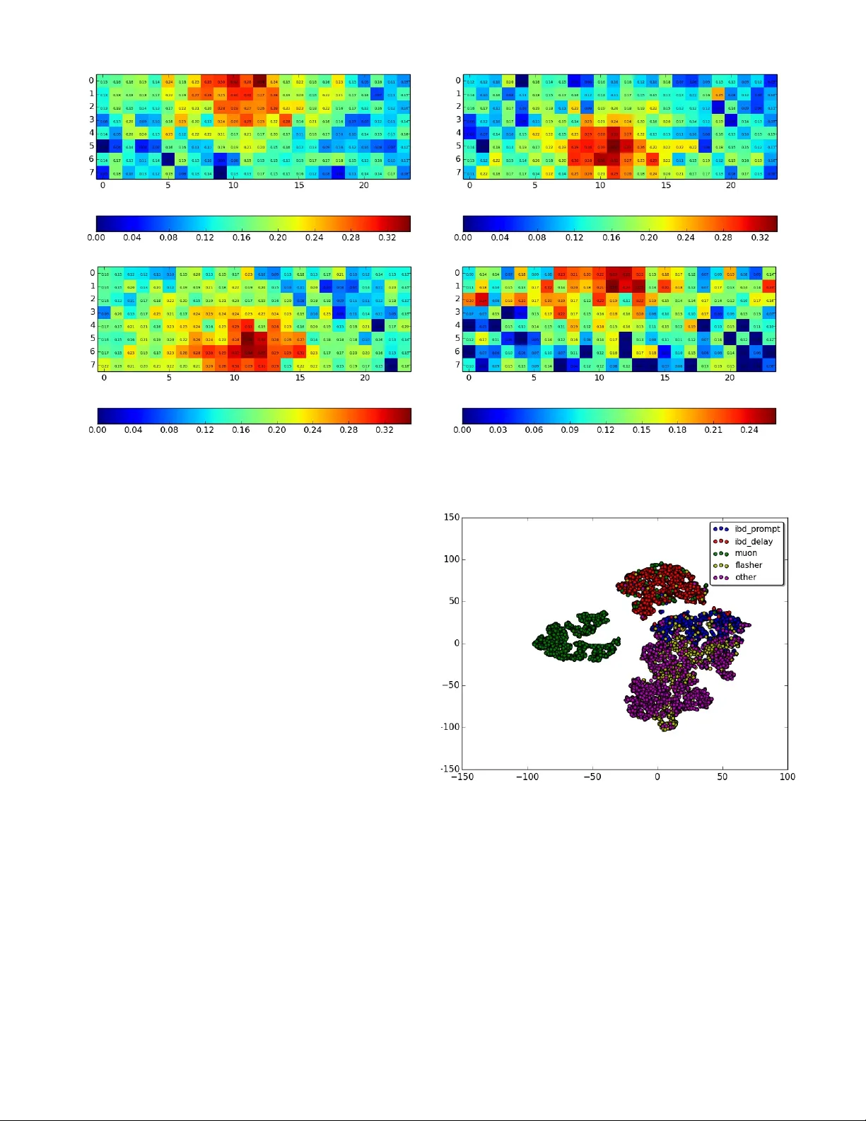
Re v ealing Fundamental Ph ysics from the Daya Bay Neutrino Experiment using Deep Neural Networks Ev an Racah ∗ , Seyoon K o † , Peter Sado wski ‡ , W ahid Bhimji ∗ , Craig T ull ∗ , Sang-Y un Oh ∗ § , Pierre Baldi ‡ , Prabhat ∗ ∗ Lawrence Berkeley Lab, Berkeley , CA Email: eracah@lbl.gov † Seoul National Uni versity , Seoul 151-747, Republic of K orea ‡ Univ ersity of California, Irvine, CA, USA § Univ ersity of California, Santa Barbara, CA, USA Abstract —Experiments in particle physics produce enormous quantities of data that must be analyzed and inter preted by teams of physicists. This analysis is often exploratory , wher e scientists are unable to enumerate the possible types of signal prior to per - forming the experiment. Thus, tools for summarizing, clustering, visualizing and classifying high-dimensional data are essential. In this work, we show that meaningful physical content can be re vealed by transforming the raw data into a learned high-le vel repr esentation using deep neural netw orks, with measur ements taken at the Daya Bay Neutrino Experiment as a case study . W e further show how con volutional deep neural networks can pro vide an effecti ve classification filter with greater than 97% accuracy across differ ent classes of physics e vents, significantly better than other machine learning approaches. Index T erms —Deep Learning, Unsupervised Learning, High- Energy Physics, A utoencoders I . I N T RO D U C T I O N The analysis of experimental data in science can be an exploratory process, where researchers do not know before- hand what the y expect to observe. This is particularly true in particle physics, where extraordinarily complex detectors are used to probe the fundamental nature of the uni verse. These detectors collect petabytes or ev en exabytes of data in order to observ e relati vely rare e vents. Analyzing this data can be a laborious process that requires researchers to carefully separate and interpret dif ferent sources of signal and noise. The Daya Bay Reactor Neutrino Experiment is designed to study anti-neutrinos produced by the Daya Bay and Ling Ao nuclear po wer plants. The experiment has successfully produced many important physics results [1], [2], [3], [4], [5] but these required significant ef fort to identify and explain the multiple sources of noise, not all of which were expected. For example, it w as found after initial data collection that a small number of the photomultiplier tubes used in the detectors spontaneously emitted light due to discharge within their base, causing so-called “flasher” events. Identifying and accounting for these flashers and other une xpected factors was critical for isolating the rare antineutrino decay e vents. T o speed up scientific research, physicists would greatly benefit from automated analyses to summarize, cluster , and visualize their data, in order to b uild an intuiti ve grasp of its structure and quickly identify flasher -like problems. V isualization and clustering are two of the primary ways that researchers use to e xplore their data. This requires trans- forming high-dimensional data (such as an image) into a 2-D or 3-D space. One common method for doing this is principle component analysis (PCA), but PCA is linear and unable to ef fectiv ely compress data that lives on a comple x manifold, such as natural images. Neural networks, on the other hand, hav e the capacity to represent very complex transformations [6]. Moreover , these transformations can be learned gi ven a sufficient amount of data. In particular, deep learning with many-layered neural networks has prov en to be an ef fective approach to learning useful representations for a variety of application domains, such as computer vision and speech recognition [7], [8]. Thus, it may provide new ways for physicists to explore their high-dimensional data. Each layer of a deep feed-forward neural netw ork computes a different non-linear representation of the input; performing e xploratory data analysis on these high-le vel representations may be more fruitful than performing the same analysis on the raw data. Furthermore, learned representations can easily be combined with e xisting tools for summarizing, clustering, visualizing and classifying data. In this work, we learn and visualize high-level represen- tations of the particle-detector data acquired by the Daya Bay Experiment. These representations are learned using both unsupervised and supervised neural network architectures. I I . R E L A T E D W O R K Finding high-level representations of ra w data is a common problem in many fields. F or example, embeddings in natural language processing attempt to find a compressed vector representation for w ords, sentences, or paragraphs where each dimension roughly corresponds to some latent feature and distance in the embedding corresponds to semantic distance (e.g. [9], [10]). In addition, for natural images, extracting features and visualizing a lo w-dimensional manifold using autoencoders is another common application [11]. These ef forts usually are applied to well-defined datasets, such as MNIST , face image datasets and SVHN. In the realm of scientific data, chemical fingerprinting is a method for representing small-molecule structures as vec- tors [12], [13]. These representations are usually engineered to capture rele vant features in the data, but an increasingly- common approach is to learn new representations from the data itself, in either a supervised or unsupervised manner . Deep neural network architectures pro vide a flexible frame work for learning these representations. Furthermore, deep learning has already been successfully applied to problems in particle physics. For example, Baldi et. al. sho wed that deep neural networks could improve exotic particle searches and showed that learned high-le vel features outperform those engineered by physicists [14]. Others ha ve applied deep neural networks to the problem of classifying particle jets from lo w-lev el detector data, using con volutional architectures and treating the detector data as images [15]. Howe ver , these ef forts hav e focused on supervised learning with simulated data; to the best of our knowledge, deep learn- ing has not been used to perform unsupervised e xploratory data analysis, directly on the raw detector measurements, with the goal of unco vering unexpected sources of signal and background noise. I I I . D A TA A Daya Bay Antineutrino Detector (AD) consists of 192 photomultiplier tubes (PMTs) arranged in a cylinder 8 PMTs high and with a 24 PMT circumference [2]. The data we use for our study is the the v alue of the charge deposit of each of the PMTs in the cylinder unwrapped into a 2D (8 “ring” x 24 “column”) array of floats. Each example is the 8x24 array for a particular e vent that set of f a trigger to be captured. For the supervised part of this analysis, and for visualizing the unsupervised results, we emplo y labels determined by the physicists from their features and threshold criteria. For full details on these selections see [2]. They label fi ve types of ev ents: “muon”, “flasher”, “IBD prompt”, “IBD delay” and a default label of “other” is applied to all other e vents. For “muon” and “flasher” ev ents we apply the physics selection on deri ved quantities held in the original data before producing our reduced data samples. In verse Beta Decay (“IBD”) labels correspond to antineutrino e vents that are the desired physics of interest and occur substantially less frequently than other ev ent types. Many stages of fairly complex analysis are used by the physicists to select these [2]. Therefore, we do not reapply that selection but instead use an index output from their analyses to tag ev ents. Muon labelled e vents are relati vely straightforward to clus- ter or learn, while flasher and IBD events inv olve non- linear functions and complex transformations. Furthermore, the physicists’ selections for these events make use of some information that is not a vailable to our analysis, such as times between events and with respect to external muon detectors. I V . M E T H O D S Giv en a set of detector images, we aim to find a vector representation, V ∈ R n of each image, where n corresponds to the number of features to be learned. The features are task- specific — they are optimized either for class-prediction or reconstruction — but in both cases we expect the learned representation to capture high-le vel information about the data. By transforming the ra w data into these high-lev el represen- tations, we aim to provide physicists with more interpretable clusterings and visualizations, so that the y may uncov er unex- pected sources of signal and background. T o learn ne w representations, we use both supervised and unsupervised con volutional neural networks. These methods are described in more detail belo w . As a qualitativ e assessment of the learned representations, we use t-Distributed Stochastic Neighbor Embedding (t-SNE) [16], which maps n-dimensional data to 2 or 3 dimensions and makes sure points close together in the high n-dimensional space are also close together in the lower dimensional embedding. A. Supervised Learning with Con volutional Neur al Networks A con v olutional neural network (CNN) is a particular neural network architecture that captures our intuition about local structure and translational in variance in images [7]. W e em- ploy CNNs in this work because the data captured by the antineutrino detectors are essentially 2-D images. Most CNNs hav e several con volutional and pooling layers followed by one or more fully connected layers that use the features learned from those layers to perform typical classification or regression tasks. B. Unsupervised Learning with Con volutional A utoencoders An autoencoder [17], [18] is a neural network where the target output is exactly the input. It usually consists of an encoder , which consists of one or more layers that transform the input into a feature vector at the output of the middle layer (often called bottleneck layer or hidden layer), and a decoder , which usually contains se veral layers that attempt to reconstruct the hidden layer output back to the input. When the autoencoder architecture includes a hidden layer output with dimensionality smaller than that of the input (undercomplete), it must learn ho w to compress and reconstruct examples from the training data. It has been sho wn that undercomplete autoen- coders are equiv alent to nonlinear PCA [19]. In addition, there exist autoencoders that hav e hidden layer ouputs of higher dimension than the those of the inputs (ov ercomplete) that use other constraints to prevent the network from learning an identity function [11], [20], [21]. W e use undercomplete autoencoders due to their simplicity and as an exploratory first step to see if we can indeed extract low dimensional features from this sensor data, while still taking nonlinearity into account. A con volutional autoencoder is an autoencoding architec- ture that includes conv olutional layers. The encoding portion typically consists of con volutional and max-pooling layers followed by fully-connected hidden layers (including a “bottle- neck” layer) and then decon volutional (and unpooling) layers, usually one for each con volutional and pooling layer [22]. layer type filter size filters stride activ ation 1 con v 3 × 3 71 1 tanh 2 pool 2 × 2 1 2 max 3 con v 2 × 2 88 1 tanh 4 pool 2 × 2 1 2 max 5 fc 1 × 5 26 1 tanh 6 fc 1 × 1 5 1 softmax T ABLE I: Architecture of the supervised CNN layer type filter size filters stride pad activ ation 1 conv 5 × 5 16 1 2x2 RELU [7] 2 pool 2 × 2 1 2 0 max 3 conv 3 × 3 16 1 1 × 0 RELU 4 pool 2 × 2 1 2 0 max 5 fc 2 × 5 10 1 0 RELU 6 decon v 2 × 4 16 2 0 None 7 decon v 2 × 5 16 2 0 None 8 decon v 2 × 4 1 2 0 None T ABLE II: Architecture of the conv olutional autoencoder While some authors [23] have shown success with using decon volutional and unpooling layers in reconstruction, we solely use transposed conv olutional layers due to software constraints. Moreov er , there has been work with con volutional generativ e models that sho ws success in using just fractionally strided conv olutional layers and no unpooling layers [24]. V . I M P L E M E N TA T I O N W e performed our analysis on Edison and Cori, tw o Cray XC computing systems at the National Energy Research Scientific Computing Center (NERSC). A. Pr eprocessing For training and testing data, we used an equal number of examples from each of the fi ve physics classes. Because the muon charge deposit values are much higher than some of the other ev ents’ charge deposits, we apply a natural log transform to each v alue in the 8x24 image. For the supervised CNN, we also cyclically permute the columns, so the column containing the lar gest v alued element in the entire array is in the center (12th column). This is done to prev ent areas of interest from being located on the edges of the array (gi ven the data is an array from an unwrapped cylinder). B. Supervised Learning with CNN T o help examine if there were learnable patterns in the data, we implemented a supervised con volutional neural net. The architecture of the CNN is specified in T able I. W e trained the network on 45,000 examples using stochastic gradient descent. W e then classified 15,000 test examples using the trained model. The classification performance was compared with k- nearest neighbor classifiers and support vector machines. C. Unsupervised Learning with Con volutional A utoencoders For the conv olutional autoencoder , we use the architecture specified in T able II, using sum of squared error as the loss function. The con volutional autoencoder was trained using gra- dient descent with a learning rate of 0.0005 and a momentum Measure IBD IBD Muon Flasher Other and Method prompt delay F 1 -score k-NN 0.775 0.954 0.996 0.784 0.806 SVM 0.846 0.962 0.996 0.895 0.885 CNN 0.891 0.974 0.997 0.951 0.928 Accuracy k-NN 0.950 0.990 0.998 0.891 0.896 SVM 0.966 0.992 0.998 0.947 0.938 CNN 0.977 0.995 0.999 0.974 0.962 T ABLE III: Classifier performance for different ev ents Fig. 2: t-SNE reduction of representation learned on the last fully connected layer of CNN. Representati ve examples from the clusters immediately belo w the labels A and B and to the left of C are shown in figure 1a – 1d coefficient of 0.9. W e trained the netw ork on 31,700 training examples and tested it on 7900 test examples. V I . R E S U LTS A. Supervised Learning with CNN 1) Results: The classification classwise F 1 -scores and clas- sification accuracies of k-nearest neighbor , support v ector ma- chine, and the CNN architecture on the test set are summarized in T able III. W e also used t-SNE [16] to visualize the features learned for the supervised conv olutional neural network. Fig- ure 2 shows the t-SNE visualization of the outputs from the last fully connected layer of the CNN. This visualization sho ws in two dimensions ho w the each example is clustered in the 26-dimensional feature space learned by the network. W e also show , in Figures 1a and 1b, e xample PMT charges of different types of ev ents that are in clusters in the t-SNE clustering (Figure 2) that contain a mix of labels near each other , as well as examples contained in well separated clusters in Figures 1c and 1d. These examples are visualizations of the 8x24 arrays after preprocessing. As described in the preprocessing section, the value of each element in the array is the ra w charge deposit as measured by the PMT at the time of the trigger transformed by a natural log and then divided by a scale factor of 10 to ensure values between 0 and 1. (a) An IBD delay event in cluster A (b) An IBD prompt event in cluster A (c) An IBD delay event in cluster C (d) An IBD prompt event in the blue cluster belo w the letter B Fig. 1: Representati ve examples of v arious IBD e vents in the clusters labeled in Figure 2. 2) Interpr etation: Our results suggest that there are patterns in the Daya Bay data that can be uncovered by machine learning techniques without knowledge of the underlying physics. Specifically , we were able to achiev e high accuracy on classification of the Daya Bay events using only the spatial pattern of the char ge deposits. In contrast, the physicists used the time of the events and prior physics knowledge to perform classification. In addition, our results suggest that deep neural networks were better than other techniques at classifying the images and thus finding patterns in the data. as shown in T able III. Our CNN architecture had the highest F 1 -score and accuracy for all ev ent types. In particular , it showed significantly higher performance on classes “IBD prompt” and “flasher”. Not only did the supervised CNN perform better in classifying the data then other shallower ML techniques, but it also discovered features in the data that helped cluster it into fairly distinct groups as shown in Figure 2. W e can further in vestigate the raw images within the clusters formed by t-SNE. For example, in Figures 1a and 1b the CNN has identified a particularly distincti ve charge pattern common to both images. Specifically , both images have the same range of v alues and ha ve a very similar shape. Though the patterns happen at dif ferent parts of the image, they are roughly the same and it is not surprising that the CNN picked up on this translation in v ariant pattern. These are labeled as different types because prompt events have a large range of charge patterns, some of which v ery closely resemble delay ev ents. The standard physics analysis is able to resolve these only by using the time coincidence of delay ev ents happening Fig. 3: t-SNE representation of features learned by the con vo- lutional autoencoder within 200 microseconds after prompt e vents, while the neural network solely has charge pattern information. Future work in volving these features may help solv e this, but it is nev er- theless encouraging that the network w as able to hone in on the geometric pattern. Figures 1c and 1d, on the other hand, show images from more distinct prompt and delay clusters, respectiv ely , illustrating that prompt e vents deposit less energy in the detector on a verage as shown by the different range of values in the two images. Such clustering suggests that, with (a) Example of an “IBD delay” e vent (b) Example of an “IBD prompt” e vent Fig. 4: Ra w e vent image (top row) and con volutional autoencoder reconstructed event image (bottom ro w). help from ground truth labeling, deep learning techniques can discov er informative features and thus find structure in raw physics inputs. Because such patterns in the data exist and can be learned, this suggests that unsupervised learning also has the potential to discov er these patterns without needing ground truth labeling. B. Unsupervised learning with Con volutional A utoencoder 1) Results: For the con volutional autoencoder , we present the t-SNE visualization of the 10 features learned by the network in figure 3. T o show how informativ e the feature vector that the netw ork learned is, we also show several ev ent images and their reconstruction by the autoencoder in Figures 4a and 4b. More informativ e features that are learned correspond to more accurate reconstructions because the 10 features ef fectiv ely give the network the “ingredients” it needs to the reconstruct the input 8x24 structure. 2) Interpr etation: The con volutional autoencoder is de- signed to reconstruct PMT images and so it learns dif ferent features than the supervised CNN which is attempting to classify based on the training labels. Therefore, the t-SNE clustering for this part of the study (in Figure 3) is quite different from that in the supervised section. Nev ertheless, we were able to obtain well defined clusters without using any physics knowledge. Specifically , there is a very clearly separated cluster that can be identified with the labelled muons, and also a fairly clear separation between “IBD delay” and other e vents. W e even achie ve some separation between “IBD prompt” and “other” backgrounds which, as mentioned abov e, is mainly achiev ed in the default physics analysis only by incorporating additional information of the time between prompt and delayed e vents. By looking at the reconstructed images, we can see the au- toencoder was able to filter out the input noise and reconstruct the important shape of dif ferent e vent types. For example, in Figure 4a, the shape of the char ge pattern is reconstructed extremely accurately , which shows that the 10 learned features from the autoencoder are very informative for “IBD delay” ev ents. In Figure 4b, salient and distinct aspects, lik e the high charge regions on the right side and the low regions on the left, of the more challenging “IBD prompt” ev ents are also reconstructed well. As further work, it would be desirable to obtain better separation between “flasher” and “other” e vents. Therefore we intend to continue to tailor the conv olutional autoencoder approach to this application by considering input transformations that take into account the e xperiment geome- try , variable resolution images, and alternativ e construction of con volutional filters, as well as more data and full parameter optimization of the number of filters and the size of the feature vector . V I I . C O N C L U S I O N S In this work we have applied for the first time unsupervised deep neural nets within particle physics and have shown that the network can successfully identify patterns of physics interest. As future work we are collaborating with physicists on the experiment to in vestigate in detail the v arious clusters formed by the representation to determine what interesting physics is captured in them be yond the initial labelling. W e also plan to incorporate such visualizations into the monitoring pipeline of the experiment. Such unsupervised techniques could be utilized in a generic manner for a wide variety of particle physics experiments and run directly on the raw data pipeline to aid in trigger (filter) decisions or in ev aluating data quality , or to dis- cov er new instrument anomalies (such as flasher ev ents). The use of unsupervised learning to identify such features is of considerable interest within the field as it can potentially sav e considerable time required to hand-engineer features to identify such anomalies. W e ha ve also demonstrated the superiority of conv olutional neural networks compared to other supervised machine learn- ing approaches for running directly on raw particle physics instrument data. This of fers the potential for use as fast selec- tion filters, particularly for other particle physics experiments that ha ve many more channels and approach e xabytes of raw data such as those at the current Lar ge Hadron Collider (LHC) and planned HL-LHC at CERN [25]. Our analysis in this paper used the labels determined from an existing physics analysis and therefore the selection accurac y is upper bounded by that of the physics analysis. Many other particle physics experiments, howe ver , have reliable simulated data which could be used with the approaches in this paper to better the selection accuracy achieved with those experiments’ current analyses. In conclusion, we have demonstrated how deep learning can be applied to re veal physics directly from raw instrument data ev en with unsupervised approaches, and therefore that these techniques of fer considerable potential to aid the fundamental discov eries of future particle physics experiments. A C K N O W L E D G M E N T S The authors gratefully acknowledge the Daya Bay Collab- oration for access to their e xperimental data and many useful discussions, and specifically Y asuhiro Nakajima for the dataset labels, and physics background details. This research was conducted using neon, an open source library for deep learning from Nervana Systems. This research used resources of the National Energy Research Scientific Computing Center , a DOE Office of Science User Facility supported by the Office of Science of the U.S. Department of Energy under Contract No. DE-A C02-05CH11231. This work was supported by the Director , Office of Science, Office of Advanced Scientific Computing Research, Applied Mathematics program of the U.S. Department of Energy under Contract No. DE-A C02-05CH11231. S. Ko was supported by Basic Science Research Program through the National Research Foundation of K orea (NRF) grants funded by the Korea gov ernment (MSIP) (Nos. 2013R1A1A1057949 and 2014R1A4A1007895). R E F E R E N C E S [1] F . P . A. et al. [Daya Bay Collaboration], “Observation of electron- antineutrino disappearance at Daya Bay , ” Physical Review Letters , vol. 108, no. 17, p. 171803, 2012. [2] ——, “Improved measurement of electron antineutrino disappearance at Daya Bay , ” Chinese Physics C , vol. 37, no. 1, p. 011001, 2013. [3] ——, “Search for a light sterile neutrino at Daya Bay , ” Physical Review Letters , vol. 113, no. 14, p. 141802, 2014. [4] ——, “Independent measurement of the neutrino mixing angle θ 13 via neutron capture on hydrogen at Daya Bay , ” Physical Review D , vol. 90, no. 7, p. 071101, 2014. [5] ——, “ A ne w measurement of antineutrino oscillation with the full detector configuration at Daya Bay , ” arXiv pr eprint arXiv:1505.03456 , 2015. [6] K. Hornik, M. Stinchcombe, and H. White, “Multilayer feedforward networks are uni versal approximators, ” Neural Netw . , vol. 2, no. 5, pp. 359–366, Jul. 1989. [Online]. A vailable: http://dx.doi.org/10.1016/ 0893- 6080(89)90020- 8 [7] A. Krizhevsky , I. Sutskever , and G. E. Hinton, “Imagenet classification with deep conv olutional neural networks, ” in Advances in neural infor- mation pr ocessing systems , 2012, pp. 1097–1105. [8] G. Hinton, L. Deng, D. Y u, G. E. Dahl, A.-r . Mohamed, N. Jaitly , A. Senior, V . V anhoucke, P . Nguyen, T . N. Sainath et al. , “Deep neural networks for acoustic modeling in speech recognition: The shared views of four research groups, ” Signal Processing Ma gazine, IEEE , v ol. 29, no. 6, pp. 82–97, 2012. [9] Q. V . Le and T . Mikolov , “Distributed representations of sentences and documents, ” CoRR , vol. abs/1405.4053, 2014. [Online]. A vailable: http://arxiv .org/abs/1405.4053 [10] R. Kiros, Y . Zhu, R. Salakhutdino v , R. S. Zemel, A. T orralba, R. Urtasun, and S. Fidler, “Skip-thought vectors, ” CoRR , vol. abs/1506.06726, 2015. [Online]. A vailable: http://arxiv .org/abs/1506.06726 [11] D. P . Kingma and M. W elling, “ Auto-encoding variational bayes, ” arXiv pr eprint arXiv:1312.6114 , 2013. [12] A. Lusci, G. Pollastri, and P . Baldi, “Deep architectures and deep learning in chemoinformatics: The prediction of aqueous solubility for drug-like molecules, ” Journal of Chemical Information and Modeling , vol. 53, no. 7, pp. 1563–1575, 2013, pMID: 23795551. [Online]. A vailable: http://dx.doi.org/10.1021/ci400187y [13] D. K. Duvenaud, D. Maclaurin, J. Aguilera-Iparraguirre, R. G ´ omez- Bombarelli, T . Hirzel, A. Aspuru-Guzik, and R. P . Adams, “Con volutional networks on graphs for learning molecular fingerprints, ” CoRR , vol. abs/1509.09292, 2015. [Online]. A vailable: http://arxiv .org/abs/1509.09292 [14] P . Baldi, P . Sadowski, and D. Whiteson, “Searching for e xotic particles in high-energy physics with deep learning, ” Natur e communications , v ol. 5, 2014. [15] L. de Oli veira, M. Kagan, L. Mack ey , B. Nachman, and A. Schwartzman, “Jet-images–deep learning edition, ” arXiv pr eprint arXiv:1511.05190 , 2015. [16] L. V an der Maaten and G. Hinton, “V isualizing data using t-sne, ” Journal of Machine Learning Researc h , vol. 9, no. 2579-2605, p. 85, 2008. [17] Y . Bengio, P . Lamblin, D. Popovici, H. Larochelle et al. , “Greedy layer-wise training of deep networks, ” Advances in neural information pr ocessing systems , vol. 19, p. 153, 2007. [18] Y . Bengio, “Learning deep architectures for ai, ” F oundations and trends in Machine Learning , vol. 2, no. 1, pp. 1–127, 2009. [19] M. A. Kramer , “Nonlinear principal component analysis using autoas- sociativ e neural networks, ” AIChE journal , vol. 37, no. 2, pp. 233–243, 1991. [20] P . V incent, H. Larochelle, Y . Bengio, and P .-A. Manzagol, “Extract- ing and composing rob ust features with denoising autoencoders, ” in Pr oceedings of the 25th international conference on Machine learning . A CM, 2008, pp. 1096–1103. [21] S. Rifai, P . V incent, X. Muller, X. Glorot, and Y . Bengio, “Contractiv e auto-encoders: Explicit in variance during feature e xtraction, ” in Pr oceed- ings of the 28th international confer ence on machine learning (ICML- 11) , 2011, pp. 833–840. [22] V . Dumoulin and F . V isin, “ A guide to con volution arithmetic for deep learning, ” arXiv pr eprint arXiv:1603.07285 , 2016. [23] J. Zhao, M. Mathieu, R. Goroshin, and Y . Lecun, “Stacked what-where auto-encoders, ” arXiv pr eprint arXiv:1506.02351 , 2015. [24] A. Radford, L. Metz, and S. Chintala, “Unsupervised representation learning with deep con volutional generati ve adversarial networks, ” arXiv pr eprint arXiv:1511.06434 , 2015. [25] A. Collaboration, “Letter of intent for the phase-ii upgrade of the atlas experiment, ” CERN Document Server CERN-LHCC-2012-022 , 2012.