Inverse Reinforcement Learning via Deep Gaussian Process

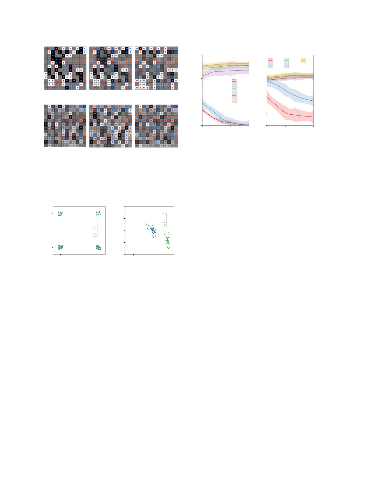
In verse Reinf orcement Learning via Deep Gaussian Process Ming Jin ∗ EECS, UC Berkeley , USA jinming@berkeley .edu Andreas Damianou † Amazon.com, Cambridge, UK damianou@amazon.com Pieter Abbeel EECS, UC Berkeley , USA pabbeel@berkeley .edu Costas Spanos EECS, UC Berkeley , USA spanos@berkeley .edu Abstract W e propose a new approach to in verse rein- forcement learning (IRL) based on the deep Gaussian process (deep GP) model, which is capable of learning complicated re ward struc- tures with few demonstrations. Our model stacks multiple latent GP layers to learn ab- stract representations of the state feature space, which is linked to the demonstrations through the Maximum Entropy learning framew ork. In- corporating the IRL engine into the nonlinear latent structure renders existing deep GP infer - ence approaches intractable. T o tackle this, we dev elop a non-standard variational approxima- tion framework which extends previous infer- ence schemes. This allows for approximate Bayesian treatment of the feature space and guards against overfitting. Carrying out rep- resentation and inv erse reinforcement learn- ing simultaneously within our model outper- forms state-of-the-art approaches, as we demon- strate with experiments on standard bench- marks (“object world”,“highway dri ving”) and a new benchmark (“binary w orld”). 1 INTR ODUCTION The problem of inv erse reinforcement learning (IRL) is to infer the latent re ward function that the agent subsumes by ∗ This research is funded by the Republic of Singapore’ s National Research Foundation through a grant to the Berkeley Education Alliance for Research in Singapore (BEARS) for the Singapore-Berkele y Building Efficienc y and Sustainability in the T ropics (SinBerBEST) Program. BEARS has been estab- lished by the Uni versity of California, Berkele y as a center for intellectual excellence in research and education in Singapore. † W ork done while this author was at the Uni versity of Sheffield. observing its demonstrations or trajectories in the task. It has been successfully applied in scientific inquiries, e.g., animal and human behavior modeling (Ng et al., 2000), as well as practical challenges, e.g., navigation (Ratliff et al., 2006; Abbeel et al., 2008; Ziebart et al., 2008) and intelligent building controls (Barrett and Linder, 2015). By learning the rew ard function, which provides the most succinct and transferable definition of a task, IRL has en- abled adv ancing the state of the art in the robotic domains (Abbeel and Ng, 2004; K olter et al., 2007). Previous IRL algorithms treat the underlying re ward as a linear (Abbeel and Ng, 2004; Ratliff et al., 2006; Ziebart et al., 2008; Syed and Schapire, 2007; Ratliff et al., 2009) or non-parametric function (Levine et al., 2010; 2011) of the state features. Main formulations within the linearity category include maximum mar gin (Ratliff et al., 2006), which presupposes that the optimal reward function leads to maximal difference of expected re ward between the demonstrated and random strategies, and feature expecta- tion matching (Abbeel and Ng, 2004; Syed et al., 2008), based on the observation that it suffices to match the feature expectation of a policy to the expert in order to guarantee similar performances. The reward function can be also regarded as the parameters for the policy class, such that the likelihood of observing the demonstrations is maximized with the true rew ard function, e.g., the max- imum entropy approach (Ziebart et al., 2008). As the representation power is limited by the linearity assumption, nonlinear formulations (Le vine et al., 2010) are proposed to learn a set of composite features based on logical conjunctions. Non-parametric methods, pioneered by (Levine et al., 2011) based on Gaussian Processes (GPs) (Rasmussen, 2006), greatly enlarge the function space of latent re ward to allo w for non-linearity , and hav e been shown to achie ve the state of the art performance on benchmark tests, e.g., object world and simulated high- way driving (Abbeel and Ng, 2004; Syed and Schapire, 2007; Levine et al., 2010; 2011). Nev ertheless, the heavy reliance on predefined or handcrafted features becomes a bottleneck for the existing methods, especially when the complexity or essence of the re ward can not be captured by the given features. Finding such features automatically from data would be highly desirable. In this paper, we propose an approach which performs feature and in verse reinforcement learning simultaneously and coherently within the same model by incorporating deep learning. The success of deep learning in a wide range of domains has drawn the community’ s attention to its structural advantages that can improve learning in complicated scenarios, e.g., Mnih et al. (2013) re- cently achieved a deep reinforcement learning (RL) break- through. Nev ertheless, most deep models require massiv e data to be properly trained and can become impractical for IRL. On the other hand, deep Gaussian processes (deep GPs) (Damianou and Lawrence, 2013; Damianou, 2015) not only can they learn abstract structures with smaller data sets, but they also retain the non-parametric proper- ties which Le vine et al. (2011) demonstrated as important for IRL. A deep GP is a deep belief netw ork comprising a hierar - chy of latent v ariables with Gaussian process mappings between the layers. Analogously to how gradients are propagated through a standard neural network, deep GPs aim at propagating uncertainty through Bayesian learning of latent posteriors. This constitutes a useful property for approaches in volving stochastic decision making and also guards against ov erfitting by allowing for noisy fea- tures. Ho wev er , previous methodologies employed for approximate Bayesian learning of deep GPs (Damianou and Lawrence, 2013; Hensman and Lawrence, 2014; Bui et al., 2015; Mattos et al., 2016) fail when diver ging from the simple case of fixed output data modeled through a Gaussian regression model. In particular, in the IRL setting, the re ward (output) is only re vealed through the demonstrations, which is guided by the policy giv en by the reinforcement learning (Damianou, 2015). The main contributions of our paper are belo w . • W e extend the deep GP framework to the IRL do- main (Fig. 1), allo wing for learning latent rewards with more complex structures from limited data. • W e deriv e a variational lo wer bound on the marginal log likelihood using an innov ativ e definition of the vari ational distributions. This methodological contri- bution enables Bayesian learning in our model and can be applied to other scenarios where the observ a- tion layer’ s dynamics cause similar intractabilities. • W e compare the proposed deep GP for IRL with existing approaches in benchmark tests as well as newly defined tests with more challenging re wards. T able 1: Summary of notations. t time step t ∈ { 1 , 2 , · · · , T } h index of demonstrations h ∈ { 1 , · · · , H } s, a state s ∈ S , action a ∈ A γ RL discount factor , γ ∈ (0 , 1) r re ward vector for all states s ∈ S r ( · ) rew ard function for states S 7→ R Q ( · ) Q-value function S × A 7→ R Q variational distrib ution V ( · ) state v alue function S 7→ R π , ˆ π , π ∗ policy S 7→ A , and the corresponding estimated and optimal versions X m 0 -dimensional feature matrix for |S | = n discrete states, X ∈ R n,m 0 x i , x m features for i th state, [ X ] i, : = x i , the m th feature for all states, [ X ] : ,m = x m k θ cov ariance function parametrized by θ K X , X cov ariance matrix, [ K X , X ] i,j = k θ ( x i , x j ) B latent state matrix with m 1 -dimensional features, B ∈ R n,m 1 D B with Gaussian noise, D ∈ R n,m 1 W , Z inducing inputs, W ∈ R K,m 0 , Z ∈ R K,m 1 V , f inducing outputs, V ∈ R K,m 1 , f ∈ R K tilde ˜ mean of the corresponding variable distri- bution, e.g., ˜ f , ˜ v , ˜ D In the following, we re view the problem of inv erse re- inforcement learning (IRL). The list of notations used throughout the paper is summarized in T able 1. 1.1 In verse Reinfor cement Learning The Marko v Decision Process (MDP) is characterized by {S , A , T , γ , r } , which represents the state space, ac- tion space, transition model, discount factor , and rew ard function, respectiv ely . T ake robot navigation as an example. The goal is to trav el to the goal spot while a voiding stairwells. The state describes the current location and heading. The robot can choose actions from going forward or backward, turning left or right. The transition model specifies p ( s t +1 | s t , a t ) , i.e., the probability of reaching the next state giv en the current state and action, which accounts for the kinematic dynamics. The reward is +1 if it achie ves the goal, -1 if it ends up in the stairwell, and 0 otherwise. The discount factor , γ , is a positiv e number less than 1, e.g., 0.9, to discount the future rew ards. The optimal policy is then giv en by maximizing the expected rew ard, i.e., π ∗ = arg min π E " ∞ X t =0 γ t r ( s t ) | π # . (1) Figure 1: Left: The proposed deep GP model for IRL. The tw o layers of GPs are stack ed to generate the latent re ward r , which is input to the reinforcement learning (RL) engine to produce an optimal control policy and demonstrations. X denotes the initial feature representation of states. Right: Illustration of DGP-IRL augmented with inducing outputs f , V and corresponding inputs Z , W . The IRL task is to find the rew ard function r ∗ such that the induced optimal policy matches the demonstra- tions, giv en {S , A , T , γ } and M = { ζ 1 , ..., ζ H } , where ζ h = { ( s h, 1 , a h, 1 ) , ..., ( s h,T , a h,T ) } is the demonstration trajectory , consisting of state-action pairs. Under the lin- earity assumption , the feature representation of states forms the linear basis of re ward, r ( s ) = w > φ ( s ) , where φ ( s ) : S 7→ R m 0 is the m 0 -dimensional mapping from the state to the feature vector . From this definition, the expected r ewar d for policy π is gi ven by: E " ∞ X t =0 γ t r ( s t ) | π # = w > E " ∞ X t =0 γ t φ ( s t ) | π # where µ ( π ) = E [ P ∞ t =0 γ t φ ( s t ) | π ] is the feature expec- tation for policy π . The re ward parameter w ∗ is learned such that w ∗> µ ( π ∗ ) ≥ w ∗> µ ( π ) , ∀ π (2) a prev alent idea that appears in the maximum mar gin plan- ning (MMP) (Ratliff et al., 2006) and feature expectation matching (Syed and Schapire, 2007). Motiv ated by the perspective of expected rew ard that parametrizes the policy class, the maximum entropy (Max- Ent) model (Ziebart et al., 2008) considers a stochastic de- cision model, where the optimal policy randomly chooses the action according to the associated rew ard: p ( a | s ) = exp { Q ∗ ( s, a ; r ) − V ∗ ( s ; r ) } (3) where V ( s ; r ) = log P a exp( Q ( s, a ; r )) follows the Bellman equation, Q ( s, a ; r ) and V ( s ; r ) are measures of ho w desirable are the corresponding state s and state- action pair ( s, a ) under rewards r . In principle, for a giv en state s , the best action corresponds to the highest Q-value, which represents the “desirability” of the action. Assuming independence among state-action pairs from demonstrations, the likelihood of the demonstration cor- responds to the joint probability of taking a sequence of actions a i,t under states s h,t according to the Bellman equation: p ( M| r ) = H Y h =1 T Y t =1 p ( a h,t | s h,t ) = exp H X h =1 T X t =1  Q ( s h,t , a h,t ; r ) − V ( s h,t ; r )  ! . (4) Though directly o ptimizing the above criteria with respect to r is possible, it does not lead to generalized solutions transferrable in a new test case where no demonstrations are av ailable; hence, we need a “model” of r . MaxEnt as- sumes linear structure for rewards, while GPIRL (Le vine et al., 2011) uses GPs to relate the states to rew ards. In Section 2.1, we will give a brief ov erview of GPs and GPIRL. 2 The Model In this section, we start by discussing the re ward model- ing through Gaussian processes (GPs) following (Le vine et al., 2011), proceed to incorporate the representation learning module as additional GP layers, then de velop our variational training framework and, finally , develop the transfer between tasks. 2.1 Gaussian Process Reward Modeling W e consider the setup of discr etizing the world into n states. Assume that observed state-action pairs (demon- strations) M = { ζ 1 , . . . , ζ h } are generated by a set of m 0 − dimensional state features X ∈ R n,m 0 through the reward function r . Throughout this paper we de- note points (rows of a matrix) as [ X ] i, : = x i , fea- tures (columns) as [ X ] : ,m = x m and single elements as [ X ] i,m = x m i . In this modeling frame work, the re ward function r plays the role of an unknown mapping, thus we wish to treat it as latent and keep it flexible and non-linear . Therefore, we follo w (Levine et al., 2011) and model it with a zero-mean GP prior (Rasmussen, 2006): r ∼ G P (0 , k θ ( x i , x j )) , where k θ denotes the covariance function, e.g. k θ ( x i , x j ) = σ 2 k e − ξ 2 ( x i − x j ) > ( x i − x j ) , θ = { σ k , ξ } . Giv en a finite amount of data, this induces the proba- bility r | X , θ ∼ N ( 0 , K XX ) , where r , r ( X ) and the cov ariance matrix is obtained by [ K XX ] i,j = k θ ( x i , x j ) . The GPIRL training objectiv e comes from integrating out the latent rew ard: p ( M| X ) = Z p ( M| r ) p ( r | X , θ ) d r (5) and maximizing ov er θ , which we drop from our expres- sions from now on. The abo ve integral is intractable, because p ( M| r ) has the complicated expression of (4) (this is in contrast to the tranditional GP regression where M| r is a Gaussian or other simple distrib ution). This can be alle viated using the approximation of (Levine et al., 2011). W e will describe this approximation in the next section, as it is also used by our approach. Notice that all latent function instantiations are linked through a joint multiv ariate Gaussian. Thus, prediction of the function v alue r ∗ = r ( x ∗ ) at a test input x ∗ is found through the conditional r ∗ | r , X , x ∗ ∼ N  K x ∗ X K − 1 XX r , k x ∗ x ∗ − K x ∗ X K − 1 XX K Xx ∗  As can be seen, the prediction r ( x ∗ ) is reliant on the ef- fectiveness of featur e repr esentation : states with features close in Euclidean distance are assumed to be associated with similar re wards. This motiv ates our nov el deep GP- IRL method which is obtained by considering additional layers, as we will describe next. 2.2 Incorporating the Representation Learning Layers The traditional model-based IRL approach is to learn the latent re ward r (operating on fixed state features X ) that best explains the demonstrations M . In this paper we wish to additionally and simultaneously uncover a highly descriptiv e state feature representation. T o achiev e this, we introduce a latent state feature representation B =  b 1 , ..., b m 1  ∈ R n,m 1 . B constitutes the instantiations of an introduced function b which is learned as a non- linear GP transformation from X . T o account for noise we further introduce D as the noisy versions of B , i.e., d m i = b m i +  ,  ∼ N (0 , λ − 1 ) . Importantly , rather than performing two steps of learn- ing separately (for the GPs on r and on b ), we nest them into a single objectiv e function, to maintain the flow of information during optimization. This results in a deep GP whose top layers perform representation learning and lower layers perform model-based IRL. Fig. 1 outlines our model, Deep Gaussian Process for In verse Reinforce- ment Learning ( DGP-IRL ). By using x m to represent the m -th column of X , and similarly for D , B the full generativ e model is written as follows: p ( M , r , D , B | X ) = p ( M| r ) | {z } IRL p ( r | D ) | {z } G P ( 0 ,k r ( d i , d j )) p ( D | B ) | {z } Gaussian noise p ( B | X ) | {z } G P ( 0 ,k b ( x i , x j )) = e P H h =1 P T t =1  Q ( s h,t ,a h,t ; r ) − V ( s h,t ; r )  N ( r | 0 , K DD ) m 1 Y m =1 N ( d m | b m , λ − 1 I ) N ( b m | 0 , K XX ) , (6) where the IRL term p ( M| r ) takes the form of (4) as suggested by Ziebart et al. (2008). K XX and K DD are the cov ariance matrices in each layer, constructed with cov ariance functions k b and k r respectiv ely . Compared to GPIRL the proposed framew ork has substantial gain in flexibility by introducing the abstract representation of states in the hidden layers B , D . Note that the model in Fig. 1 can be extended in depth by introducing additional hidden layers and connecting them with additional GP mappings; it is only for illustration simplicity that we base our deriv ation on the two layered structure. W e can compress the statistical po wer of each genera- tiv e layer into a set of auxiliary variables within a sparse GP frame work (Snelson and Ghahramani, 2005). Specifi- cally , we introduce inducing outputs and inputs , denoted by f ∈ R K and Z ∈ R K,m 1 respectiv ely for the lower layer and by V ∈ R K,m 1 and W ∈ R K,m 0 for the top layer (as in Fig. 1). The inducing outputs and inputs are related with the same GP prior appearing in each layer . For e xample, f | Z ∼ N ( 0 , K ZZ ) with K ZZ = k r ( Z , Z ) . By relating the original and inducing variables through the conditional Gaussian distrib ution, the auxiliary v ari- ables are learned to be sufficient statistics of the GP . The augmented model, shown in Fig. 1, has the following definition: p ( M , r , f , B , D , V | X , Z , W ) (7) = p ( M| r ) p ( r | f , D , Z ) p ( f | Z ) p ( D | B ) p ( B | V , X , W ) = e P H h =1 P T t =1  Q ( s h,t ,a h,t ; r ) − V ( s h,t ; r )  · N ( r | K DZ K − 1 ZZ f , Σ r ) N ( f | 0 , K ZZ ) · m 1 Y m =1 N ( d m | b m , λ − 1 I ) N ( b m | K XW K − 1 WW v m , Σ B ) where we adopt the Fully Independent T raining Condi- tional (FITC) to preserve the exact variances in Σ B = diag  K XX − K XW K − 1 WW K WX  , and the Determinis- tic T raining Conditional (DTC) (Qui ˜ nonero-Candela and Rasmussen, 2005) in Σ r = 0 as in GPIRL to facilitate the integration of r in the training objective (see next section). In the following, we will omit the inducing inputs W , Z in the conditions, with the con vention to treat them as model parameters (Damianou and Lawrence, 2013; Damianou, 2015; Kandemir, 2015b). By selecting K  n the com- plexity reduces from O ( n 3 ) to O ( nK 2 ) . While DGP-IRL resolves the case when the outputs hav e complex depen- dencies with the latent layers, the training of the model based on v ariational inference requires gradients for the parameters, as in backpropagation, whose conv ergence can be improv ed by leveraging adv ancements in deep learning. Additionally , in DGP-IRL , the role of auxiliary variables goes further than just introducing scalability . Indeed, as we shall see next, the auxiliary variables play a distinct role in our model, by forming the base of a variational framew ork for Bayesian inference. 2.3 V ariational Inference W e wish to optimize the model evidence for training: p ( M| X ) = Z p ( M , f , r , V , D , B | X ) d ( f , r , V , D , B ) Howe ver , this quantity is intractable. Firstly because the latent variables D appear nonlinearly in the inv erse of cov ariance matrices. Secondly , because the latent re wards f , r relate to the observation M through the reinforce- ment learning layer; the choice of Σ r = 0 in (7) does not completely solve this problem because in DGP-IRL there is additional uncertainty propagated by the latent layers. This indicates that Laplace approximation is not practi- cal, neither is the v ariational method employed for deep GP (Damianou and Lawrence, 2013; Kandemir, 2015a), where the output is related to the latent variable in a sim- ple regression frame work. T o this end, we sho w that we can derive an analytic lo wer bound on the model evidence by constructing a variational frame work using the following special form of variational distribution: Q = q ( f ) q ( D ) q ( B ) q ( V ) , with : (8) q ( f ) = δ ( f − ˜ f ) q ( B ) = p ( B | V , X ) (9) q ( D ) = m 1 Y m =1 δ  d m − K XW K − 1 WW ˜ v m  (10) q ( V ) = m 1 Y m =1 N ( v m | ˜ v m , G m ) (11) The delta distribution is equi valent to taking the mean of normal distrib utions for prediction, which is reasonable in the context of reinforcement learning (Le vine et al., 2011). Also note that the delta distribution is applied only in the bottom layer and not r epeatedly ; therefore, representation learning is indeed being manifested in the latent layers. In addition, q ( B ) matches the exact conditional p ( B | V , X ) so that these two terms cancel in the frac- tion of (13) and the number of variational parameters is minimized, as in (Titsias and Lawrence, 2010). As for q ( D ) , it is chosen as delta distributions such that com- bined with Σ r = 0 the IRL term p ( M| r ) p ( r | f , D ) in (12) becomes tractable and information can flow through the latent layers B , D . The variational mar ginal q ( V ) is factorized across its di- mensions with fully parameterized normal densities, as in (Damianou and La wrence, 2013). Notice that ˜ f and ˜ v are the mean of the inducing outputs (T able 1), corresponding to pseudo-inputs Z and W , where Z (initialized with ran- dom numbers from uniform distrib utions (Sutsk ev er et al., 2013)) be learned to further maximize the marginalik ed likelihood, and W is chosen as a subset of X . The variational means of D can be augmented with input data, X , to impro ve stability during training (Duvenaud et al., 2014). The variational lower bound , L , follows from the Jensen’ s inequality , and can be deriv ed analyt- ically due to the choice of variational distrib ution Q (see Section 2 of the Appendix for details): log p ( M| X ) = log Z p ( M| r ) p ( r | f , D ) | {z } p ( M| r = K DZ K − 1 ZZ f ) by DTC: Σ r = 0 p ( f ) p ( D | B ) p ( B | V , X ) p ( V ) d ( r , f , V , D , B ) (12) ≥ Z q ( f ) q ( D ) p ( B | V , X ) q ( V ) log p ( M| K DZ K − 1 ZZ f ) p ( f ) p ( D | B ) p ( V ) q ( f ) q ( D ) q ( V ) by Jensen’ s ineq. (13) = L M + L G − L KL + L B − nm 1 2 log(2 π λ − 1 ) (14) where L M = log p ( M| K ˜ DZ K − 1 ZZ ˜ f )) = H X h =1 T X t =1  Q ( s h,t ,a h,t ; K ˜ DZ K − 1 ZZ ˜ f ) − V ( s h,t ; K ˜ DZ K − 1 ZZ ˜ f )  (15) L G = log p ( f = ˜ f | Z ) = log N ( f = ˜ f | 0 , K ZZ ) (16) L K L = KL ( q ( V ) || p ( V | W )) = m 1 X m =1 KL ( N ( v m | ˜ v m , G m ) ||N ( v m | 0 , K WW )) L B = − λ 2 m 1 X m =1 T r ( Σ B + K XW K − 1 WW G m K − 1 WW K WX ) (17) where | K WW | is the determinant of K WW . ˜ D =  ˜ d 1 , ..., ˜ d m 1  , where ˜ d m = K XW K − 1 WW ˜ v m . L M is the term associated with RL. L G is the Gaussian prior on inducing outputs f . L K L denotes the Kullback – Leibler (KL) div ergence between the v ariational posterior q ( V ) to the prior p ( V ) , acting as a re gularization term. The lower bound L can be optimized with gradient-based methods, which are computed by backpropagation. In addition, we can find the optimal fixed-point equations for the v ari- ational distribution parameters ˜ v m , G m for q ( V ) using v ariational calculus, in order to raise the variational lo wer bound L further (refer to Section 3 of the supplement for this deriv ation). Notice that the approximate marginalization of all hid- den spaces, in (14) , approximates a Bayesian training procedure, according to which model complexity is auto- matically balanced through the Bayesian Occam’ s razor principle. Optimizing the objecti ve L turns the variational distribution Q into an approximation to the true model posterior . 2.4 T ransfer to New T asks The inducing points provide a succinct summary of the data, by the property of FITC (Qui ˜ nonero-Candela and Rasmussen, 2005), which means only the inducing points are necessary for prediction. Gi ven a set of new states X ∗ , DGP-IRL can infer the latent re ward through the full Bayesian treatment: p ( r ∗ | X ∗ , X ) = Z n p ( r ∗ | f , D ∗ ) q ( f ) p ( D ∗ | B ∗ ) p ( B ∗ | V , X ∗ ) q ( V ) o d ( f , B ∗ , D ∗ , V ) (18) Gi ven that the abov e integral is computationally intensiv e to ev aluate, a practical alternativ e adopted in our imple- mentation is to use point estimates for latent variables; hence, the rew ards are given by: r ∗ = K D ∗ Z K − 1 ZZ ˜ f (19) where D ∗ = [ d 1 ∗ , ..., d m 1 ∗ ] , with d m ∗ = K X ∗ W K − 1 WW ˜ v m . The abov e formulae suggest that instead of making inference based on X layer directly as in Levine et al. (2011), DGP-IRL first estimates the latent representation of the states, D ∗ , then makes GP regression using the latent v ariables. 3 Experiments For the e xperimental ev aluation, we employ the expected value differ ence (EVD) as a metric of optimality , given by: E " ∞ X t =0 γ t r ( s t ) | π ∗ # − E " ∞ X t =0 γ t r ( s t ) | ˆ π # , (20) which is the difference between the expected re ward earned under the optimal policy , π ∗ , giv en by the true rew ards, and the policy deriv ed from the IRL rew ards, ˆ π . Our software implementation is included in the supple- mentary . 3.1 Object W orld Benchmark The Object W orld (O W) benchmark, originally imple- mented by Levine et al. (2011), is a N × N gridworld where dots of primary colors , e.g., red and blue, and sec- ondary colors , e.g., purple and green, are placed on the grid at random, as sho wn in Fig. 2. Each state, i.e., grid block, is described by the shortest distances to dots among each color group. The latent reward is assigned such that if a block is 1 step within a red dot and 3 steps within a blue dot, the rew ard is +1; if it is 3 steps within a blue dot only , the reward is -1, and the re ward is 0 otherwise. The agent maximizes its e xpected discounted re ward by following a policy which provides the probabilities of actions (moving up/do wn/left/right, or stay still) at each state, subject to a transition probability . The objective of the experiment is to compare the per- formances of DGP-IRL with previous methods as the (a) Ground Truth (b) DGP-IRL (c) GPIRL (d) MW AL (e) MaxEnt (f) MMP Figure 2: O W benchmark for IRL, ev aluated for (a) DGP- IRL, (b) GPIRL, (c) MW AL, (d) MaxEnt, and (e) MMP , with 64 demonstrations and continuous features. Except for DGP-IRL, all the other algorithms are ev aluated with the toolbox by Levine et al. (2011). number of demonstrations varies. Candidates that are ev aluated include the Multiplicative W eights for Appren- ticeship Learning (MW AL) (Syed and Schapire, 2007), MaxEnt, MMP , which assume a linear reward function, and GPIRL, which is the state-of-the-art method on the benchmark. Linear models, as is shown in Fig. 2, can- not capture the complex structure, while GPIRL learns more accurate yet still noisy rewards, as limited by fea- ture discriminability; DGP-IRL, on the contrary , makes inference closest to the ground truth ev en with limited data, thanks to the increased representational po wer and robust training through v ariational inference. 0 10 20 30 40 50 4 8 16 32 64 128 Samples Expected value diff erence DGPIRL GPIRL MWAL MaxEnt MMP (a) Training 10 20 30 40 4 8 16 32 64 128 Samples Expected value diff erence DGPIRL GPIRL MWAL MaxEnt MMP (b) Transfer Figure 3: Plots of EVD in the training (a) and transfer (b) tests for the O W benchmark, where continuous features are employed. Additionally , the transferability test is carried out by e x- amining EVD in a new world where no demonstrations are av ailable, which requires the ability of kno wledge transfer from the previous learning scenario. DGP-IRL outperforms GPIRL and other models in both the training and transfer cases, and the improvement is obvious as more data is accessible (Fig. 3). The shaded area (Fig. 3, 6, 7(a)) are the standard deviation of EVD among in- dependent experiments, which reflect that DGP-IRL and GPIRL are more reliable. 3.2 Binary W orld Benchmark Though the re wards in OW are nonlinear functions of the features, they form separated clusters in the subspace spanned by two dimensions, i.e., distances to the nearest red and blue dots. Binary world (BW) is a benchmark introduced by W ulfmeier et al. (2015) whose re ward de- pends on combinatorics of features. More specifically , in a world of N × N plane where each block is randomly assigned with either a blue or red dot, the state is associ- ated with the +1 reward if there are 4 blues in the 3 × 3 neighborhood , -1 for 5 blues, and 0 otherwise. The fea- ture represents the color of the 9 dots in the neighborhood. BW sets up a challenging scenario, where states that are maximally separated in feature space can ha ve the same re wards, yet those that are close in euclidean distance may hav e opposite rewards. The task is to learn the latent rew ards of states giv en lim- ited demonstrations, as is sho wn in Fig. 4. While linear models are limited by their capacity of representation, the results of GPIRL also de viate from the latent rew ards as it cannot generalize from training data with the con voluted features. DGP-IRL, ne vertheless, is able to recover the ground truth with the highest fidelity . By successively warping the original feature space through the latent layers, DGP-IRL can learn an abstract representation that rev eals the reward structure. As is illustrated in Fig. 5, though the points are mixed up in the input space, making it impossible to separate those with the same rew ards, their positions in the latent space clearly form clusters, which indicates that DGP-IRL has remarkably uncov ered the mechanism of re ward genera- tion by simply observing the traces of actions. The adv antage of simultaneous representation and in verse reinforcement learning is demonstrated in Fig. 6, which plots the EVD for the training and transfer cases. As the features are interlinked not only with the re ward but also with themselves in a very nonlinear way , this sce- nario is particularly challenging for linear models, such as LEARCH (Ratlif f et al., 2009), MaxEnt, and MMP . While both GPIRL and DGP-IRL have satisfactory per - formance in the training case, DGP-IRL significantly out- (a) Ground Truth (b) DGP-IRL (c) GPIRL (d) LEARCH (e) MaxEnt (f) MMP Figure 4: BW benchmark e valuated with 128 demon- strated traces for DGP-IRL, GPIRL, LEARCH Ratliff et al. (2009), MaxEnt, and MMP . ● ● ● ● ● ● ● ● ● ● ● ● ● ● ● ● ● ● ● ● ● ● ● ● ● ● ● ● ● ● ● ● ● ● ● 0 1 0 1 X1 X2 rewards ● −1 0 +1 (a) Input space X ● ● ● ● ● ● ● ● ● ● ● ● ● ● ● ● ● ● ● ● ● ● ● ● ● ● ● ● ● ● ● ● ● ● ● −0.2 −0.1 0.0 0.1 0.2 −0.50 −0.25 0.00 0.25 0.50 D1 D2 rewards ● −1 0 +1 (b) Latent space D Figure 5: V isualization of points along two arbitrary di- mensions in the (a) input space X and (b) latent space D of DGP-IRL. The points represent features of states and are color-coded with the associated rewards. The re warads are entangled in the input space X but separated in the latent space D . performs GPIRL in the transfer task, which indicates that the learned latent space is transferrable across different scenarios. 3.3 Highway Driving Behaviors Highway dri ving behavior modeling, as in vestigated by Levine et al. (2010; 2011), is a concrete example to ex- amine the capacity of IRL algorithms in learning the un- derlying motiv es from demonstrations based on a simple simulator . In a three-lane highway , vehicles of specific class (civilian or police) and category (car or motorcycle) are positioned at random, driving at the same constant speed. The robot car can switch lanes and navigate at up 0 10 20 30 4 8 16 32 64 128 Samples Expected value diff erence DGPIRL GPIRL LEARCH MaxEnt MMP (a) Training 5 10 15 20 25 30 4 8 16 32 64 128 Samples Expected value diff erence DGPIRL GPIRL LEARCH MaxEnt MMP (b) Transfer Figure 6: Plots of EVD in the training (a) and transfer (b) tests for the BW benchmark as the number of training samples varies. to three times the traf fic speed. The state is described by a continuous feature which consists of the closest distances to vehicles of each class and category in the same lane, together with the left, right, and any lane, both in the front and back of the robot car, in addition to the current speed and position. The goal is to na vigate the robot car as fast as possible, b ut av oid speeding by checking that the speed is no greater than twice the current traf fic when the police car is 2 car lengths nearby . As the reward is a nonlinear function determined by the current speed and distance to the po- lice, linear models are outrun by GPIRL and DGP-IRL. Performance generally improves with more demonstra- tions, and DGP-IRL remains to yield the policy closest to the optimal in EVD, and with minimal probability of speeding, as illustrated in Fig. 7(a) and 7(b), respecti vely . 4 Conclusion and Future W ork DGP-IRL is proposed as a solution for IRL based on deep GPs. By extending the structure with additional GP layers to learn the abstract representation of the state features, DGP-IRL has more representational capability than linear- based and GP-based methods. Meanwhile, the Bayesian training approach through variational inference guards against ov erfitting, bringing the advantage of automatic capacity control and principled uncertainty handling. Our proposed DGP-IRL outperforms state-of-the-art methods in our experiments, and is sho wn to learn ef- ficiently ev en from few demonstrations. For future work, the unique properties of DGP-IRL enable easy incorpora- tion of side knowledge (through priors on the latent space) to IRL, but our work also opens up the way for combining 0 40 80 120 160 4 8 16 32 64 Samples Expected value diff erence DGPIRL GPIRL LEARCH MaxEnt MMP (a) Training EVD ● ● ● 0.03 0.06 0.09 0.12 Methods Speeding probability DGPIRL GPIRL LEARCH MaxEnt MMP (b) Speeding Prob. Figure 7: Plots of EVD in the training (a) and the prob- ability of speeding (with 64 demonstrations) (b) in the highway dri ving simulation benchmark, with three lanes and 32 car lengths. deep GPs with other complicated inference engines, e.g., selectiv e attention models (Gregor et al., 2015). W e plan to in vestigate these ideas in the future. Another promising future direction is to construct transferable models where the latent layer is relied on for knowledge sharing. Finally , we plan to in vestigate some of the many applications where DGP-IRL can prov e especially beneficial, such as intelligent building and grid controls (Jin et al., 2017a;b) and human-in-the-loop gamification (Ratlif f et al., 2014). References Pieter Abbeel and Andrew Y Ng. Apprenticeship learning via in verse reinforcement learning. In Pr oceedings of the twenty-first international conference on Machine learning , page 1. A CM, 2004. Pieter Abbeel, Dmitri Dolgov , Andrew Y Ng, and Se- bastian Thrun. Apprenticeship learning for motion planning with application to parking lot navigation. In Intelligent Robots and Systems, 2008. IROS 2008. IEEE/RSJ International Conference on , pages 1083– 1090. IEEE, 2008. Enda Barrett and Stephen Linder . Autonomous hvac con- trol, a reinforcement learning approach. In Machine Learning and Knowledge Discovery in Databases , pages 3–19. Springer , 2015. Thang D Bui, Jos ´ e Miguel Hern ´ andez-Lobato, Y ingzhen Li, Daniel Hern ´ andez-Lobato, and Richard E T urner . T raining deep Gaussian processes using stochastic ex- pectation propagation and probabilistic backpropaga- tion. arXiv preprint , 2015. Andreas Damianou. Deep Gaussian pr ocesses and varia- tional pr opagation of uncertainty . PhD thesis, Univer - sity of Sheffield, 2015. Andreas Damianou and Neil La wrence. Deep Gaussian processes. In Proceedings of the Sixteenth Interna- tional Confer ence on Artificial Intelligence and Statis- tics , pages 207–215, 2013. David Duvenaud, Oren Rippel, Ryan P . Adams, and Zoubin Ghahramani. A voiding pathologies in very deep networks. In Artificial Intelligence and Statistics , 2014. Karol Gregor , Ivo Danihelka, Alex Grav es, and Daan W ierstra. Draw: A recurrent neural network for image generation. arXiv preprint , 2015. James Hensman and Neil D La wrence. Nested v ariational compression in deep gaussian processes. arXiv pr eprint arXiv:1412.1370 , 2014. Ming Jin, W ei Feng, Ping Liu, Chris Marnay , and Costas Spanos. Mod-dr: Microgrid optimal dispatch with de- mand response. Applied Ener gy , 187:758–776, 2017a. Ming Jin, Ruoxi Jia, and Costas Spanos. V irtual occu- pancy sensing: Using smart meters to indicate your presence. IEEE T ransactions on Mobile Computing , 99:1, 2017b. M. Kandemir . Asymmetric transfer learning with deep gaussian processes. 2015a. Melih Kandemir . Asymmetric transfer learning with deep gaussian processes. In Pr oceedings of the 32nd Inter - national Confer ence on Machine Learning (ICML-15) , pages 730–738, 2015b. J Zico K olter , Pieter Abbeel, and Andrew Y Ng. Hi- erarchical apprenticeship learning with application to quadruped locomotion. In Advances in Neural Infor- mation Pr ocessing Systems , pages 769–776, 2007. Serge y Levine, Zoran Popo vic, and Vladlen K oltun. Fea- ture construction for in verse re inforcement learning. In Advances in Neural Information Pr ocessing Systems , pages 1342–1350, 2010. Serge y Levine, Zoran Popo vic, and Vladlen K oltun. Non- linear in verse reinforcement learning with Gaussian processes. In Advances in Neural Information Pr ocess- ing Systems , pages 19–27, 2011. C ´ esar Lincoln C Mattos, Zhenwen Dai, Andreas Dami- anou, Jeremy Forth, Guilherme A Barreto, and Neil D Lawrence. Recurrent Gaussian processes. International Confer ence on Learning Representations (ICLR) , 2016. V olodymyr Mnih, Koray Kavukcuoglu, David Silver , Alex Gra ves, Ioannis Antonoglou, Daan W ierstra, and Martin Riedmiller . Playing atari with deep reinforce- ment learning. arXiv preprint , 2013. Andrew Y Ng, Stuart J Russell, et al. Algorithms for in verse reinforcement learning. In Icml , pages 663– 670, 2000. Joaquin Qui ˜ nonero-Candela and Carl Edw ard Rasmussen. A unifying view of sparse approximate gaussian pro- cess regression. The Journal of Machine Learning Resear ch , 6:1939–1959, 2005. Carl Edward Rasmussen. Gaussian processes for machine learning. 2006. Lillian J Ratliff, Ming Jin, Ioannis C K onstantakopoulos, Costas Spanos, and S Shankar Sastry . Social game for building ener gy efficienc y: Incentiv e design. In 52nd Annual Allerton Confer ence on Communication, Con- tr ol, and Computing, 2014 , pages 1011–1018, 2014. Nathan D Ratliff, J Andre w Bagnell, and Martin A Zinke- vich. Maximum margin planning. In Pr oceedings of the 23r d international conference on Machine learning , pages 729–736. A CM, 2006. Nathan D Ratliff, David Silver , and J Andrew Bagnell. Learning to search: Functional gradient techniques for imitation learning. Autonomous Robots , 27(1):25–53, 2009. Edward Snelson and Zoubin Ghahramani. Sparse Gaus- sian processes using pseudo-inputs. In Advances in neural information pr ocessing systems , pages 1257– 1264, 2005. Ilya Sutske ver , James Martens, George Dahl, and Geof- frey Hinton. On the importance of initialization and momentum in deep learning. In Pr oceedings of the 30th International Conference on Machine Learning (ICML-13) , pages 1139–1147, 2013. Umar Syed and Robert E Schapire. A game-theoretic ap- proach to apprenticeship learning. In Advances in neu- ral information pr ocessing systems , volume 20, pages 1–8, 2007. Umar Syed, Michael Bo wling, and Robert E Schapire. Apprenticeship learning using linear programming. In Pr oceedings of the 25th international confer ence on Machine learning , pages 1032–1039. A CM, 2008. Michalis K T itsias and Neil D Lawrence. Bayesian Gaus- sian process latent v ariable model. In International Confer ence on Artificial Intelligence and Statistics , pages 844–851, 2010. Markus W ulfmeier , Peter Ondruska, and Ingmar Posner . Deep in verse reinforcement learning. arXiv preprint arXiv:1507.04888 , 2015. Brian D Ziebart, Andrew L Maas, J Andre w Bagnell, and Anind K De y . Maximum entropy in verse reinforcement learning. In AAAI , pages 1433–1438, 2008.