Quantum Information Set Decoding Algorithms

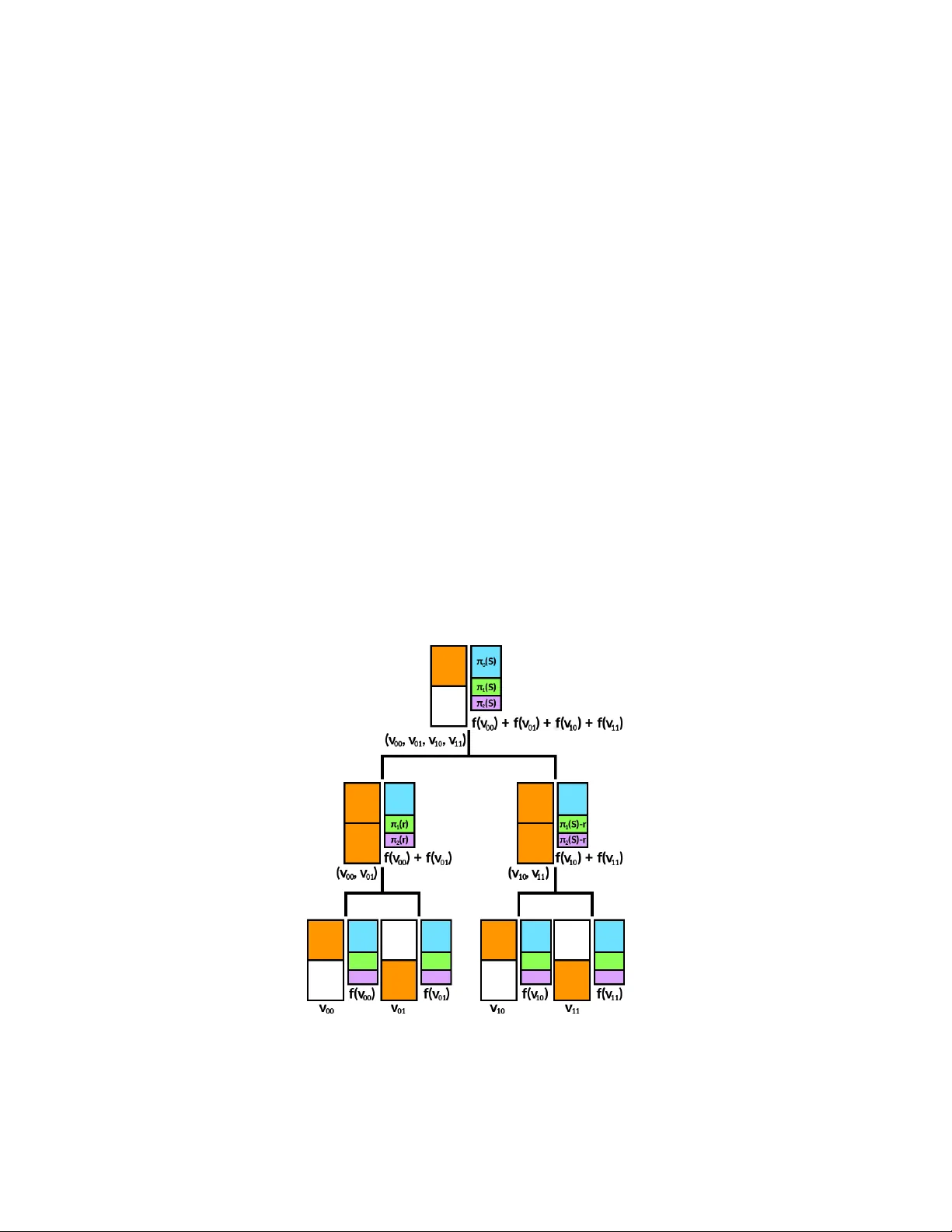
Quan tum Information Set Deco ding Algorithms Ghazal Kac higar 1 and Jean-Pierre Tillic h 2 1 Institut de Math ´ ematiques de Bordeaux Univ ersit´ e de Bordeaux T alence Cedex F-33405, F rance ghazal.kachigar@u-bordeaux.fr 2 Inria, E PI SECRET 2 rue Simone Iff, P aris 75012, F rance jean-pierre.tillich@inria.fr Abstract. The securit y of co de-based cryptosystems suc h as the McEliece cryptosystem relies primarily on the difficult y of decoding random linear codes. The b est decoding algo- rithms are all improv ements of an old algorithm due to Prange: they are known under the name of information set deco ding techniques. It is also important to assess the security of suc h cryptosystems against a quan tum computer. This research thread started in [22] and the best algorithm to date has b een Bernstein’s quan tising [5] of the simplest information set deco ding algorithm, namely Prange’s algorithm. It consists in applying Gro ver’s quan tum searc h to obtain a quadratic speed-up of Prange’s algorithm. In this paper, w e quan tise other information set deco ding algorithms by using quan tum walk techniques which were devised for the subset-sum problem in [6]. This results in improving the worst-case complexity of 2 0 . 06035 n of Bernstein’s algorithm to 2 0 . 05869 n with the b est algorithm presen ted here (where n is the co delength). Keyw ords: co de-based cryptograph y , quantum cryptanalysis, decoding algorithm. 1 In tro duction As humanit y’s technological prow ess improv es, quantum computers hav e mov ed from the realm of theoretical constructs to that of ob jects whose consequences for our other technologies, such as cryptograph y , must b e tak en into accoun t. Indeed, curren tly prev alen t public-key cryptosystems suc h as RSA and ECDH are vulnerable to Shor’s algorithm [26], whic h solv es factorisation and the discrete logarithm problem in polynomial time. Thus, in order to find a suitable replacement, it has b ecome necessary to study the impact of quan tum computers on other candidate cryptosystems. Co de-based cryptosystems suc h as the McEliece [20] and the Niederreiter [21] cryptosystems are suc h p ossible candidates. Their security essen tially relies on deco ding a linear co de. Recall that the deco ding problem consists, when giv en a linear code C and a noisy codeword c + e , in reco vering c , where c is an unkno wn co dew ord of C and e an unknown error of Hamming w eight w . A (binary) linear code C of dimension k and length n is sp ecified b y a full rank binary matrix H (i.e. a parity-c hec k matrix) of size ( n − k ) × n as C = { c ∈ F n 2 : H c T = 0 } . Since H ( c + e ) T = H c T + H e T = H e T the deco ding problem can b e rephrased as a syndome deco ding problem Pr oblem 1 (Syndr ome De c o ding Pr oblem). Giv en H and s T = H e T , where | e | = w , find e . This problem has been studied since the Sixties and despite significant efforts on this issue [23, 27, 11, 2, 18, 7, 4, 19] the b est algorithms for solving this problem [4, 19] are exp onen tial in the n umber of errors that hav e to b e corrected: correcting w errors in a binary linear code of length n and dimension k has with the aforementioned algorithms a cost of ˜ O (2 α ( k n , w n ) n ) where α ( R, ω ) is 2 Ghazal Kac higar and Jean-Pierre Tillich p ositiv e when R and ω are b oth positive. All these algorithms use in a crucial wa y the original idea due to Prange [23] and are kno wn under the name of Information Set Decoding (ISD) algorithms: they all tak e adv antage of the fact that there migh t exist a rather large set of positions con taining an information set of the co de 3 that is almost error free. All the efforts that hav e b een sp en t on this problem hav e only managed to decrease sligh tly this exp onent α ( R, ω ). The following table giv es an ov erview of the av erage time complexity of curren tly existing classical algorithms when w is the Gilbert-V arshamov distance d GV ( n, k ) of the co de. This quan tity is defined b y d GV ( n, k ) 4 = nH − 1 2  1 − k n  where H 2 is the binary entrop y function H 2 ( x ) 4 = − x log 2 ( x ) − (1 − x ) log 2 (1 − x ) and H − 1 2 its in verse defined from [0 , 1] to [0 , 1 2 ]. It corresp onds to the largest distance for whic h we ma y still expect a unique solution to the deco ding problem. If we wan t uniqueness of the solution, it can therefore b e considered as the hardest instance of deco ding. In the follo wing table, ω GV is defined b y the ratio ω GV 4 = d GV ( n, k ) /n . Author(s) Y ear max 0 ≤ R ≤ 1 α ( R, ω GV ) to 4 dec. places Prange [23] 1962 0.1207 Dumer [11] 1991 0.1164 MMT [18] 2011 0.1114 BJMM [4] 2012 0.1019 MO [19] 2015 0.0966 The question of using quantum algorithms to sp eed up ISD deco ding algorithms was first put forw ard in [22]. How ev er, the wa y Grov er’s algorithm was used in [22, Subsec. 3.5] to sp eed up deco ding did not allow for significant impro vemen ts ov er classical ISD algorithms. Later on, it w as sho wn b y Bernstein in [5] that it is p ossible to obtain m uch b etter speedups with Grov er’s algorithm: by using it for finding an error-free information set, the exp onen t of Prange’s algorithm can indeed b e halv ed. This pap er builds upon this wa y of using Grov er’s searc h algorithm, as well as the quan tum algorithms dev elopped by Bernstein, Jeffery , Lange and Meurer in [6] to solv e the subset sum prob- lem more efficien tly . The following table summarises the ingredients and av erage time complexit y of the algorithm of [5] and the new quantum algorithms presented in this pap er. Author(s) Y ear Ingredien ts max 0 ≤ R ≤ 1 α ( R, ω GV ) to 5 dec. places Bernstein [5] 2010 Prange+Gro ver 0.06035 This pap er 2017 Shamir-Sc hro epp el+Gro v er+QuantumW alk 0.05970 This pap er 2017 MMT+“1+1=0”+Grov er+Quan tumW alk 0.05869 A quic k calculation shows that the complexity exp onen t of our b est quantum algorithm, M M T QW , fulfils α MMTQW ≈ α Dumer 2 + 4 . 9 × 10 − 4 . Thus, our b est quantum algorithm impro ves in a small but non-trivial w ay on [5]. Several reasons will be giv en throughout this paper on why it has been difficult to do b etter than this. Notation. Throughout the pap er, we denote b y | e | the Hamming w eigh t of a v ector e . W e use the same notation for denoting the cardinalit y of a set, i.e. | S | denotes the cardinalit y of the set S . The meaning of this notation will b e clear from the context and we will use calligraphic letters to denote sets: S , I , M , . . . . W e use the standard O (), Ω (), Θ () notation and use the less standard ˜ O (), ˜ Ω (), ˜ Θ () notation to mean “ O (), Ω (), Θ (), when w e ignore logarithmic factors”. Here all the quantities we are in terested in are functions of the co delength n and we write f ( n ) = ˜ O ( g ( n )) for instance, when there exists a constan t k such suc h that f ( n ) = O  g ( n ) log k ( g ( n ))  . 3 An information set of a linear code C of dimension k is a set I of k positions such that when giv en { c i : i ∈ I } the co dew ord c of C is sp ecified entirely . Quan tum Information Set Decoding Algorithms 3 2 Quan tum search algorithms 2.1 Gro ver searc h Gro ver’s searc h algorithm [13, 14] is, along with its generalisation [8] whic h is used in this pap er, an optimal algorithm for solving the follo wing problem with a quadratic sp eed-up compared to the b est-possible classical algorithm. Pr oblem 2 (Unstructur e d se ar ch pr oblem). Given a set E and a function f : E → { 0 , 1 } , find an x ∈ E such that f ( x ) = 1. In other w ords, w e need to find an element that fulfils a certain prop ert y , and f is an oracle for deciding whether it do es. Moreov er, in the new results presented in this pap er, f will b e a quan tum algorithm. If we denote by ε the prop ortion of elements x of E such that f ( x ) = 1, Gro ver’s algorithm solves the problem ab o v e using O ( 1 √ ε ) queries to f , whereas in the classical setting this cannot b e done with less than O ( 1 ε ) queries. F urthermore, if the algorithm f executes in time T f on a verage, the a verage time complexit y of Gro ver’s algorithm will be O ( T f √ ε ). 2.2 Quan tum W alk Random W alk. Unstructured search problems as well as searc h problems with sligh tly more but still minimal structure ma y b e recast as graph search problems. Pr oblem 3 (Gr aph se ar ch pr oblem). Giv en a graph G = ( V , E ) and a set of v ertices M ⊂ V , called the set of marke d elements , find an x ∈ M . The graph search problem may then be solv ed using random walks (discrete-time Marko v chains) on the vertices of the graph. F rom now on, w e will take the graph to b e undirected, connected, and d -regular, i.e. suc h that each v ertex has exactly d neighbours. Markov chain. A Marko v c hain is given b y an initial probability distribution v and a stochastic transition matrix M . The transition matrix of a random walk on a graph (as sp ecified ab o ve) is obtained from the graph’s adjacency matrix A b y M = 1 d A . Eigenvalues and the sp e ctr al gap. A closer look at the eigen v alues and the eigenv ectors of M is needed in order to analyse the complexit y of a random w alk on a graph. The eigenv alues will be noted λ i and the corresp onding eigen v ectors v i . W e will admit the follo wing p oin ts (see [10]): (i) all the eigen v alues lie in the interv al [ − 1 , 1]; (ii) 1 is alw ays an eigen v alue, the corresponding eigenspace is of dimension 1; (iii) there is a corresp onding eigenv ector which is also a probability distribution (namely the uniform distribution u ov er the vertices). It is the unique stationary distribution of the random w alk. W e will supp ose that the eigenv alues are ordered from largest to smallest, so that λ 1 = 1 and v 1 = u . An imp ortan t v alue associated with the transition matrix of a Mark ov chain is its sp e ctr al gap , defined as δ 4 = 1 − max i =2 ,...,d | λ i | . Such a random walk on an undirected regular graph is alw ays r eversible and it is also irr e ducible because w e hav e assumed that the graph is connected. The random walk is ap erio dic in such a case if and only if the sp ectral gap δ is positive. In such a case, a long enough random w alk in the graph conv erges to the uniform distribution since for all η > 0, we ha v e || M k v − u || < η for k = ˜ O (1 /δ ), where v is the initial probability distribution. Finding a mark ed element b y running a Marko v c hain on the graph just consists in 4 Ghazal Kac higar and Jean-Pierre Tillich Algorithm 1: R andomW al k Input: G = ( E , V ), M ⊂ V , initial probabilit y distribution v Output: An element e ∈ M 1 Setup : Sample a vertex x according to v and initialise the data structure. 2 rep eat 3 Check : if curr ent vertex x is marke d then 4 return x 5 else 6 rep eat 7 Upda te : T ake one step of the random w alk and up date data structure accordingly . 8 un til x is sample d ac c or ding to a distribution close enough to the uniform distribution 9 Let T s b e the cost of Setup , T c b e the cost of Check and T u b e the cost of Upda te . It follo ws from the preceding considerations that ˜ O (1 /δ ) steps of the random walk are sufficient to sample x according to the uniform distribution. F urthermore, if w e note ε := | M | | V | the prop ortion of mark ed elemen ts, it is readily seen that the algorithm ends after O (1 /ε ) iterations of the outer lo op. Th us the complexit y of classical random walk is T s + 1 ε  T c + 1 δ T u  . Sev eral quantum v ersions of random walk algorithms hav e been prop osed by many authors, notably Ambainis [1], Szegedy [28], and Magniez, Nay ak, Roland and San tha [17]. A survey of these results can b e found in [24]. W e use here the follo wing result Theorem 1 ([17]). L et M b e an ap erio dic, irr e ducible and r eversible Markov chain on a gr aph with sp e ctr al gap δ , and ε := | M | | V | as ab ove. Then ther e is a quantum walk algorithm that finds an element in M with c ost T s + 1 √ ε  T c + 1 √ δ T u  (1) Johnson graphs and product graphs. With the exception of Gro ver’s searc h algorithm seen as a quantum w alk algorithm, to date an o v erwhelming ma jority of quantum walk algorithms are based on Johnson graphs or a v ariant thereof. The deco ding algorithms which shall b e presented in this pap er rely on cartesian products of Johnson graphs. All of these ob jects are defined in this section and some imp ortan t prop erties are men tioned. Definition 1 (Johnson graphs). A Johnson gr aph J ( n, r ) is an undir e cte d gr aph whose vertic es ar e the subsets c ontaining r elements of a set of size n , with an e dge b etwe en two vertic es S and S 0 iff | S ∩ S 0 | = r − 1 . In other wor ds, S is adjac ent to S 0 if S 0 c an b e obtaine d fr om S by r emoving an element and adding a new element in its plac e. It is clear that J ( n, r ) has  n r  v ertices and is r ( n − r )-regular. Its sp ectral gap is giv en by δ = n r ( n − r ) . (2) Definition 2 (Cartesian pro duct of graphs). L et G 1 = ( V 1 , E 1 ) and G 2 = ( V 2 , E 2 ) b e two gr aphs. Their c artesian pr o duct G 1 × G 2 is the gr aph G = ( V , E ) wher e: 1. V = V 1 × V 2 , i.e. V = { v 1 v 2 | v 1 ∈ V 1 , v 2 ∈ V 2 } 2. E = { ( u 1 u 2 , v 1 v 2 ) | ( u 1 = v 1 ∧ ( u 2 , v 2 ) ∈ E 2 ) ∨ (( u 1 , v 1 ) ∈ E 1 ∧ u 2 = v 2 ) } The sp ectral gap of products of Johnson graphs is given b y Theorem 2 (Cartesian pro duct of Johnson graphs). L et J ( n, r ) = ( V , E ) , m ∈ N and J m ( n, r ) := × m i =1 J ( n, r ) = ( V m , E m ) . Then: 1. J m ( n, r ) has  n r  m vertic es and is md -r e gular wher e d = r ( n − r ) . Quan tum Information Set Decoding Algorithms 5 2. We wil l write δ ( J ) r esp. δ ( J m ) for the sp e ctr al gaps of J ( n, r ) r esp. J m ( n, r ) . Then: δ ( J m ) ≥ 1 m δ ( J ) . 3. The r andom walk asso ciate d with J m ( n, r ) is ap erio dic, irr e ducible and r eversible for al l p ositive m , n and r < n . F or a proof of this statement, see the appendix. 3 Generalities on classical and quan tum deco ding W e first recall how the simplest ISD algorithm [23] and its quan tised version [5] work and then giv e a skeleton of the structure of more sophisticated classical and quan tum versions. 3.1 Prange’s algorithm and Bernstein’s algorithm Recall that the goal is to find e of w eight w giv en s T = H e T , where H is an ( n − k ) × n matrix. In other w ords, the problem w e aim to solv e is finding a solution to an underdetermined linear system of n − k equations in n v ariables and the solution is unique owing to the weigh t condition. Prange’s algorithm is based on the follo wing observ ation: if it is known that k giv en components of the error vector are zero, the error positions are among the n − k remaining comp onen ts. In other w ords, if we kno w for sure that the k corresponding v ariables are not inv olv ed in the linear system, then the error vector can be found b y solving the resulting linear system of n − k equations in n − k v ariables in polynomial time. The hard part is finding a correct size- k set (of indices of the comp onen ts). Prange’s algorithm samples suc h sets and solv es the resulting linear equation un til an error v ector of weigh t w is found. The probability for finding such a set is of order Ω  ( n − k w ) ( n w )  and therefore Prange’s algorithm has complexit y O  n w   n − k w  ! = ˜ O  2 α Prange ( R,ω ) n  where α Prange ( R, ω ) = H 2 ( ω ) − (1 − R ) H 2  ω 1 − R  b y using the well kno wn formula for binomials  n w  = ˜ Θ  2 H 2 ( w n ) n  . Bernstein’s algorithm consists in using Gro ver’s algorithm to find a correct size- k set. Indeed, an oracle for chec king that a size- k set is correct can b e obtained by following the same steps as in Prange’s algorithm, i.e. deriving and solving a linear system of n − k equations in n − k v ariables and returning 1 iff the resulting error vector has weigh t w . Th us the complexity of Bernstein’s algorithm is the square ro ot of that of Prange’s algorithm, i.e. α Bernstein = α Prange 2 . 3.2 Generalised ISD algorithms More sophisticated classical ISD algorithms [27, 11, 12, 7, 18, 4, 19] generalise Prange’s algorithm in the follo wing w ay: they introduce a new parameter p and allow p error positions inside of th e size- k set (henceforth denoted by S ). F urthermore, from Dumer’s algorithm on wards, a new parameter ` is introduced and the set S is taken to be of size k + ` . This even t happ ens with probability P `,p 4 = ( k + ` p )( n − k − ` w − p ) ( n w ) . The p oin t is that Prop osition 1. Assume that the r estriction of H to the c olumns b elonging to the c omplement of S is a matrix of ful l r ank, then 6 Ghazal Kac higar and Jean-Pierre Tillich (i) the r estriction e 0 of the err or to S is a solution to the syndr ome de c o ding pr oblem H 0 e 0 T = s 0 T . (3) with H 0 b eing an ` × ( k + ` ) binary matrix, | e 0 | = p and H 0 , s 0 that c an b e c ompute d in p oly- nomial time fr om S , H and s ; (ii) onc e we have such an e 0 , ther e is a unique e whose r estriction to S is e qual to e 0 and which satisfies H e T = s T . Such an e c an b e c ompute d fr om e 0 in p olynomial time. R emark: The condition in this prop osition is met with very large probability when H is c hosen uniformly at random: it fails to hold with probabilit y which is only O (2 − ` ). Pr o of. Without loss of generalit y assume that S is giv en b y the k + ` first positions. By p erforming Gaussian elimination, w e lo ok for a square matrix U such that U H =  H 0 0 ` H ” I n − k − `  That such a matrix exists is a consequence of the fact that H restricted to the last n − k − ` p ositions is of full rank. W rite now e = ( e 0 , e ”) where e 0 is the word formed by the k + ` first en tries of e . Then U s T = U H e T = H 0 e 0 T H ” e 0 T + e ” T ! . If w e write U s T as ( s 0 , s ”) T , where s 0 T is the v ector formed by the ` first en tries of U s T , then w e reco ver e from e 0 b y using the fact that H ” e 0 T + e ” T = s ” T . u t F rom now on, w e denote by Σ and h the functions that can be computed in polynomial time that are promised b y this prop osition, i.e. s 0 = Σ ( s, H , S ) e = h ( e 0 ) In other words, all these algorithms solve in a first step a new instance of the syndrome deco ding problem with different parameters. The difference with the original problem is that if ` is small, whic h is the case in general, there is not a single solution anymore. Ho wev er searching for all (or a large set of them) can b e done more efficiently than just brute-forcing ov er all errors of w eigh t p on the set S . Once a p ossible solution e 0 to (3) is found, e is recov ered as explained before. The main idea which a v oids brute forcing ov er all p ossible errors of w eight p on S is to obtain candidates e 0 b y solving an instance of a generalised k -sum problem that we define as follo ws. Pr oblem 4 (gener alise d k -sum pr oblem). Consider an Ab elian group G , an arbitrary set E , a map f from E to G , k subsets V 0 , V 1 , . . . , V k − 1 of E , another map g from E k to { 0 , 1 } , and an elemen t S ∈ G . Find a solution ( v 0 , . . . , v k − 1 ) ∈ V 0 × . . . V k − 1 suc h that we ha ve at the same time (i) f ( v 0 ) + f ( v 1 ) · · · + f ( v k − 1 ) = S (subset-sum condition); (ii) g ( v 0 , . . . , v k − 1 ) = 0 (( v 0 , . . . , v k − 1 ) is a ro ot of g ). Dumer’s ISD algorithm, for instance, solv es the 2-sum problem in the case where G = F ` 2 , E = F k + ` 2 , f ( v ) = H 0 v T V 0 = { ( e 0 , 0 ( k + ` ) / 2 ) ∈ F k + ` 2 : e 0 ∈ F ( k + ` ) / 2 2 , | e 0 | = p/ 2 } V 1 = { (0 ( k + ` ) / 2 , e 1 ) ∈ F k + ` 2 : e 1 ∈ F ( k + ` ) / 2 2 , | e 1 | = p/ 2 } and g ( v 0 , v 1 ) = 0 if and only if e = h ( e 0 ) is of w eigh t w where e 0 = v 0 + v 1 . A solution to the 2-sum problem is then clearly a solution to the deco ding problem b y construction. The p oin t is that the Quan tum Information Set Decoding Algorithms 7 2-sum problem can b e solved in time which is muc h less than | V 0 | · | V 1 | . F or instance, this can clearly b e ac hiev ed in exp ected time | V 0 | + | V 1 | + | V 0 |·| V 1 | | G | and space | G | b y storing the elements v 0 of V 0 in a hashtable at the address f ( v 0 ) and then going ov er all elements v 1 of the other set to c heck whether or not the address S − f ( v 1 ) con tains an element. The term | V 0 |·| V 1 | | G | accoun ts for the exp ected n um b er of solutions of the 2-sum problem when the elements of V 0 and V 1 are c hosen uniformly at random in E (which is the assumption what w e are going to make from on). This is precisely what Dumer’s algorithm does. Generally , the size of G is c hosen suc h that | G | = Θ ( | V i | ) and the space and time complexit y are also of this order. Generalised ISD algorithms are th us composed of a lo op in whic h first a set S is sampled and then an error vector having a certain form, namely with p error positions in S and w − p error p ositions outside of S , is sough t. Th us, for eac h ISD algorithm A , w e will denote by S ear ch A the algorithm whose exact implemen tation dep ends on A but whose sp ecification is alw ays S ear ch A : S , H , s, w, p → { e | e has weigh t p on S and w eight w − p on S and s T = H e T } ∪ { N U LL } , where S is a set of indices, H is the parity-c hec k matrix of the code and s is the syndrome of the error we are lo oking for. The following pseudo-co de gives the structure of a generalised ISD algorithm. Algorithm 2: ISD Sk eleton Input: H , s , w , p Output: e of weigh t w suc h that s T = H e T 1 rep eat 2 Sample a set of indices S ⊂ { 1 , ..., n } 3 e ← S earch A ( S , H , s, w , p ) 4 un til | e | = w 5 return e Th us, if we note P A the probabilit y , dep enden t on the algorithm A , that the sampled set S is correct and that A finds e 4 , and T A the execution time of the algorithm S ear ch A , the complexity of generalised ISD algorithms is O  T A P A  . T o construct generalised quan tum ISD algorithms, we use Bernstein’s idea of using Gro v er search to look for a correct set S . How ev er, now eac h query made b y Gro ver searc h will take time which is essentially the time complexity of S earch A . Consequen tly , the complexit y of generalised quantum ISD algorithms is giv en by the follo wing form ula: O  T A √ P A  = O   s T 2 A P A   . (4) An immediate consequence of this form ula is that, in order to halve the complexity exp onen t of a giv en classical algorithm, we need a quantum algorithm whose searc h subroutine is “t wice” as efficien t. 4 Solving the generalised 4-sum problem with quantum w alks and Gro v er searc h 4.1 The Shamir-Sc hro epp el idea As explained in Section 3, the more sophisticated ISD algorithms solve during the inner step an instance of the generalised k -sum problem. The issue is to get a goo d quantum version of the classical algorithms used to solv e this problem. That this task is non trivial can already be guessed from Dumer’s algorithm. Recall that it solves the generalised 2-sum problem in time and space complexit y O ( V ) when V = | V 0 | = | V 1 | = Θ ( | G | ). The problem is that if w e wan ted a quadratic 4 In the case of Dumer’s algorithm, for instance, ev en if the restriction of e to S is of weigh t p , Dumer’s algorithm may fail to find it since it do es not split ev enly on b oth sides of the bipartition of S . 8 Ghazal Kac higar and Jean-Pierre Tillich sp eedup when compared to the classical Dumer algorithm, then this would require a quantum algorithm solving the same problem in time O  V 1 / 2  , but this seems problematic since naive w ays of quan tising this algorithm stumble on the problem that the space complexity is a low er b ound on the time complexit y of the quantum algorithm. This strongly motiv ates the c hoice of w ays of solving the 2-sum problem b y using less memory . This can b e done through the idea of Shamir and Sc hro eppel [25]. Note that the v ery same idea is also used for the same reason to speed up quantum algorithms for the subset sum problem in [6, Sec. 4]. T o explain the idea, supp ose that G factorises as G = G 0 × G 1 where | G 0 | = Θ ( | G 1 | ) = Θ ( | G | 1 / 2 ). Denote for i ∈ { 0 , 1 } by π i the pro jection from G onto G i whic h to g = ( g 0 , g 1 ) asso ciates g i . The idea is to construct f ( V 0 ) and f ( V 1 ) themselv es as f ( V 0 ) = f ( V 00 ) + f ( V 01 ) and f ( V 1 ) = f ( V 10 ) + f ( V 11 ) in such a wa y that the V ij ’s are of size O ( V 1 / 2 ) and to solv e a 4-sum problem b y solving v arious 2-sum problems. In our co ding theoretic setting, it will b e more con venien t to explain ev erything directly in terms of the 4-sum problem which is giv en in this case by Pr oblem 5. Assume that k + ` and p are multiples of 4. Let G = F ` 2 , E = F k + ` 2 , f ( v ) = H 0 v T V 00 4 = { ( e 00 , 0 3( k + ` ) / 4 ) ∈ F k + ` 2 : e 00 ∈ F ( k + ` ) / 4 2 , | e 00 | = p/ 4 } V 01 4 = { (0 ( k + ` ) / 4 , e 01 , 0 ( k + ` ) / 2 ) ∈ F k + ` 2 : e 01 ∈ F ( k + ` ) / 4 2 , | e 01 | = p/ 4 } V 10 4 = { (0 ( k + ` ) / 2 , e 10 , 0 ( k + ` ) / 4 ) ∈ F k + ` 2 : e 10 ∈ F ( k + ` ) / 4 2 , | e 10 | = p/ 4 } V 11 4 = { (0 3( k + ` ) / 4 , e 11 ) ∈ F k + ` 2 : e 11 ∈ F ( k + ` ) / 4 2 , | e 11 | = p/ 4 } and S b e some element in G . Find ( v 00 , v 01 , v 10 , v 11 ) in V 00 × V 01 × V 10 × V 11 suc h that f ( v 00 ) + f ( v 01 ) + f ( v 10 ) + f ( v 11 ) = S and h ( v 00 + v 01 + v 10 + v 11 ) is of w eight w . Let us explain now how the Shamir-Schroepp el idea allows us to solve the 4-sum problem in time O ( V ) and space O  V 1 / 2  when the V ij ’s are of order O  V 1 / 2  , | G | is of order V and when G decomp oses as the product of tw o groups G 0 and G 1 b oth of size Θ  V 1 / 2  . The basic idea is to solv e for all p ossible r ∈ G 1 the follo wing 2-sum problems π 1 ( f ( v 00 )) + π 1 ( f ( v 01 )) = r (5) π 1 ( f ( v 10 )) + π 1 ( f ( v 11 )) = π 1 ( S ) − r (6) Once these problems are solved we are left with O  V 1 / 2 V 1 / 2 /V 1 / 2  = O  V 1 / 2  solutions to the first problem and O  V 1 / 2  solutions to the second. T aking any pair ( v 00 , v 01 ) solution to (5) and ( v 10 , v 11 ) solution to (6) yields a 4-tuple whic h is a partial solution to the 4-sum problem π 1 ( f ( v 00 )) + π 1 ( f ( v 01 )) + π 1 ( f ( v 10 )) + π 1 ( f ( v 11 )) = r + π 1 ( S ) − r = π 1 ( S ) . Let V 0 0 b e the set of all pairs ( v 00 , v 01 ) w e hav e found for the first 2-sum problem (5), whereas V 0 1 is the set of all solutions to (6). T o ensure that f ( v 00 ) + f ( v 01 ) + f ( v 10 ) + f ( v 11 ) = S w e just hav e to solv e the following 2-sum problem π 0 ( f ( v 00 )) + π 0 ( f ( v 01 )) | {z } f 0 ( v 00 ,v 01 ) + π 0 ( f ( v 10 )) + π 0 ( f ( v 11 )) | {z } f 0 ( v 10 ,v 11 ) = π 0 ( S ) and g ( v 00 , v 01 , v 10 , v 11 ) = 0 where ( v 00 , v 01 ) is in V 0 0 , ( v 10 , v 11 ) is in V 0 1 and g is the function whose ro ot we w ant to find for the original 4-sum problem. This is again of complexity O  V 1 / 2 V 1 / 2 /V 1 / 2  = O  V 1 / 2  . Checking a particular v alue of r tak es therefore O  V 1 / 2  op erations. Since we hav e Θ  V 1 / 2  v alues to chec k, the total complexity is O  V 1 / 2 V 1 / 2  = O ( V ), that is the same as b efore, but we need only O  V 1 / 2  memory to store all in termediate sets. Quan tum Information Set Decoding Algorithms 9 Fig. 1. The Shamir-Schroepp el idea in the deco ding context (see Problem 5): the supp ort of the elements of V ij is repre sented in orange, while the blue and green colours represent G 0 resp. G 1 . 4.2 A quan tum version of the Shamir-Sc hro epp el algorithm By follo wing the approach of [6], we will define a quan tum algorithm for solving the 4-sum problem b y combining Gro ver searc h with a quan tum walk with a complexit y given b y Prop osition 2. Consider the gener alise d 4 -sum pr oblem with sets V u of size V . Assume that G c an b e de c omp ose d as G = G 0 × G 1 . Ther e is a quantum algorithm for solving the 4 -sum pr oblem running in time ˜ O  | G 1 | 1 / 2 V 4 / 5  as so on as | G 1 | = Ω  V 4 / 5  and | G | = Ω  V 8 / 5  . This is nothing but the idea of the algorithm [6, Sec. 4] laid out in a more general context. The idea is as in the classical algorithm to lo ok for the righ t v alue r ∈ G 1 . This can be done with Gro ver searc h in time O  | G 1 | 1 / 2  instead of O ( | G 1 | ) in the classical case. The quantum w alk is then used to solv e the following problem: Pr oblem 6. Find ( v 00 , v 01 , v 10 , v 11 ) in V 00 × V 01 × V 10 × V 11 suc h that π 1 ( f ( v 00 )) + π 1 ( f ( v 01 )) = r π 1 ( f ( v 10 )) + π 1 ( f ( v 11 )) = π 1 ( S ) − r π 0 ( f ( v 00 )) + π 0 ( f ( v 01 )) + π 0 ( f ( v 10 )) + π 0 ( f ( v 11 )) = π 0 ( S ) g ( v 00 , v 01 , v 10 , v 11 ) = 0 . F or this, we choose subsets U i ’s of the V i ’s of a same size U = Θ  V 4 / 5  and run a quantum w alk on the graph whose v ertices are all possible 4-tuples of sets of this kind and tw o 4-tuples ( U 00 , U 01 , U 10 , U 11 ) and ( U 0 00 , U 0 01 , U 0 10 , U 0 11 ) are adjacen t if and only if we ha ve for all i ’s but one U 0 i = U i and for the remaining U 0 i and U i w e hav e | U 0 i ∩ U i | = U − 1. Notice that this graph is nothing but J 4 ( V , U ). By following [6, Sec. 4] it can be prov ed that 10 Ghazal Kac higar and Jean-Pierre Tillich Prop osition 3. Under the assumptions that | G 1 | = Ω  V 4 / 5  and | G | = Ω  V 8 / 5  , it is p ossible to set up a data structur e of size O ( U ) to implement this quantum walk such that (i) setting up the data structur e takes time O ( U ) ; (ii) che cking whether a new 4 -tuple le ads to a solution to the pr oblem ab ove (and outputting the solution in this c ase) takes time O (1) , (iii) up dating the data structur e takes time O (log U ) . The pro of whic h w e give is adapted from [6, Sec. 4]. Pr o of. 1. Setting up the data structure takes time O ( U ) . The data structure is set up more or less in the same wa y as in classical Shamir-Schroepp el’s algorithm, i.e. b y solving tw o 2-sum problems first and then using the result to solv e a third and last 2-sum problem. There are ho wev er the following differences: (i) W e no longer keep the results in a hash table but in some other type of ordered data structure whic h allows for the insertion, deletion and searc h op erations to be done in O (log U ) time. F or instance, [6] c hose radix trees. More detail will be given when w e look at the Upd a te op eration. (ii) Because w e no longer use hashtables, we will need t wo data structures at eac h step, one to k eep trac k of f ( v 00 ) along with the associated v 00 , f ( v 00 ) + f ( v 01 ) along with the associated ( v 00 , v 01 ), etc. and another to k eep track of v 00 , ( v 00 , v 01 ), etc. separately . If w e denote the first family of data structures b y D f and the second family by D V , this giv es a total of 13 data structures (7 of t yp e D V and 6 of t yp e D f , because no data structure is needed to store the sum of all four v ectors which is simply S ). Solving the first tw o 2-sum problems tak es time | U i 0 | + | U i 1 | + | U i 0 | . | U i 1 | | G 1 | , i = 0 , 1, which is O ( U ) b ecause | G 1 | = Ω  V 4 / 5  = Ω ( U ). Denote b y U 0 resp. U 1 the set of solutions to these t wo problems. These solutions are used to solv e the second 2-sum, problem, which tak es time | U 0 | + | U 1 | + | U 0 | . | U 1 | | G 0 | = O ( U ) due to G 0 = G / G 1 and | G | = Ω  V 8 / 5  . Th us, setting up the data structure takes time O ( U ). 2. Up dating the data structure tak es time O (log U ) . Recall that the data structures are c hosen such that the insertion, deletion and search opera- tions tak e O (log U ) time, and also that there are t wo data structures p ertaining to eac h v ector or pair of v ectors, for a total of 13 data structures. Recall also that the up date step consists in moving from one vertex of the Johnson graph J 4 ( V , U ) to one that is adjacen t to it. Suppose, without loss of generalit y , that w e mov e from the vertex ( U 00 , U 01 , U 10 , U 11 ) to ( U 0 00 , U 01 , U 10 , U 11 ). Thus, a v 00 ∈ U 00 has b een replaced b y a u 00 ∈ U 00 . Then, the low cost of the up date step relies up on the follo wing fundamental insigh t: there are in all U possible w a ys of writing the sum π 1 ( f ( u 00 )) + π 1 ( f ( v 01 )) (one for eac h v 01 ∈ U 01 ). But we hav e one further constrain t whic h is that this sum needs to b e equal to a given r ∈ G 1 . Th us, there are on av erage | U ij | | G 1 | = O (1) v alues of v 01 ∈ U 01 whic h give a solution. Note that the same argumen t applies for the num b er of ( v 10 , v 11 ) ∈ U 1 that fulfil the condition π 0 ( f ( u 00 )) + π 0 ( f ( v 01 )) + π 0 ( f ( v 10 )) + π 0 ( f ( v 11 )) = π 0 ( S ) for a giv en ( u 00 , v 01 ) ∈ U 0 (where π 0 ( S ) ∈ G 0 ), for in this case there are on a verage | U 0 | | G 0 | = O (1) suc h elements. Quan tum Information Set Decoding Algorithms 11 This allows us to pro ceed as follo ws: we imp ose a constan t limit on the n umber of v 01 ∈ U 01 that correspond to a given u 00 ∈ U 00 at eac h up date operation. A similar limit is imp osed on the n umber of ( v 10 , v 11 ) ∈ U 1 . The probabilit y of reaching this limit is negligeable, and if it is reac hed, w e re-initialise the data structure, so this do es not modify the o verall complexity of the algorithm. Note also that there is no problem when the opp osite situation happ ens, i.e. when there are no v 01 ∈ U 01 corresp onding to a given u 00 ∈ U 00 . Indeed, while this ma y result in the data structure b eing depleted, this is a temp orary situation and the data structure will b e refilled o v er time as more suitable elements occur. W e now enumerate the steps needed to up date the data structure. What we need to do is to remov e the old elemen t v 00 and everything that has b een constructed using it, and add u 00 and ev erything that it allows to construct (within the limits discussed ab o ve). First, to remo ve v 00 and the other elemen ts it affects, we need to do the follo wing: (a) Find and delete v 00 from the data structure D U 00 . (b) Calculate f ( v 00 ), then find and delete it from the data structure D f 00 . (c) Find at most a constan t num b er of ( v 00 , v 01 ) in D U 0 and remo ve them. (d) F or eac h of these ( v 00 , v 01 ), calculate f ( v 00 ) + f ( v 01 ) and remo ve it from D f 0 . (e) Find at most a constan t num b er of ( v 00 , v 01 , v 01 , v 11 ) in D U and remo ve them. This step uses operations of negligeable cost (calculating f ( v 00 ), etc.) and the num ber of op- erations of cost log( U ) whic h it uses is b ounded by a constant. Thus it takes time O (log( U )). T o add u 00 and other new elemen ts dep ending on it, w e pro ceed as follows: (a) Insert u 00 in D U 00 . (b) Calculate f ( u 00 ), then insert it in D f 00 . (c) Calculate x = r − π 1 ( f ( u 00 )) and find if there are elements y in D f 01 suc h that π 1 ( y ) = x . F or a constant n umber of asso ciated v 01 , insert ( u 00 , v 01 ) in D U 0 and in D f 0 asso ciated with r . (d) Similarly there are a constant num b er of ( v 01 , v 11 ) that need to b e up dated, for those calculate g ( u 00 , v 01 , v 10 , v 11 ). If it is equal to zero, insert ( v 00 , v 01 , v 10 , v 11 ) in D U . It is easy to see that this step also takes time O (log( U )). 3. Chec king whether a new 4 -tuple leads to a solution of the problem takes time O (1) . Chec king that the righ t 4-tuple is in D U requires looking for it in D U at the first step of the algorithm. This costs O ( √ U ) using Grov er search. A t the follo wing steps of the algorithm, it is enough to c hec k the new elemen ts (whose n um b er is b ounded by a constant) that hav e b een added to D U . So the c hecking cost is O (1) ov erall. u t Prop osition 2 is essen tially a corollary of this prop osition. Pr o of (Pr o of of Pr op osition 2). Recall that the cost of the quan tum walk is given by T s + 1 √ ε  T c + 1 √ δ T u  where T s , T c , T u , ε and δ are the setup cost, the chec k cost, the update cost, the prop ortion of mark ed elemen ts and the sp ectral gap of the quan tum w alk. F rom Proposition 3, w e kno w that T s = O ( U ) = O  V 4 / 5  , T c = O (1), and T u = O (log U ). Recall that the sp ectral gap of J ( V , U ) is equal to V U ( V − U ) b y (2). This quantit y is larger than 1 U and by using Theorem 2 on the cartesian pro duct of Johnson graphs, w e obtain δ = Θ  1 U  . No w for the prop ortion of marked elemen ts we argue as follo ws. If Problem 6 has a solution ( v 00 , v 01 , v 10 , v 11 ), then the probability that each of the sets U i con tains v i is precisely U /V = Θ  V − 1 / 5  . The probability ε that all the U i ’s contain v i is then Θ  V − 4 / 5  . This gives a total cost of O  V 4 / 5  + O  V 2 / 5   O (1) + O  V 2 / 5  O (log U )  = ˜ O  V 4 / 5  . When w e multiply this b y the cost of Gro ver’s algorithm for finding the right r we hav e the aforemen tioned complexity . u t 12 Ghazal Kac higar and Jean-Pierre Tillich 4.3 Application to the deco ding problem When applying this approac h to the deco ding problem w e obtain Theorem 3. We c an de c o de w = ωn err ors in a r andom line ar c o de of length n and r ate R = k n with a quantum c omplexity of or der ˜ O  2 α SSQW ( R,ω ) n  wher e α SSQW ( R, ω ) 4 = min ( π ,λ ) ∈ R   H 2 ( ω ) − (1 − R − λ ) H 2  ω − π 1 − R − λ  − 2 5 ( R + λ ) H 2  π R + λ  2   R 4 =  ( π , λ ) ∈ [0 , ω ] × [0 , 1) : λ = 2 5 ( R + λ ) H 2  π R + λ  , π ≤ R + λ, λ ≤ 1 − R − ω + π  Pr o of. Recall (see (4)) that the quantum complexit y is given b y ˜ O T SSQW p P SSQW ! (7) where T SSQW is the complexity of the combination of Grov er’s algorithm and quan tum walk solving the generalised 4-sum problem sp ecified in Problem 6 and P SSQW is the probability that the random set of k + ` positions S and its random partition in 4 sets of the same size that are c hosen is suc h that all four of them contain exactly p/ 4 errors. Note that p and ` are c hosen suc h that k + ` and p are divisible b y 4. P SSQW is giv en by P SSQW =  k + ` 4 p 4  4  n − k − ` w − p   n w  Therefore ( P SSQW ) − 1 / 2 = ˜ O 2 H 2 ( ω ) − (1 − R − λ ) H 2 ( ω − π 1 − R − λ ) − ( R + λ ) H 2 ( π R + λ ) 2 n ! (8) where λ 4 = ` n and π 4 = p n . T SSQW is giv en by Proposition 2: T SSQW = ˜ O  | G 1 | 1 / 2 V 4 / 5  where the sets in volv ed in the generalised 4-sum problem are sp ecified in Problem 6. This giv es V =  k + ` 4 p 4  W e c ho ose G 1 as G 1 = F d ` 2 e 2 (9) and the assumptions of Prop osition 2 are v erified as so on as 2 ` = Ω  V 8 / 5  . whic h amounts to 2 ` = Ω  k + ` 4 p 4  8 / 5 ! This explains the condition λ = 2 5 ( R + λ ) H 2  π R + λ  (10) Quan tum Information Set Decoding Algorithms 13 found in the definition of the region R . With the choices (9) and (10), w e obtain T SSQW = ˜ O  V 6 / 5  = ˜ O  2 3 10 ( R + λ ) H 2 ( π R + λ ) n  (11) Substituting for P SSQW and T SSQW the expressions given by (8) and (11) finishes the proof of the theorem. u t 5 Impro v ements obtained b y the represen tation technique and “1 + 1 = 0” There are tw o techniques that can b e used to sp eed up the quantum algorithm of the previous section. The r epr esentation te chnique. It was in troduced in [15] to sp eed up algorithms for the subset- sum algorithm and used later on in [18] to improv e deco ding algorithms. The basic idea of the represen tation technique in the context of the subset-sum or deco ding algorithms consists in (i) c hanging slightly the underlying (generalised) k -sum problem which is solv ed by in tro ducing sets V i for which there are (exponentially) many solutions to the problem P i f ( v i ) = S b y using redundan t represen tations, (ii) noticing that this allo ws us to put additional subset-sum conditions on the solution. In the decoding context, instead of considering sets of errors with non-o verlapping support, the idea that allo ws us to obtain man y different represen tations of a same solution is just to consider sets V i corresp onding to errors with o v erlapping supp orts. In our case, w e could ha v e tak en instead of the four sets defined in the previous section the following sets V 00 = V 10 4 = { ( e 00 , 0 ( k + ` ) / 2 ) ∈ F k + ` 2 : e 00 ∈ F ( k + ` ) / 2 2 , | e 00 | = p/ 4 } V 01 = V 11 4 = { (0 ( k + ` ) / 2 , e 01 ) ∈ F k + ` 2 : e 01 ∈ F ( k + ` ) / 2 2 , | e 01 | = p/ 4 } Clearly a v ector e of weigh t p can b e written in many different wa ys as a sum v 00 + v 01 + v 10 + v 11 where v ij b elongs to V ij . This is (essentially) due to the fact that a vector of weigh t p can b e written in  p p/ 2  = ˜ O (2 p ) w ays as a sum of t wo v ectors of w eight p/ 2. The p oint is that if we apply no w the same algorithm as in the previous section and lo ok for solutions to Problem 5, there is not a single v alue of r that leads to the righ t solution. Here, ab out 2 p v alues of r will do the same job. The sp eedup obtained by the represen tation tec hnique is a consequence of this phenomenon. W e can ev en impro ve on this representation tec hnique b y using the 1 + 1 = 0 phenomenon as in [4]. The “ 1 + 1 = 0 ” phenomenon. Instead of c ho osing the V i ’s as explained ab ov e we will actually c ho ose the V i ’s as V 00 = V 10 4 = { ( e 00 , 0 ( k + ` ) / 2 ) ∈ F k + ` 2 : e 00 ∈ F ( k + ` ) / 2 2 , | e 00 | = p 4 + ∆p 2 } (12) V 01 = V 11 4 = { (0 ( k + ` ) / 2 , e 01 ) ∈ F k + ` 2 : e 01 ∈ F ( k + ` ) / 2 2 , | e 01 | = p 4 + ∆p 2 } (13) A vector e of w eigh t p in F k + ` 2 can indeed by represen ted in many wa ys as a sum of 2 vectors of w eight p 2 + ∆p . More precisely , suc h a v ector can be represented in  p p/ 2  k + ` − p ∆p  w ays. Notice that this num b er of representations is greater than the n umber 2 p that we had before. This explains wh y choosing an appropriate p ositiv e v alue ∆p allows us to impro v e on the previous choice. The quan tum algorithm for decoding follows the same pattern as in the previous section: (i) w e lo ok with Gro ver’s searc h algorithm for a righ t set S of k + ` p ositions suc h that the restriction e 0 of the error e we lo ok for is of weigh t p on this subset and then (ii) we searc h for e 0 b y solving a generalised 4-sum problem with a com bination of Gro v er’s algorithm and a quantum w alk. W e will use for the second point the following prop osition whic h quan tifies ho w muc h w e gain when there are m ultiple representations/solutions: 14 Ghazal Kac higar and Jean-Pierre Tillich Prop osition 4. Consider the gener alise d 4 -sum pr oblem with sets V u of size O ( V ) . Assume that G c an b e de c omp ose d as G = G 0 × G 1 × G 2 . F urthermor e assume that ther e ar e Ω ( | G 2 | ) solutions to the 4 -sum pr oblem and that we c an fix arbitr arily the value π 2 ( f ( v 00 ) + f ( v 01 )) of a solution to the 4 -sum pr oblem, wher e π 2 is the mapping fr om G = G 0 × G 1 × G 2 to G 2 which maps ( g 0 , g 1 , g 2 ) to g 2 . Ther e is a quantum algorithm for solving the 4 -sum pr oblem running in time ˜ O  | G 1 | 1 / 2 V 4 / 5  as so on as | G 1 | · | G 2 | = Ω  V 4 / 5  and | G | = Ω  V 8 / 5  . Pr o of. Let us first in tro duce a few notations. W e denote by π 12 the “pro jection” from G = G 0 × G 1 × G 2 to G 1 × G 2 whic h asso ciates to ( g 0 , g 1 , g 2 ) the pair ( g 1 , g 2 ) and by π 0 the pro jection from G to G 0 whic h maps ( g 0 , g 1 , g 2 ) to g 0 . As in the previous section, we solv e with a quantum w alk the follo wing problem: w e fix an elemen t r = ( r 1 , r 2 ) in G 1 × G 2 and find (if it exists) ( v 00 , v 01 , v 10 , v 11 ) in V 00 × V 01 × V 10 × V 11 suc h that π 12 ( f ( v 00 )) + π 12 ( f ( v 01 )) = r π 12 ( f ( v 10 )) + π 12 ( f ( v 11 )) = π 12 ( S ) − r π 0 ( f ( v 00 )) + π 0 ( f ( v 01 )) + π 0 ( f ( v 10 )) + π 0 ( f ( v 11 )) = π 0 ( S ) g ( v 00 , v 01 , v 10 , v 11 ) = 0 . The difference with Prop osition 2 is that w e do not c heck all possibilities for r but just all p ossi- bilities for r 1 ∈ G 1 and fix r 2 arbitrarily . As in Prop osition 2, we perform a quan tum walk whose complexit y is ˜ O  V 4 / 5  to solv e the aforemen tioned problem for a fixed r . What remains to b e done is to find the righ t v alue for r 1 whic h is achiev ed b y a Gro ver search with complexit y O  | G 1 | 1 / 2  . u t Fig. 2. The representation tec hnique: the supp ort of the elements of V ij is represented in orange, while the blu e, green and violet colours represen t G 0 resp. G 1 , resp. G 2 . By applying Prop osition 4 in our decoding context, w e obtain Quan tum Information Set Decoding Algorithms 15 Theorem 4. We c an de c o de w = ωn err ors in a r andom line ar c o de of length n and r ate R = k n with a quantum c omplexity of or der ˜ O  2 α MMTQW ( R,ω ) n  wher e α MMTQW ( R, ω ) 4 = min ( π ,∆π,λ ) ∈ R  β ( R, λ, π , ∆π ) + γ ( R, λ, π , ω ) 2  with β ( R, λ, π , ∆π ) 4 = 6 5 ( R + λ ) H 2  π / 2 + ∆π R + λ  − π − (1 − R − λ ) H 2  ∆π 1 − R − λ  , γ ( R, λ, π , ω ) 4 = H 2 ( ω ) − (1 − R − λ ) H 2 ( ω − π 1 − R − λ ) − ( R + λ ) H 2  π R + λ  wher e R is the subset of elements ( π , ∆π , λ ) of [0 , ω ] × [0 , 1) × [0 , 1) that satisfy the fol lowing c onstr aints 0 ≤ ∆π ≤ R + λ − π 0 ≤ π ≤ min( ω , R + λ ) 0 ≤ λ ≤ 1 − R − ω + π π = 2  ( R + λ ) H − 1 2  5 λ 4( R + λ )  − ∆π  Pr o of. The algorithm picks random subsets S of size k + ` with the hop e that the restriction to S of the error of weigh t w that w e are lo oking for is of weigh t p . Then it solv es for each of these subsets the generalised 4-sum problem where the sets V ij are sp ecified in (12) and (13), and G , E , f and g are as in Problem 6. g is in this case slightly more complicated for the sake of analysing the algorithm. W e hav e g ( v 00 , v 01 , v 10 , v 11 ) = 0 if and only if (i) v 00 + v 01 + v 10 + v 11 is of weigh t p (this is the additional constraint we use for the analysis of the algorithm) (ii) f ( v 00 ) + f ( v 01 ) + f ( v 10 ) + f ( v 11 ) = Σ ( s, H , S ) and (iii) h ( v 00 + v 01 + v 10 + v 11 ) is of w eight w . F rom (4) we kno w that the quantum complexit y is given b y ˜ O T MMTQW p P MMTQW ! (14) where T MMTQW is the complexity of the combination of Gro ver’s algorithm and quan tum walk solving the generalised 4-sum problem sp ecified ab o ve and P MMTQW is the probability that the restriction e 0 of the error e to S is of weigh t p and that this error can b e written as e 0 = v 00 + v 01 + v 10 + v 11 where the v ij b elong to V ij . It is readily v erified that P MMTQW = ˜ O  k + ` p  n − k − ` w − p   n w  ! By using asymptotic expansions of the binomial co efficien ts we obtain ( P MMTQW ) − 1 / 2 = ˜ O 2 H 2 ( ω ) − (1 − R − λ ) H 2 ( ω − π 1 − R − λ ) − ( R + λ ) H 2 ( π R + λ ) 2 n ! (15) where λ 4 = ` n and π 4 = p n . T o estimate T SSQW , we can use Prop osition 4. The point is that the n umber of different solutions of the generalised 4-sum problem (when there is one) is of order ˜ Ω  p p/ 2  k + ` − p ∆p  . A t this p oin t, we observ e that log 2  p p/ 2  k + ` − p ∆p  = p + ( k + ` − p ) H 2  ∆p k + ` − p  + o ( n ) 16 Ghazal Kac higar and Jean-Pierre Tillich when p , ∆p , ` , k are all linear in n . In other words, w e ma y use Prop osition 4 with G 2 = F ` 2 2 with ` 2 4 = p + ( k + ` − p ) H 2  ∆p k + ` − p  . (16) W e use now Proposition 4 with G 2 c hosen as explained ab o ve. V is given in this case b y V =  k + ` 2 p 4 + ∆p 2  = ˜ O 2 ( R + λ ) H 2 ( π/ 2+ ∆π R + λ ) n 2 ! where ∆π 4 = ∆p n . W e choose the size of G such that | G | = ˜ Θ  V 8 / 5  (17) whic h gives 2 ` = ˜ Θ    k + ` 2 p 4 + ∆p 2  8 / 5   . This explains wh y we impose λ = 8 5 R + λ 2 H 2  π / 2 + ∆π R + λ  whic h is equiv alent to the condition 5 λ 4( R + λ ) = H 2  π / 2 + ∆π R + λ  whic h in turn is equiv alent to the condition π = 2  ( R + λ ) H − 1 2  5 λ 4( R + λ )  − ∆π  (18) found in the definition of the region R . The size of G 1 is c hosen such that | G 1 | · | G 2 | = F d ` 2 e 2 . (19) By using (16) and (17), this implies | G 1 | = ˜ Θ  V 4 / 5 2 p +( k + ` − p ) H 2 ( ∆p k + ` − p )  (20) With the c hoices (19) and (18), we obtain T MMTQW = ˜ O  | G 1 | 1 / 2 · V 4 / 5  = ˜ O  V 6 / 5 2 p 2 + k + ` − p 2 H 2 ( ∆p k + ` − p )  = ˜ O  2 [ 3 5 ( R + λ ) H 2 ( π/ 2+ ∆π R + λ ) − π 2 − R + λ − π 2 H 2 ( ∆π R + λ − π )] n  (21) Substituting for P MMTQW and T MMTQW the expressions given b y (15) and (21) finishes the pro of of the theorem. u t 6 Computing the complexity exp onents W e used the soft ware SageMath to numerically find the minima giving the complexit y exp onen ts in Theorems 3 and 4 using golden section search and a recursive version thereof for tw o parameters. W e compare in Figure 3 the exp onen ts α Bernstein ( R, ω GV ), α S S QW ( R, ω GV ) and α M M T QW ( R, ω GV ) that w e ha ve obtained with our approac h. It can b e observed that there is some impro vemen t upon α Bernstein with b oth algorithms especially in the range of rates b et ween 0.3 and 0.7. Quan tum Information Set Decoding Algorithms 17 Fig. 3. α Bernstein in gre en, α S SQW in pink, α M M T QW in gre y . 7 Concluding remarks One may wonder wh y our b est algorithm is a version of MMT’s algorithm and not BJMM’s algorithm or Ma y and Ozerov’s algorithm. W e did try to quan tise BJMM’s algorithm, but it turned out to ha ve w orse time complexity than MMT’s algorithm (for more details, see [16]). This seems to b e due to space complexit y constrain ts. Space complexit y is indeed a low er b ound on the quan tum complexity of the algorithm. It has actually b een shown [3, Chap. 10, Sec. 3] that BJMM’s algorithm uses more space than MMT’s algorithm, even when it is optimised to use the least amount of space. Moreov er, it is rather insightful that in all cases, the b est quan tum algorithms that w e hav e obtained here are not direct quantised v ersions of the original Dumer or MMT’s algorithms but quan tised v ersions of modified v ersions of these algorithms that use less memory than the original algorithms. The case of the Ma y and Ozero v algorithm is also intriguing. Again the large space complexit y of the original version of this algorithm mak es it a v ery challenging task to obtain a “go od” quan tised version of it. Finally , it should b e noticed that while sophisticated tec hniques such as MMT, BJMM [18, 4] or May and Ozero v [19] hav e managed to improv e rather significantly up on the most naiv e ISD al- gorithm, namely Prange’s algorithm [23], the impro v ement that we obtain with more sophisticated tec hniques is m uch more mo dest when we consider our impro vemen ts of the quan tised version of the Prange algorithm [5]. Moreo ver, the impro v ements we obtain on the exponent α Bernstein ( R, ω ) are smaller when ω is smaller than ω GV . Considering the techniques for proving that the exp onen t of classical ISD algorithms goes to the Prange exp onen t when the relativ e error weigh t goes to 0 [9], w e conjecture that it should be p ossible to prov e that we actually hav e lim ω → 0 + α MMTQW ( R,ω ) α Bernstein ( R,ω ) = 1. References 1. Ambainis, A. Quantum walk algorithm for elemen t distinctness. SIAM J. Comput. 37 (2007), 210– 239. 2. Barg, A. Complexity issues in coding theory . Ele ctr onic Col lo quium on Computational Complexity (Oct. 1997). 3. Becker, A. The r epr esentation te chnique, Applic ations to har d pr oblems in crypto gr aphy . PhD thesis, Univ ersit´ e V ersailles Sain t-Quen tin en Yvelines, Oct. 2012. 18 Ghazal Kac higar and Jean-Pierre Tillich 4. Becker, A., Joux, A., Ma y, A., and Meurer, A. Decoding random binary linear codes in 2 n/ 20 : Ho w 1 + 1 = 0 improv es information set decoding. In A dvanc es in Cryptolo gy - EUR OCR YPT 2012 (2012), Lecture Notes in Comput. Sci., Springer. 5. Bernstein, D. J. Gro ver vs. McEliece. In Post-Quantum Crypto gr aphy 2010 (2010), N. Sendrier, Ed., vol. 6061 of Le ctur e Notes in Comput. Sci. , Springer, pp. 73–80. 6. Bernstein, D. J., Jeffer y, S., Lange, T., and Meurer, A. Quantum algorithms for the subset- sum problem. In Post-Quantum Crypto gr aphy 2011 (Limoges, F rance, June 2013), v ol. 7932 of L e ctur e Notes in Comput. Sci. , pp. 16–33. 7. Bernstein, D. J., Lange, T., and Peters, C. Smaller deco ding exp onen ts: ball-collision deco ding. In A dvanc es in Cryptolo gy - CR YPTO 2011 (2011), v ol. 6841 of L e ctur e Notes in Comput. Sci. , pp. 743–760. 8. Boyer, M., Brassard, G., Høyer, P., and T app, A. Tight b ounds on quantum searc hing. F ortsch. Phys. 46 (1998), 493. 9. Canto-Torres, R., and Sendrier, N. Analysis of information set deco ding for a sub-linear error w eight. In Post-Quantum Crypto gr aphy 2016 (F ukuok a, Japan, F eb. 2016), Lecture Notes in Comput. Sci., pp. 144–161. 10. Cvetko vi ´ c, D. M., Doob, M., and Sachs, H. Sp e ctr a of gr aphs : the ory and application . New Y ork : Aca demic Press, 1980. 11. Dumer, I. On minimum distance deco ding of linear codes. In Pr o c. 5th Joint Soviet-Swe dish Int. Workshop Inform. The ory (Moscow, 1991), pp. 50–52. 12. Finiasz, M., and Sendrier, N. Securit y bounds for the design of co de-based cryptosystems. In A dvanc es in Cryptolo gy - ASIACR YPT 2009 (2009), M. Matsui, Ed., vol. 5912 of L e ctur e Notes in Comput. Sci. , Springer, pp. 88–105. 13. Gro ver, L. K. A fast quan tum mechanical algorithm for database search. In Pr o c. 28th Annual ACM Symp osium on the The ory of Computation (New Y ork, NY, 1996), ACM Press, New Y ork, pp. 21 2–219. 14. Gro ver, L. K. Quantum computers can search arbitrarily large databases b y a single query . Phys. R ev. L ett. 79 (1997), 4709–4712. 15. How gra ve-Graham, N., and Joux, A. New generic algorithms for hard knapsac ks. In A dvanc es in Cryptolo gy - EUR OCR YPT 2010 (2010), H. Gilb ert, Ed., vol. 6110 of L ectur e Notes in Comput. Sci. , Srin ger. 16. Kachigar, G. ´ Etude et conception d’algorithmes quantiques p our le d ´ eco dage de co des lin´ eaires. Master’s thesis, Univ ersit´ e de Rennes 1, F rance, Sept. 2016. 17. Magniez, F., Na y ak, A., R oland, J., and Santha, M. Search via quantum walk. In Pro c e e dings of the Thirty-ninth A nnual ACM Symp osium on The ory of Computing (2007), STOC ’07, pp. 575–584. 18. Ma y, A., Meurer, A., and Thomae, E. Deco ding random linear co des in O (2 0 . 054 n ). In A dvanc es in Cryptolo gy - ASIACR YPT 2011 (2011), D. H. Lee and X. W ang, Eds., v ol. 7073 of L e ctur e Notes in Comput. Sci. , Springer, pp. 107–124. 19. Ma y, A., and Ozerov, I. On computing nearest neighbors with applications to deco ding of binary linear codes. In A dvanc es in Cryptology - EUR OCR YPT 2015 (2015), E. Osw ald and M. Fisc hlin, Eds., v ol. 9056 of L e ctur e Notes in Comput. Sci. , Springer, pp. 203–228. 20. McEliece, R. J. A Public-Key System Base d on A lgebr aic Co ding The ory . Jet Propulsion Lab, 1978, pp. 114 –116. DSN Progress Rep ort 44. 21. Niederreiter, H. Knapsac k-type cryptosystems and algebraic co ding theory . Pr oblems of Contr ol and Information The ory 15 , 2 (1986), 159–166. 22. O verbeck, R., and Sendrier, N. Code-based cryptography . In Post-quantum crypto gr aphy (2009), D. J. Bernstein, J. Buc hmann, and E. Dahmen, Eds., Springer, pp. 95–145. 23. Prange, E. The use of information sets in deco ding cyclic co des. IRE T ransactions on Information The ory 8 , 5 (1962), 5–9. 24. Santha, M. Quan tum walk based searc h algorithms. In 5th T AMC (2008), pp. 31–46. arXiv/0808.0059. 25. Schroeppel, R., and Shamir, A. A T = O (2 n/ 2 ), S = O (2 n/ 4 ) algorithm for certain NP-complete problems. SIAM J. Comput. 10 , 3 (1981), 456–464. 26. Shor, P. W. Polynomial-time algorithms for prime factorization and discrete logarithms on a quan- tum co mputer. SIAM J. Comput. 26 , 5 (1997), 1484–1509. 27. Stern, J. A metho d for finding co dew ords of small weigh t. In Co ding The ory and Applic ations (1988), G. D. Cohen and J. W olfmann, Eds., vol. 388 of L e ctur e Notes in Comput. Sci. , Springer, pp. 106 –113. 28. Szegedy, M. Quantum sp eed-up of marko v chain based algorithms. In Pro c. of the 45th IEEE Symp osium on F oundations of Computer Scienc e (2004), pp. 32–41. Quan tum Information Set Decoding Algorithms 19 A Pro ofs for Section 2 W e wan t to prov e the follo wing theorem. Theorem 2 (Cartesian pro duct of Johnson graphs). L et J ( n, r ) = ( V , E ) , m ∈ N and J m ( n, r ) := × m i =1 J ( n, r ) = ( V m , E m ) . Then: 1. J m ( n, r ) has  n r  m vertic es and is md -r e gular wher e d = r ( n − r ) . 2. We wil l write δ ( J ) r esp. δ ( J m ) for the sp e ctr al gaps of J ( n, r ) r esp. J m ( n, r ) . Then: δ ( J m ) ≥ 1 m δ ( J ) . 3. The r andom walk asso ciate d with J m ( n, r ) is ap erio dic, irr e ducible and r eversible for al l p ositive m , n and r < n . W e need the following results for the proof. Theorem 5 (Cartesian pro duct of d -regular graphs). L et n ∈ N and G 1 , ..., G n b e undir e cte d d -r e gular gr aphs. Then G n = × n i =1 G i has Q n i =1 | V i | vertic es and is nd -r e gular. The pro of of this theorem is immediate. Theorem 6 (Sp ectral gap of pro duct graphs). L et G 1 and G 2 b e d 1 - r esp. d 2 -r e gular gr aphs with eigenvalues of the asso ciate d Markov chain 1 = λ 1 ≥ ... ≥ λ k 1 r esp. 1 = µ 1 ≥ ... ≥ µ k 2 . Denote by δ i the sp e ctr al gap of G i , i = 1 , 2 . Then the sp e ctr al gap δ of the pr o duct gr aph G 1 × G 2 fulfils: δ ≥ min ( δ 2 d 2 , δ 1 d 1 ) d 1 + d 2 Pr o of. W e first recall the following result (see [10], Chapter 2, Section 5, Theorems 2.23 and 2.24): The Mark ov chain asso ciated to the graph G 1 × G 2 has k 1 k 2 eigen v alues whic h are ν i,j = d 1 λ i + d 2 µ j d 1 + d 2 . In particular, δ = d 1 + d 2 − max ( i,j ) 6 =(1 , 1) | d 1 λ i + d 2 µ j | d 1 + d 2 . As the eigen v alues of G 1 and G 2 are ordered from largest to smallest, w e hav e the following: max i =2 ,...,k 1 | λ i | = max( λ 2 , − λ k 1 ) max j =2 ,...,k 2 | µ i | = max( µ 2 , − µ k 2 ) F urthermore d 1 δ 1 = d 1 − d 1 max i =2 ,...,k 1 | λ i | = d 1 − d 1 max( λ 2 , − λ k 1 ) ≤ d 1 + d 1 λ k 1 d 2 δ 2 = d 2 − d 2 max j =2 ,...,k 2 | µ j | = d 2 − d 2 max( µ 2 , − µ k 2 ) ≤ d 2 + d 2 µ k 2 Whic h taken together en tail d 1 + d 2 + d 1 λ k 1 + d 2 µ k 2 ≥ d 1 δ 1 + d 2 δ 2 Moreo ver max ( i,j ) 6 =(1 , 1) | d 1 λ i + d 2 µ j | = max ( d 1 λ 1 + d 2 µ 2 , d 1 λ 2 + d 2 µ 1 , − d 1 λ k 1 − d 2 µ k 2 ) = max ( d 1 + d 2 µ 2 , d 1 λ 2 + d 2 , − d 1 λ k 1 − d 2 µ k 2 ) Therefore ( d 1 + d 2 ) δ = d 1 + d 2 − max ( i,j ) 6 =(1 , 1) | d 1 λ i + d 2 µ j | = min ( d 2 − d 2 µ 2 , d 1 − d 1 λ 2 , d 1 + d 2 + d 1 λ k 1 + d 2 µ k 2 ) 20 Ghazal Kac higar and Jean-Pierre Tillich Finally δ = d 1 + d 2 − max ( i,j ) 6 =(1 , 1) | d 1 λ i + d 2 µ j | d 1 + d 2 = min ( d 2 − d 2 µ 2 , d 1 − d 1 λ 2 , d 1 + d 2 + d 1 λ k 1 + d 2 µ k 2 ) d 1 + d 2 ≥ min ( d 2 − d 2 max( µ 2 , − µ k 2 ) , d 1 − d 1 max( λ 2 , − λ k 1 ) , d 1 δ 1 + d 2 δ 2 ) d 1 + d 2 ≥ min ( δ 2 d 2 , δ 1 d 1 , d 1 δ 1 + d 2 δ 2 ) d 1 + d 2 ≥ min ( δ 2 d 2 , δ 1 d 1 ) d 1 + d 2 u t Pr o of (The or em 2). Poin t (1) is immediate b y Theorem 5. P oint (2) is pro ved using induction. Indeed, for m = 2 w e hav e, b y Theorem 6 : δ ( J 2 ) ≥ δ ( J ) d 2 d = 1 2 δ ( J ) And for m ≥ 2, supposing that δ ( J m ) ≥ 1 m δ ( J ), w e hav e, using Theorem 6 and point (1) of this theorem : δ ( J m +1 ) ≥ min ( mdδ ( J m ) , dδ ( J )) md + d ≥ min  md m δ ( J ) , dδ ( J )  md + d ≥ 1 m + 1 δ ( J ) P oint (3) just follows from the fact that J m ( n, r ) is regular, undirected, connected and has positive sp ectral gap b y using the previous p oin t. u t